Scalable Genomics with R and Bioconductor

Abstract

This paper reviews strategies for solving problems encountered when analyzing large genomic data sets and describes the implementation of those strategies in R by packages from the Bioconductor project. We treat the scalable processing, summarization and visualization of big genomic data. The general ideas are well established and include restrictive queries, compression, iteration and parallel computing. We demonstrate the strategies by applying Bioconductor packages to the detection and analysis of genetic variants from a whole genome sequencing experiment.

1. INTRODUCTION

Big data is encountered in genomics for two reasons: the size of the genome and the heterogeneity of populations. Complex organisms, such as plants and animals, have genomes on the order of billions of base pairs (the human genome consists of over three billion base pairs). The diversity of populations, whether of organisms, tissues or cells, means we need to sample deeply to detect low frequency events. To interrogate long and/or numerous genomic sequences, many measurements are necessary. For example, a typical whole genome sequencing experiment will consist of over one billion reads of 75–100 bp each. The reads are aligned across billions of positions, most of which have been annotated in some way. This experiment may be repeated for thousands of samples. Such a data set does not fit within the memory of a current commodity computer, and is not processed in a timely and interactive manner. To successfully wrangle a large data set, we need to intimately understand its structure and carefully consider the questions posed of it.

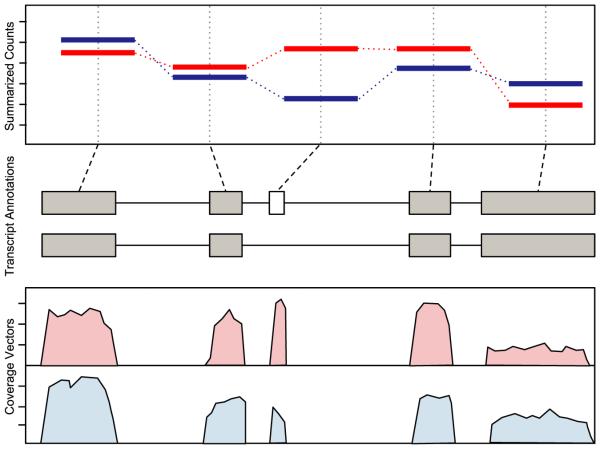
There are three primary types of data in genomics: sequence vectors, annotated ranges and feature-by-sample matrices of summary statistics (Figure 1). Biological sequences are represented as strings of characters from a restricted alphabet. For example, a DNA sequence consists of the letters A, C, G and T, each referring to a particular type of nucleotide. A genome consists of a set of DNA sequences, one for each chromosome. We generalize the concept of sequence and define the term sequence vector to mean either a sequence or a vector that runs parallel to a sequence. The latter may be some curated or computed value, such as the cross-species conservation or coverage from a sequencing experiment. The coverage is a common summary that represents the number of features overlapping each position in the reference sequence.

Fig. 1.

Cartoon visualization of all three types of genomic data: genome-length vectors, ranged, features and summaries (from bottom to top). Data from two samples are compared (red vs. blue). The bottom plot displays the coverage, a genome-length vector. The exon ranges are shown in the middle. The top plot presents summaries, the per-exon read counts.

As we learn more about a genome, we annotate genomic ranges with information like gene structures and regulatory binding sites. The alignment of sequences to a reference genome is another type of range-based annotation.

To compare data across samples, we often summarize experimental annotations over a set of reference features to yield a feature-by-sample matrix. For example, we might count read alignments overlapping a common set of genes across a number of samples. Larger matrices often arise in genetics, where thousands of samples are compared over millions of SNPs, positions that are known to vary within a population. In every case, the summaries are tied to a genomic range.

To analyze the results of an experiment, we need to integrate data of different types. For example, we might have alignments for a ChIP-seq experiment, where the sequences have been enriched for binding to a particular transcription factor. A typical analysis involves checking coincidence with annotated binding sites for that transcription factor, as well as looking for correlation between gene expression and binding signal upstream of the gene. The gene expression values might be drawn from a gene by a sample matrix summarized from an RNA-seq experiment. The genomic range is the common thread that integrates all three types of data. The sequence, that is, the genome, acts as the scaffold, and ranges coordinate the annotations and summarized features by locating them on the same sequence.

The R language [13] is widely applied to problems in statistics and data analysis, including the analysis of genomic data [8], as evidenced by the large number of available software packages providing features ranging from data manipulation to machine learning. R provides high-level programming abstractions that make it accessible to statisticians and bioinformatics professionals who are not software engineers per se. One aspect of R that is particularly useful is its “copy on write” memory semantics, which insulates the user from the details of reference-based memory management. The fundamental R data structure is the atomic vector, which is both convenient and efficient for moderately sized data. An atomic vector is homogeneous in data type and so easily stored in one contiguous block of memory. Many vector operations are implemented in native (C) code, which avoids invoking the R interpreter as it iterates over vector elements. In a typical multivariate data set, there is heterogeneity in data type across the columns and homogeneity along a column, so vectors are naturally suited for column-oriented data storage, as in the basic data.frame. Vectorized computations can usually be expressed with simpler and more concise code compared to explicit iteration. The strengths of R are also its weaknesses: the R API encourages users to store entire data sets in memory as vectors. These vectors are implicitly and silently copied to achieve copy-on-write semantics, contributing to high memory usage and poor performance.

There are general strategies for handling large genomic data that are well suited to R programs. Sometimes the analyst is only interested in one aspect of the data, such as that overlapping a single gene. In such cases, restricting the data to that subset is a valid and effective means of data reduction. However, once our interests extend beyond a single region or the region becomes too large, resource constraints dictate that we cannot load the entire data set into memory at once, and we need to iterate over the data to reduce them to a set of interpretable summaries.

Iteration lends itself to parallelism, that is, computing on multiple parts of the same problem simultaneously. Thus, in addition to meeting memory constraints, iteration lets us leverage additional processing resources to reduce overall computation time. Investing in additional hardware is often more economical than investment in software optimization. This is particularly relevant in scientific computing, where we are faced with a diverse, rapidly evolving set of unsolved problems, each requiring specialized software. The costs of investment in general purpose hardware are amortized over each problem, rather than paid each time for software optimization. This also relates to maintainability: optimization typically comes at a cost of increased code complexity. Many types of summary and filter operations are cheap to implement in parallel because the data partitions can be processed independently. We call this type of operation embarrassingly parallel. For example, the counting of reads overlapping a gene does not depend on the counting for a different gene.

Given the complexity and scope of the data, analysts often rely on visual tools that display summaries and restricted views to communicate information at different scales and level of detail, from the whole genome to single nucleotide resolution. Plot interactivity is always a useful feature when exploring data, and this is particularly true with big data. The view is always restricted in terms of its region and detail level, so, in order to gain a broader and deeper understanding of the data, the viewer will need to adjust the view, either by panning to a different region, zooming to see more details or adjusting the parameters of the summary step. The size of the genome and the range of scales make it infeasible to pre-render every possible view. Thus, the views need to be generated dynamically, in lazy reaction to the user. Performance is an important factor in interpretability: slow transitions distract the viewer and obfuscate relationships between views. Dynamic generation requires fast underlying computations to load, filter and summarize the data, and fast rendering to display the processed data on the screen.

This paper describes strategies to surmount computational and visualization challenges in the analysis of large genomic data and how they have been implemented in the R programming language by a number of packages from the Bioconductor project [5]. We will demonstrate their application to a real data set: the whole-genome sequencing of the HapMap cell line NA12878, the daughter in the CEU trio. The GATK project genotyped the sample according to their best practices and included the calls in their resource bundle, along with the alignments for chr20, one of the shortest chromosomes. Realistically, one would analyze the data for the entire genome, but the chr20 subset is still too large to be processed on a commodity laptop and thus is sufficient for our purposes.

2. LIMITING RESOURCE CONSUMPTION

Our ultimate goal is to process and summarize a large data set in its entirety, and iteration enables this by limiting the resource commitment at a given point in time. Limiting resource consumption generalizes beyond iteration and is a fundamental technique for computing with big data. In many cases, it may render iteration unnecessary. Two effective approaches for being frugal with data are restriction and compression. Restriction means controlling which data are loaded and lets us avoid wasting resources on irrelevant or excessive data. Compression helps by representing the same data with fewer resources.

2.1 Restricting Queries

Restriction is appropriate when the question of interest requires only a fraction of the available data. It is applicable in different ways to sequence vectors, range-based annotations and feature-by-sample matrices. We can restrict data along two dimensions: row/record-wise and/or column/attribute-wise, with genomic overlap being an important row filter. Sequences and genomic vectors are relatively simple structures that are often restricted by range, that is, extraction of a contiguous subsequence of per-position values. Row-wise restriction is useful when working with large sets of experimentally generated short sequences. The sequence aligner generates alignments as annotations on a reference sequence, and these alignments have many attributes, such as genomic position, score, gaps, sequence and sequence quality. Restriction can exclude the irrelevant attributes. Analysts often slice large matrices, such as those consisting of SNP calls, by both row (SNP) and column (individual).

A special mode of restriction is to randomly generate a selection of records. Down-sampling can address many questions, especially during quality assessment and data exploration. For example, short reads are initially summarized in FASTQ files containing a plain text representation of base calls and corresponding quality scores. Basic statistics of quality assessment such as the nucleotide count as a function of sequencing cycle or overall GC content are very well characterized by random samples of a million reads, which might be 1% of the data. This sample fits easily in memory. Computations on this size of data are very nimble, enabling interactive exploration on commodity computers. An essential requirement is that the data represent a random sample.

The ShortRead package is designed for the QA and exploratory analysis of the output from high-througput sequencing instruments. It defines the Fastq Sampler object, which draws random samples from FASTQ files. The sequence reads in our data set have been extracted into a FASTQ file from the publicly available alignments. We wish to check a few quality statistics before proceeding. We begin by loading a random sample of one million reads from the file:

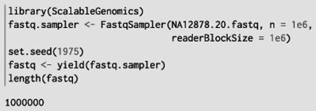
With the sequences loaded, we can compute some QA statistics, like the overall base call tally:

In a complete workflow, we would generate an HTML QA report via the report function.

An example of a situation where random sampling does not work is when prototyping a statistical method that depends on a significant amount of data to achieve reasonable power. Variant calling is a specific example: restricting the number of reads would lead to less coverage, less power and less meaningful results. Instead, we need to restrict the analysis to a particular region and include all of the reads falling within it.

To optimize range-based queries, we often sort and index our data structures by genomic coordinates. We should consider indexing an investment because an index is generally expensive to generate but cheap to query. The justification is that we will issue a sufficient number of queries to outweigh the initial generation cost. Three primary file formats follow this pattern: BAM, Tabix and BigWig [7, 10]. Each format is best suited for a particular type of data. The BAM format is specially designed for sequence alignments and stores the complex alignment structure, as well as the aligned sequence. Tabix is meant for indexing general range-based annotations stored in tabular text files, such as BED and GFF. Finally, BigWig is optimized for storing genome-length vectors, such as the coverage from a sequencing experiment. BAM and Tabix compress the primary data with block-wise gzip compression and save the index as a separate file. BigWig files are similarly compressed but are self-contained.

The Rsamtools package is an interface between R and the samtools library, which implements access to BAM, Tabix and other binary file formats. Rsamtools enables restriction of BAM queries through the Scan Bam Param object. This object can be used as an argument to all BAM input functions, and enables restriction to particular fields of the BAM file, to specific genomic regions of interest and to properties of the aligned reads (e.g., restricting input to paired-end alignments that form proper pairs).

One common scenario in high-throughput sequencing is the calculation of statistics such as coverage (the number of short sequence reads overlapping each nucleotide in the genome). The data required for this calculation usually come from very large BAM files containing alignment coordinates (including the alignment “cigar”), sequences and quality scores for tens of millions of short reads. Only the smallest element of these data, the alignment coordinates, is required for calculation of coverage. By restricting input to alignment coordinates, we transform the computational task from one of complicated memory management of large data to simple vectorized operations on in-memory objects.

We can directly implement a coverage estimation by specifying a Scan Bam Param object that restricts to the alignment information. The underlying coverage calculation is implemented by the IRanges package, which sits at the core of the Bioconductor infrastructure and provides fundamental algorithms and data structures for manipulating and annotating ranges. It is extended by GenomicRanges to add conveniences for manipulating ranges on the genome:

This is only an estimate, however, because we have ignored the complex structure of the alignments, for example, the insertions and deletions. Rsamtools provides a convenience function for the more accurate calculation:

2.2 Compressing Genomic Vectors

Some vectors, in particular, the coverage, have long stretches of repeated values, often zeroes. An efficient compression scheme for such cases is run-length encoding. Each run of repeated values is reduced to two values: the length of the run and the repeated value. This scheme saves space and also reduces computation time by reducing computation size. For example, the vector 0, 0, 0, 1, 1, 5, 5, 5 would have run-values 0, 1, 5 and run-lengths 3, 2, 3. The data have been reduced from a size of 8 to a size of 6 (3 values plus 3 lengths). The IRanges Rle class is a run-length encoded vector that supports the full R vector API on top of the compressed representation. Operations on an Rle gain efficiency by taking advantage of the compression. For example, the sum method computes a sum of the run values, using the run lengths as weights. Thus, the time complexity is on the order of the number of runs, rather than the length of the vector.

The cov object we generated in the previous section is a list of Rle objects, one per chromosome.

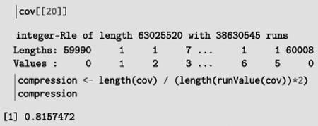
For this whole-genome sequencing, the data are quite dense and complex, so the compression actually decreases efficiency. However, in the course of analysis we often end up with sparser data and thus better compression ratios. In this analysis, we are concerned about regions with extremely high coverage: these are often due to alignment artifacts.

Calculating the sum is then more efficient than with conventional vectors:

Sometimes we are interested in the values of a genomic vector that fall within a set of genomic features. Examples include the coverage values within a set of called ChIP-seq peaks or the conservation scores for a set of motif hits. We could extract the subvectors of interest into a list. However, large lists bring undesirable overhead, and the data would no longer be easily indexed by genomic position. Instead, we combine the original vector with the ranges of interest. In IRanges, this is called a Views object. There is an Rle Views object for defining views on top of an Rle.

To demonstrate, we slice our original coverage vector by our high coverage cutoff to yield the regions of high coverage, overlaid on the coverage itself, as an Rle Views object:

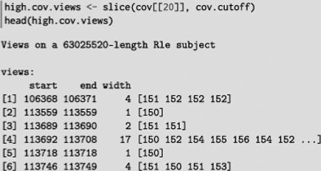
This lets us efficiently calculate the average coverage in each region:

The Biostrings package [12] provides X String Views for views on top of DNA, RNA and amino acid sequences. X String is a reference, rather than a value as is typical in R, so we can create multiple X String Views objects without copying the underlying data. This is an application of the fly-weight design pattern: multiple objects decorate the same primary data structure, which is stored only once in memory.

We can apply X String Views for tabulating the nucleotides underlying the high coverage regions. First, we need to load the sequence for chr20, via the BSgenome package and the addon package for human:

While the human genome consists of billions of bases, our genome object is tiny. This is an example of lazy loading: chromosomes are loaded, and cached, as requested. In our case, we restrict to chr20 and form the X String Views.

We verify that the cached sequence occupies the same memory as the subject of the views:

Finally, we calculate and compare the nucleotide frequencies:

We notice that the high coverage regions are A/T-rich, which is characteristic of low complexity regions.

2.3 Compressing Lists

The high coverage regions in our data may be associated with the presence of repetitive elements that confuse the aligner. We obtain the repeat annotations from the UCSC genome browser with the rtracklayer package, which, in addition to a browser interface, handles input and output for various annotation file formats, including BigWig. Our query for the repeats is restricted to chr20, which saves download time. We subset to the simple and low complexity repeats, which are the most likely to be problematic:

Our goal is to calculate the percent of each high coverage region covered by a repeat. First, we split the repeats according to overlap with a high coverage region:

The repeats.split object is not an ordinary list. Long lists are expensive to construct, store and process. Creating a new vector for each group requires time, and there is storage overhead for each vector. Furthermore, data compression is less efficient when the data are split across objects. Depending on the implementation of the list elements, these costs can be significant. This is particularly true of the S4 object system in R [2]. Another detriment to R lists is that list elements can be of mixed type. Thus, there are few native routines for computing on lists. For example, the R sum function efficiently sums the elements of a homogeneous numeric vector, but there is no support for calling sum to calculate the sum of each numeric vector in a list. Even if such routines did exist for native data types, there are custom data types, such as ranges, and we aim to facilitate grouping of any data that we can model as a vector.

While the R sum function is incapable of computing group sums, there is an oddly named function called rowsum that will efficiently compute them, given a numeric vector and a grouping factor. This hints that a more efficient approach to grouping may be to store the original vector along with a partitioning. The IRanges R package includes a Compressed List framework that follows this strategy. A Compressed List consists of the data vector, sorted by group, and a vector of indexes where each group ends in the data vector (see Figure 2). IRanges provides Compressed List implementations for native atomic vectors and other data types in the IRanges infrastructure, and the framework is extensible to new data types. A Compressed List is homogeneous, so it is natural to define methods on subclasses to perform operations particular to a type of data. For example, there is a sum method for the Numeric List class that delegates internally to rowsum. This approach bears similarity to storing data by columns: we improve storage efficiency by storing fewer objects, and we maintain the data in its most readily computable form. It is also an application of lazy computing, where we delay the partitioning of the data until a computation requires it. We are then in position to optimize the partitioning according to the specific requirements of the operation.

Fig. 2.

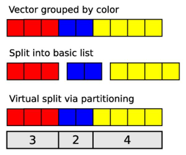
Grouping via partitioning vs. splitting into multiple objects. Top: the input vector, with elements belonging to three different groups: red, blue and yellow. Middle: typical splitting of vector into three vectors, one per group. This brings the overhead of multiple objects. Bottom: the data are virtually split by a partitioning, encoded by the number of elements in each group (the vector is assumed to be sorted by group).

Since repeats.list is a Compressed List, we can take advantage of these optimizations:

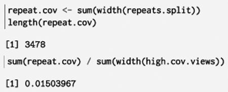
This value can be compared to the percent of chr20 covered:

Instead of a Compressed List, we could have solved this problem using coverage and Rle Views.

The downside of compression is that there is overhead to explicit iteration because we need to extract a new vector with each step. The Biostrings package has explored a solution. We can convert our X String Views object chr20.views to a DNA-String Set that contains one DNA String for each view window. The data for each DNA String has never been copied from the original chr20 sequence, and any operations on a DNA String operate directly on the shared data. While this solution may seem obvious, it relies heavily on native code and is far from the typical behavior of R data structures:

The nascent XVector package aims to do the same for other R data types, such as integer, double and logical values.

3. ITERATING

3.1 Splitting Data

Iterative summarization of data may be modeled as three separate steps: split, apply and combine [15]. The split step is typically the only one that depends on the size of the input data. The apply step operates on data of restricted size, and it should reduce the data to a scale that facilitates combination. Thus, the most challenging step is the first: splitting the data into chunks small enough to meet resource constraints.

Two modes of splitting are particularly applicable to genomic data: sequential chunking and genomic partitioning. Sequential chunking is a popular and general technique that simply loads records in fixed-count chunks, according to the order in which they are stored. Genomic partitioning iterates over a disjoint set of ranges that cover the genome. Typical partitioning schemes include one range per chromosome and sub-chromosomal ranges of some uniform size. Efficient range-based iteration, whether over a partitioning or list of interesting regions, depends on data structures, file formats and algorithms that are optimized for range-based queries.

Under the assumption that repeat regions are leading to anomalous alignments, we aim to filter from our BAM file any alignments overlapping a repeat. As we will be performing many overlap queries against the repeat data set, it is worth indexing it for faster queries. The algorithms for accessing BAM, Tabix and BigWig files are designed for genome browsers and have not been optimized for processing multiple queries in a batch. Each query results in a new search. This is unnecessarily wasteful, at least when the query ranges are sorted, as is often the case. We could improve the algorithm by detecting whether the next range is in the same bin and, if so, continuing the search from the current position. The IRanges package identifies interval trees [3] as an appropriate and well-understood data structure for range-based queries, and implements these using a combination of existing C libraries [6] and new C source code. The query is sorted, and every new search begins at the current node, rather than at the root. We build a GIntervalTree for the repeats:

The G Interval Tree from GenomicRanges enables the same optimization when data are aligned to multiple chromosomes.

To configure streaming, we specify a yield Size when constructing the object representing our BAM file. We will filter at the individual read level, but it should be noted that for paired-end data Rsamtools supports streaming by read pair, such that members of the same pair are guaranteed to be in the same chunk. Since BAM files are typically sorted by position, not pair, this is a significant benefit:

To filter the BAM, we first need to define a filter rule that excludes reads that overlap a repeat. The low-level Rsamtools interface provides the read data as a Data Frame, which we convert into a G Alignments object from the GenomicAlignments package, which provides data structures and utilities for analyzing read alignments:

Since we are writing a new BAM file, this is iteration with a side effect rather than a reduction.

To demonstrate reduction, we will calculate the coverage in an iterative fashion, which ends up identical to our original calculation:

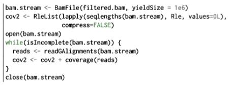
Choosing an appropriate yield size for each iteration is important. There is overhead to each iteration, mostly due to I/O and memory allocation, as well as the R evaluator. Thus, one strategy is to increase the size of each iteration (and reduce the number of iterations) until the data fit comfortably in memory. It is relatively easy to estimate a workable yield size from the consumption of processing a single chunk. The gc function exposes the maximum amount of memory consumed by R between resets:

The memory usage started at about 500 MB and peaked at about 1200 MB, so the iteration consumed up to 700 MB. With 8 GB of ram, we might be able to process up to 10 million reads at once, assuming linear scaling.

As an alternative to streaming over chunks, we can iterate over a partitioning of the genome or other domain. Genomic partitioning can be preferable to streaming when we are only interested in certain regions. The tile Genome function is a convenience for generating a set of ranges that partition a genome. We rely on it to reimplement the coverage iterative calculation with a partitioning:

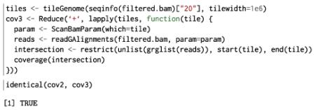
A caveat with partitioning is that since many query algorithms return ranges with any overlap of the query, care must be taken to intersect the results with each partition, so that reads are not double counted, for example.

By computing the coverage, we have summarized the data. Computing summaries is often time consuming, but since the summaries are smaller than the original data, it is feasible to store them for later use. Caching the results of computations is an optimization technique known as memoization. An analysis rarely follows a linear path. By caching the data at each stage of the analysis, as we proceed from the raw data to a feature-level summary, often with multiple rounds of feature annotation, we can avoid redundant computation when we inevitably backtrack and form branches. This is an application of incremental computing. We export our coverage as a BigWig file, for later use:

3.2 Iterating in Parallel

There are two basic modes of parallelism: data-level and task-level. Embarrassingly parallel problems illustrate data parallelism. Work flows might less frequently involve task parallelism, where different tasks are applied to the same data chunk. These are generally more challenging to implement, especially with R, which does not offer any special support for concurrency. The Streamer package has explored this direction.

Multicore and cluster computing are similar in that they are modular, and scaling algorithms to use multiple cores or multiple nodes can involve conceptually similar steps, but there are some critical differences. Multiple cores in the same system share the same memory, as well as other resources. Shared memory configurations offer fast inter-thread data transfer and communication. However, the shared resources can quickly become exhausted and present a bottleneck. Computing on a cluster involves significant additional expertise to access and manage cluster resources that are shared between multiple users and governed by a scheduler. Interacting with a scheduler introduces an extra step into a workflow. We place jobs in a queue, and the jobs are executed asynchronously. Another complication is that we need to share the data between every computer. A naive but often sufficient method is to store the data in a central location on a network file system and to distribute the data via the network. The network overhead implied by this approach may penalize performance.

When the ratio of communication to computation time is large, communication dominates the overall calculation. The main strategies for addressing this are to (a) ensure each task represents a significant amount of work and (b) identify points where data sizes of inputs (e.g., file names) and outputs (e.g., vector of counts across regions of interest) are small. Data partitioning is usually conveyed to workers indirectly, for example, via specification of the range of data to be processed, rather than inputting and explicitly partitioning data. This approach reduces the communication costs between the serial and parallel portions of the computation and avoids loading the entire data set into memory.

The R packages foreach [14], parallel (distributed with R [13]), pbdR [11] and BatchJobs [1] provide abstractions and implementations for executing tasks in parallel and support both the shared memory and cluster configurations. BatchJobs and pbdR are primarily designed for asynchronous execution, where jobs are submitted to a scheduling system, and the user issues commands to query for job status and collect results upon completion. The other two, foreach and parallel, follow a synchronous model conducive to interactive use.

Different use cases and hardware configurations benefit from different parallelization strategies. An analyst might apply multiple strategies in the course of an analysis. This has motivated the development of an abstraction oriented toward genomics workflows. The BiocParallel package defines this abstraction and implements it on top of BatchJobs, parallel and foreach to support the most common configurations. An important feature of BiocParallel is that it encapsulates the parallelization strategy in a parameter object that can be passed down the stack to infrastructure routines that implement the iteration. Thus, for common use cases the user can take advantage of parallelism by solely indicating the appropriate implementation. Iteration is carried out in a functional manner, so the API mirrors the *apply functions in base R: bplapply, bpmapply, etc.

To illustrate use of parallel iteration, we diagnose the GATK genotype calls introduced earlier. One approach is to generate our own set of nucleotide tallies, perform some simple filtering to yield a set of variant calls, and compare our findings to those from GATK. The set of nucleotide tallies is a more detailed form of the coverage that consists of the count of each nucleotide at each position, as well as some other per-position statistics. Tallies are useful for detecting genetic variants through comparison to a reference sequence.

The VariantTools package provides a facility for summarizing the nucleotide counts from a BAM file over a given range. We can iterate over the tiling in parallel using the bplapply function. The BPPARAM argument specifies the parallel implementation. Multicore Param is appropriate for a multicore workstation, whereas we might use Batch Jobs Param for scheduling each iteration as a job on a cluster:

The above is an example of explicit iteration. Thanks to the encapsulation and abstraction afforded by Bioc Parallel Param, the pileup Variants function supports parallel iteration directly, so the implementation becomes much simpler:

This is an example of an embarrassingly parallel solution: each iteration is a simple counting exercise and is independent of the others. An example of a nonembarrassingly parallel algorithm is our demonstration of BAM filtering: each iteration has the side effect of writing to the same file on disk. The increased complexity of coordinating the I/O across jobs undermines the value of parallelism in that case.

4. SCALING GENOMIC GRAPHICS

4.1 Managing Graphical Resources

Graphics software is special in that it performs two roles: distilling information from the data and visually communicating that information to the user. The first role is similar to any data processing pipeline; the unique aspect is the communication. The communication bandwidth of a plot is limited by the size and resolution of the display device and the perceptive capabilities of the user. These limitations become particularly acute in genomics, where it would be virtually impossible to communicate the details of a billion alignments along a genome of 3 billion nucleotides.

When considering how best to manage graphical resources, we recall the general technique of restriction. Restriction has obvious applicability to genomic graphics: we can balance the size of the view and the level of detail. As we increase the size of the view, we must decrease the level of detail and vice versa. This means only so much information can be communicated in a single plot, so the user needs to view many plots in order to comprehend the data. It would be infeasible to iteratively generate every possible plot, so we need to lazily generate plots in response to user interaction. For example, the typical genome browser supports panning and zooming about the genome, displaying data at different levels of detail, depending on the size of the genomic region.

4.2 Displaying Summaries Efficiently

When plotting data along a restricted range, graphics software can rely on the support for range-based queries presented previously. Controlling the level of detail is more challenging because it relies on summaries. As the viewed region can be as large as the genome, generating summaries is often computationally intensive and introduces undesirable latency to plot updates. One solution to this problem is caching summaries at different levels of detail. Global summaries will be regularly accessed and expensive to compute, and thus are worth caching, whereas the detailed data exposed upon drill-down can be computed lazily. This strategy is supported by the BigWig format. In addition to storing a full genomic vector, BigWig files also contain summary vectors, computed over a range of resolutions, according to the following statistics: mean, min, max and standard deviation. Plotting the aggregate coverage is a shortcut that avoids pointless rendering of data that is beyond the display resolution and the perceptive abilities of the viewer:

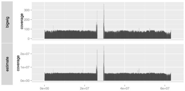
A good summary will guide the user to the most interesting parts of the data. Genomic data are typically sparsely distributed along the genome, due to the nonuniform distribution of genes and experimental protocols that enrich for regions of interest. Coverage is a particularly useful summary, as it helps guide the viewer to the regions with the most data. The following gets the average coverage for 800 windows (perhaps appropriate for an 800 pixel plot). The result is shown in the top panel of Figure 3:

Fig. 3.

The results of two coverage calculations over chr20. Top: the calculation based on cached values in the BigWig file. Bottom: the estimated coverage from the BAM index file.

In cases where a BigWig file or other cached summary is unavailable, we can rely on a heuristic that estimates the coverage from the index of a BAM or Tabix file. The index stores offsets into the BAM for efficient rangebased queries. Instead of accessing the index to resolve queries, we calculate the difference in the file offsets for each range and derive a relative coverage estimate at a coarse level of resolution. In practice, this reduces the required time to compute the coverage from many minutes to a few seconds. When the plot resolution exceeds the resolution of the index, we again rely on the index to query the BAM file for the reads that fall within the relatively small region and compute the coverage directly. A heuristic seems acceptable in this case, because improved accuracy is immediately accessible by zooming. This is in contrast to pure statistical computations, where crude estimates are less appreciated, even in the exploratory context, since resolution is not so readily forthcoming.

The estimate Coverage function from the biovizBase package [17] estimates the coverage from the BAM index file. The bottom panel of Figure 3 shows the output of estimate Coverage for the example data set and allows for comparison with the more exact calculation derived from the BigWig file. The two results are quite similar and both required only a few seconds to compute on a commodity laptop.

4.3 Generating Plots Dynamically

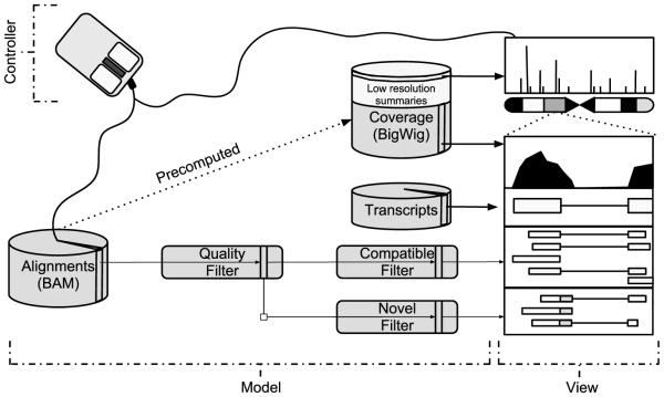
The design of interactive graphics software typically follows the model–view–controller pattern (see Figure 4). The view renders data retrieved from the data model, and the controller is the interface through which the user manipulates the view and data model. The data model abstracts the underlying data source, which might be memory, disk or a dynamic computation. The abstraction supports the implementation of complex optimizations without exposing any of the complexity to client code. Data is communicated to the user through the view, and user input is received through the controller. A complex application will consist of multiple interactive views, linked through a common data model, itself composed of multiple modules, chained together as stages in a pipeline. The viewer, plots and pipeline stages are interlinked to form a network.

Fig. 4.

An application of the model–view–controller pattern and pre-computed summaries to genomic visualization. Coverage is displayed at two levels of resolution (whole chromosome and the current zoom) after efficient extraction from the multi-resolution BigWig file. The BAM file holding the read alignments is abstracted by a multi-stage data model, consisting of the BAM source, a dynamic read quality filter and two filters that effectively split the alignments according to compatibility with the known transcript annotations. The view contains several coordinately-zoomed plots, as well as an ideogram and coverage overview. Each plot obtains its data from one of the data model components. The controller might adjust the data model filter settings and the current zoom in response to user commands.

A simple data model abstracts access to the primary data, such as an in-memory GRanges object of transcript annotations or a BAM file on disk. We can extend the simple model to one that dynamically computes on data as they are requested by the application. This is an example of lazy computing. Each operation is encapsulated into a data model that proxies an underlying model. The proxy models form a chain, leading from the raw data to the processed data that are ready for plotting [16]. Dynamic computation avoids unnecessarily processing the entire genome when the user is only interested in a few small regions, especially when the parameters of the transformations frequently change during the session. The data may be cached as they are computed, and the pipeline might also anticipate future requests; for example, it might prepare the data on either side of the currently viewed region, in anticipation of scrolling. Caching and prediction are examples of complex optimizations that are hidden by the data model. The plumbr R package [9] provides a proxy model framework for implementing these types of ideas behind the data frame API.

We have been experimenting with extending these approaches to genomic data. The biovizBase package implements a graphics-friendly API for restricted queries to Bioconductor-supported data sources. The ggbio package builds on biovizBase to support genomic plot objects that are regenerated as the user adjusts the viewport.

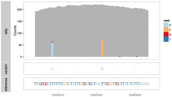
To diagnose the GATK genotype calls, we combine the reference sequence, nucleotide pileup and the genotype calls. The result is shown in Figure 5. The ggbio package produced the plot by relying on restricted query support in biovizBase. We have already introduced the extraction of genomic sequence and the calculation of nucleotide pileups. The genotypes were drawn by the VariantAnnotation package from a Variant Call Format (VCF, [4]) file with a range-based index provided by Tabix.

Fig. 5.

Example plot for diagnosing genotype calls, consisting of the nucleotide tallies, genotype calls and reference sequence, from top to bottom. The plot is dynamically generated for the selected region of interest, without processing the entire genome. The viewer might check to see if the tallies support the called genotypes. In this case, the data are consistent.

To generate the plot, we first select the region of interest:

Next, we construct the plot object and render it:

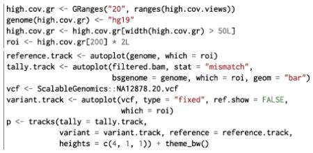
Since the plot object is a logical representation of the plot, that is, it references the original data, we can adjust various aspects of it and generate a new rendering. In particular, we can change the currently viewed region, and the data for the new region are processed dynamically to generate the new plot. In this example, we zoom out to a larger region around the first region:

Current work is focused on the MutableRanges package, which generalizes and formalizes the designs in biovizBase. It defines dynamic versions of the GenomicRanges data structures, for example, there is a DynamicGRanges that implements the GRanges API on top of a BAM file. Only the requested regions are loaded, and they are optionally cached for future queries. A ProxyGRanges performs dynamic computations based on another GRanges. This will enable a new generation of interactive genomic visualization tools in R. An early adopter is epivizr, the R interface to the web-based epiviz, a web-based genome browser with support for general interactive graphics, including scatterplots and histograms.

5. CONCLUSION

We have introduced software and techniques for analyzing and plotting big genomic data. The Bioconductor project distributes the software as a number of different R packages, including Rsamtools, IRanges, GenomicRanges, GenomicAlignments, Biostrings, rtracklayer, biovizBase and BiocParallel. The software enables the analyst to conserve computational resources, iteratively generate summaries and visualize data at arbitrary levels of detail. These advances have helped to ensure that R and Bioconductor remain relevant in the age of high-throughput sequencing. We plan to continue in this direction by designing and implementing abstractions that enable user code to be agnostic to the mode of data storage, whether it be memory, files or databases. This will bring much needed agility to resource allocation and will enable the user to be more resourceful, without the burden of increased complexity.

REFERENCES

- [1].Bischl B, Lang M, Mersmann O, Rahnenfuehrer J, Weihs C. Technical Report 1. TU Dortmund; 2011. Computing on high performance clusters with R: Packages BatchJobs and BatchExperiments. [Google Scholar]
- [2].Chambers JM. Software for Data Analysis: Programming with R. Springer; New York: 2008. [Google Scholar]
- [3].Cormen TH, Leiserson CE, Rivest RL, Stein C. In: Introduction to Algorithms. 2nd. McGraw-Hill, editor. Boston, MA: 2001. MR1848805. [Google Scholar]
- [4].Danecek P, Auton A, Abecasis G, Albers CA, Banks E, DePristo MA, Handsaker RE, Lunter G, Marth GT, Sherry ST, McVean G, Durbin R, 1000 Genomes Project Analysis Group The variant call format and VCFtools. Bioinformatics. 2011;27:2156–2158. doi: 10.1093/bioinformatics/btr330. [DOI] [PMC free article] [PubMed] [Google Scholar]
- [5].Gentleman RC, Carey VJ, Bates DM, others Bioconductor: Open software development for computational biology and bioinformatics. Genome Biol. 2004;5:R80. doi: 10.1186/gb-2004-5-10-r80. [DOI] [PMC free article] [PubMed] [Google Scholar]
- [6].Kent WJ, Sugnet CW, Furey TS, Roskin KM, Pringle TH, Zahler AM, Haussler D. The human genome browser at UCSC. Genome Res. 2002;12:996–1006. doi: 10.1101/gr.229102. [DOI] [PMC free article] [PubMed] [Google Scholar]
- [7].Kent WJ, Zweig AS, Barber G, Hinrichs AS, Karolchik D. BigWig and BigBed: Enabling browsing of large distributed datasets. Bioinformatics. 2010;26:2204–2207. doi: 10.1093/bioinformatics/btq351. [DOI] [PMC free article] [PubMed] [Google Scholar]
- [8].Lawrence M, Huber W, Pagès H, Aboyoun P, Carlson M, Gentleman R, Morgan M, Carey V. Software for computing and annotating genomic ranges. PLoS Computational Biology. 2013;9:e1003118. doi: 10.1371/journal.pcbi.1003118. [DOI] [PMC free article] [PubMed] [Google Scholar]
- [9].Lawrence M, Wickham H. plumbr: Mutable and dynamic data models. R package version 0.6.6. 2012 [Google Scholar]
- [10].Li H, Handsaker B, Wysoker A, Fennell T, Ruan J, Homer N, Marth G, Abecasis G, Durbin R, 1000 Genome Project Data Processing Subgroup The Sequence Alignment/Map format and SAMtools. Bioinformatics. 2009;25:2078–2079. doi: 10.1093/bioinformatics/btp352. [DOI] [PMC free article] [PubMed] [Google Scholar]
- [11].Ostrouchov G, Chen W-C, Schmidt D, Patel P. Programming with big data in R. 2012 Available at http://r-pbd.org/
- [12].Pagès H, Aboyoun P, Gentleman R, DebRoy S. Biostrings: String objects representing biological sequences, and matching algorithms. R package version 2.25.6. 2013 [Google Scholar]
- [13].R Development Core Team . R: A Language and Environment for Statistical Computing. R Foundation for Statistical Computing; Vienna, Austria: 2010. [Google Scholar]
- [14].Revolution Analytics. Weston S. foreach: Foreach looping construct for R. R package version 1.4.1. 2013 [Google Scholar]
- [15].Wickham H. The split-apply-combine strategy for data analysis. Journal of Statistical Software. 2011;40:1–29. [Google Scholar]
- [16].Wickham H, Lawrence M, Cook D, Buja A, Hofmann H, Swayne DF. The plumbing of interactive graphics. Comput. Statist. 2009;24:207–215. MR2506079. [Google Scholar]
- [17].Yin T, Lawrence M, Cook D. biovizBase: Basic graphic utilities for visualization of genomic data. R package version 1.9.1. 2013 [Google Scholar]