Determination of the ribosome structure to a resolution of 2.5 Å by single‐particle cryo‐EM

Abstract

With the advance of new instruments and algorithms, and the accumulation of experience over decades, single‐particle cryo‐EM has become a pivotal part of structural biology. Recently, we determined the structure of a eukaryotic ribosome at 2.5 Å for the large subunit. The ribosome was derived from Trypanosoma cruzi, the protozoan pathogen of Chagas disease. The high‐resolution density map allowed us to discern a large number of unprecedented details including rRNA modifications, water molecules, and ions such as Mg²⁺ and Zn²⁺. In this paper, we focus on the procedures for data collection, image processing, and modeling, with particular emphasis on factors that contributed to the attainment of high resolution. The methods described here are readily applicable to other macromolecules for high‐resolution reconstruction by single‐particle cryo‐EM.

Introduction

In the past three years, single‐particle cryo‐EM, a technique developed in the last three decades, has revolutionized structural biology and has gained popularity in academic and, increasingly, industrial research. The revolution is manifested in three aspects: the high resolution, comparable with that obtained in X‐ray crystallography; the capacity to determine multiple structures co‐existing in the same sample; and the proven capability of solving small membrane proteins and large supra‐macromolecular complexes, which are both difficult to solve by X‐ray crystallography.

With traditional recording devices, the best resolution for asymmetric molecules such as ribosomes was not better than 5 Å.1, 2 It has now moved into the range of 2–3 Å, permitting de novo atomic modeling.3, 4, 5, 6 Improvements in the data quality of cryo‐EM have been provided primarily by advances in instrumentation. First of all, the direct electron detector device (DDD) dramatically improves the Detection Quantum Efficiency (DQE) and allows fractionating the electron dose of each micrograph.7 In this way, radiation damage can be reduced a posteriori by selecting a subset of frames, and the beam‐induced movement of the sample can be compensated by correcting the displacements among the frames. In addition to the introduction of direct electron detectors, spherical aberration (Cs) correction,5 energy filtration8 and the addition of a phase plate are all measures that have the potential to improve image quality and resolution.9

The ribosome has served as a benchmark sample for decades in the development of single‐particle cryo‐EM.10 Sub‐3 Å resolution of ribosomes, in the range of 2.5–2.9 Å, has now been achieved by four groups.3, 4, 5, 6 Our own 2.5‐Å cryo‐EM reconstruction6 is of the ribosome extracted from Trypanosome cruzi, a protozoan pathogen causing Chagas disease in humans. This ribosome, as those from other trypanosomatids, possesses a 28S rRNA composed of six fragments. The high‐resolution structure not only reveals the precise interactions stabilizing the RNA but also provides insights that may allow the design of safe trypanosome‐specific drugs. Our work makes judicious use of recent advances in cryo‐EM methodology including instrumentation, image acquisition, and image processing algorithms, modeling tools and computing resources. Achievement of the highest resolution, beyond 3 Å, requires bottlenecks to be eliminated that are not present at lower resolution. The following sections will describe each of these steps and discuss the rationales for the choices of conditions and parameters in optimizing the results.

Data Collection

In our experiments for the T. cruzi project, we made use of the FEI Falcon 2 camera installed on the Titan Krios microscope (FEI, Eindhoven) with a Cs corrector and EPU software for imaging our sample, in preference to an FEI Tecani F30 Polara microscope equipped with a K2 Summit (Gatan, Pleasanton) available in house. The whole dataset was collected in a single pass of five consecutive days, yielding about 11,000 micrographs with a speed of about 100 micrographs per hour. Thus, high throughput of imaging allowed collection of a big dataset with sufficient numbers of particles for high‐resolution reconstruction, even covering different states of the ribosome.

The electron microscope

For high‐resolution single‐particle cryo‐EM, transmission electron microscopes operating at 300 kV acceleration voltage show better performance over 200 kV voltage as the use of higher acceleration voltage guarantees larger depth of field, extends the contrast transfer function (CTF) into a higher resolution range, and improves sample penetration depth.11 Even before the advent of DDD cameras, most, if not all, of the published cryo‐EM works achieving resolution beyond 4 Å were done on 300‐kV microscopes on icosahedral viruses.12, 13, 14 Three widely used 300‐kV microscopes are JEM‐3200 FSC (JEOL, Tokyo, Japan), FEI Tecani F30 “Polara” and FEI Titan Krios (both FEI, Eindhoven, The Netherlands).

With the collimating C3 condenser lens, which ensures illumination with a highly coherent beam,15 and a convenient sample auto‐loading system, the Titan Krios, the instrument of our choice, currently generates most of the high‐resolution structures with resolutions beyond 3.5 Å. For our experiments, we had the choice between two differently equipped Titan Krios microscopes. We chose the one with a spherical aberration (Cs) corrector since Cs correction minimizes geometrical distortions due to coma. Use of the corrector removes the effect of beam tilt, which is thought to be one of the main limitations preventing achievement of high resolution beyond 3 Å.5

Choice of camera

After the advent of DDD cameras, films and CCD cameras are now rarely used for high‐resolution imaging.16 Currently, three commercially available DDD cameras have demonstrated good performance for high resolution, each with its own advantages and disadvantages. For example, the camera made by DE (Direct Electron, San Diego) provides a larger field of view than both the FEI Falcon (FEI, Eindhoven) and K2 Summit (Gatan, Pleasanton) cameras. The K2 Summit camera has shown particularly good performance for small molecules since it is able to record single incoming electrons in a sub‐pixel, “super‐resolution” counting mode. We chose to use the Falcon 2 camera in spite of the K2 Summit cameras being available on the same microscope, because it takes a shorter exposure time than the typical counting camera K2 and still has good performance, as proven by its precursor Falcon 1, which achieved high resolution to 3.6 Å17 and even to 2.9 Å5 for 70S ribosomes. With shorter exposure time, within a fixed session, this camera generates more data (i.e., more particles), which is a significant factor in obtaining high resolution by single‐particle cryo‐EM.

Software for data acquisition

A set of software packages have been developed to control CCD cameras and microscopes for fully automated data acquisition. These packages include AutoEM,18 JADAS,19 Leginon,20 and SerialEM.21 Some of these continue to serve data acquisition on new generation cameras such as SerialEM and Leginon. New algorithms developed either by academic labs, such as UCSFImage,22 or by commercial companies, such as EPU (FEI), have been recently added to this list for single‐particle data collection. Considering the compatibility of the software with the electron microscope and cameras, we chose EPU, a dedicated program for single‐particle data collection closely modeled after the Leginon system16 by FEI, as the data acquisition software.

Imaging conditions

Magnification directly defines the pixel size of the object on the recording device. According to the Nyquist–Shannon theorem, the highest resolution (in terms of smallest resolved distance) achievable by a recording medium is twice the sampling distance (Nyquist limit). For direct electron detectors possessing high DQE, the resolution of the signal extracted can reach 2.5 times pixel size or even closer to the Nyquist limit. For resolutions in the range of 3–4 Å, pixel sizes in the range of 1.3–1.7 Å/pixel have been previously used.15, 23, 24, 25 In our data collection, with the aim to obtain resolutions beyond 3 Å, we used a high‐magnification setting (after calibration 133,970 X on the Falcon 2 camera), yielding a pixel size of 1.045 Å/pixel, which corresponds to a Nyquist limit of 2.09 Å. The choice of such high magnification inevitably reduces field size and hence the number of particles captured per micrograph; to compensate for this effect, we adopted the strategy of collecting multiple exposures per hole, setting four exposure targets in each hole. In this way, the throughput was increased compared with the conventional strategy of one exposure per hole. Also for highest throughput, the total exposure time was set to 1 second, similar to that used in films and shorter than used with K2 Summit camera in counting mode. Sixteen frames per movie were collected, with a total dose of 32 e/Ų. The overview of the grid, typical hole views and one micrograph of this dataset is showed in Figure 1.

Figure 1.

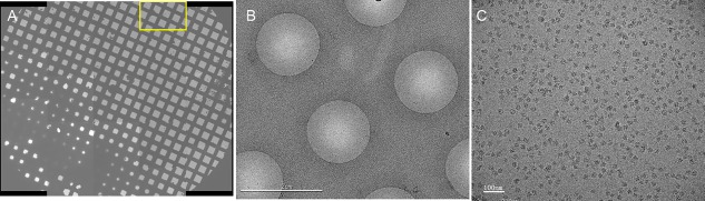
Cryo‐EM of T. cruzi ribosome. (A) Overview of the grid indicates that the grid is good, containing thin ice. (B) Hole views, which is from the region marked by the yellow box in A, reveal thin vitreous ice; the black spots within the hole are the ribosome particles. (C) Ribosome particle distribution on a micrograph.

Image Processing

Overview

The complete image processing workflow for single‐particle cryo‐EM usually contains particle selection, determination of the parameters of the CTF, determination of angles and positions (3D projection matching), 3D classification, and 3D reconstruction. Since the advent of the first‐single particle analysis software package—SPIDER 26 in the early 80s – a number of software packages have been developed, including IMAGIC,27 EMAN,28 XMIPP,29 BSOFT,30 SPARX,31 Frealign,32 and RELION 33 (For an exhaustive review, see https://en.wikibooks.org/wiki/Software_Tools_For_Molecular_Microscopy). Furthermore, two entire software platforms have been developed from which individual packages can be accessed interactively: Appion 34 and Scipion.35 Even though most popular packages provide standard and common pipelines to complete processing, each project may in fact require different strategies, depending on the properties of the sample. In the image processing of our T. cruzi ribosome dataset, multiple available packages such as SPIDER, EMAN, RELION, and so forth, have been utilized, as will be detailed below. In giving an overview, we distinguish two sections, pre‐processing conducted on a single desktop, and processing on a computer cluster (Fig. 2).

Figure 2.

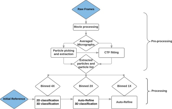
Overview of the image processing workflow for the T. cruzi data set.

Pre‐processing

Movie processing

A raw movie output from the electron microscope comprises multiple exposures (frames) of a single region of the sample grid. It can be recorded either in integrating mode by current versions of DE and Falcon or in counting mode by the K2 Summit camera. Whatever nature of the movies, they are amenable for correction of drift induced either by interacting electrons or by motions of the specimen stage. At present, the available drift correction algorithms include motioncorr (dosefgpu_driftcorr)7 and its successor motioncorr2, alignframes_lmbfgs and alignparts_lmbfgs,36 the optical Flow method in Xmipp,37 Unblur,38 and the particle polishing procedure in RELION.39 The micrographs or particles resulting from movie processing are subject to the traditional image processing pipeline.

The principle of these movie processing algorithms is that they first calculate the movements between the frames, compensate the offsets and sum over the shifted frames to yield the drift‐corrected dataset. Drift calculation and image summing may be done at different levels of the image: whole frame, sub‐frame, and particle. Motioncorr,7 the first popular movie processing software, relies on pair‐wise cross‐correlations to calculate translations at the whole‐frame level. The programs alignframes_lmbfgs and alignparts_lmbfgs 36 align either whole movie frames or individual particles, respectively. The Optical Flow approach37 estimates translations of frames or individual particles based on the representation of local motion by a vector field. Unblur 38 uses cross‐correlation iteratively to align each individual frame to an average of frames that does not include the frame being aligned. Particle polishing39 is an approach that corrects for particle movement using the 2D projections of a 3D reference map to align individual particles and thereby refine their positions.

In the image processing for the T. cruzi ribosome, movie processing was done on movies that were screened visually in advance. In our strategy, we first used motioncorr1 initially for averaging all frames of each micrograph and then ran the complete image processing workflow as outlined in Figure 2. At a later stage, described further below, the movie processing was revisited with different frame averaging combinations as it is known that earlier frames have more drift and later frames experience more radiation damage.7

CTF‐fitting

Bright‐field images obtained in the transmission electron microscope (TEM) are affected by the phase contrast transfer function (CTF).40 More specifically, the Fourier transform of the image is modulated in amplitude and flipped in phase in a spatial frequency‐dependent manner. This distorting effect can be corrected by restoring the actual Fourier amplitudes and phases for each micrograph. Among the parameters (defocus, B‐factor, astigmatism, etc.), the defocus value is the only one that can be controlled in the experiment, but its actual value always differs from the nominal one for several reasons, including precise sample height. As the most critical parameter to be determined, the defocus is estimated by fitting of a simulated power spectrum to the power spectrum of the electron micrograph. The fitting is facilitated by the characteristic signature of the CTF visible in the Fourier transform of the micrograph, known as Thon rings. The power spectrum is usually calculated by averaging absolute‐squared Fourier transforms of boxed particles or of selected sub‐regions of a micrograph.

To precisely determine defocus values, we used two methods, CTFFIND3,41 which uses the average of power spectra from boxed regions of the micrograph, and CTFIT2,42 which instead uses the average of power spectra of selected particles. The values obtained from both methods were cross‐validated. Only micrographs with matching defocus values (i.e., with a difference smaller than 50 nm) were kept for subsequent processing, while the remaining micrographs were subjected to visual verification and manual CTF fitting. Only those with well‐fitting CTF curves were returned to the processing workflow while the rest were discarded.

Data screening

Automatic imaging brings with it convenience in data collection but also an increase in the amount of contaminated or suboptimal data in the output dataset. Inevitably such a dataset requires more careful screening compared with data collected manually. Altogether we used four different strategies to screen the data at different steps in the workflow of image processing.

First, micrographs were examined visually to remove those with contamination by pieces of ice and ethane and those exposed to the shifted beam, before movie processing and particle picking. Second, micrographs with too few particles or showing areas of thick ice were excluded in a semi‐auto particle selection step using e2boxer.py.28 Third, power spectra of micrographs generated for CTF determination after movie processing were examined to exclude those with uncorrected drift and astigmatism. Fourth, as already noted above, inconsistencies among defocus values calculated by different CTF algorithms were used to reject some micrographs. In this manner, we ensured that only high‐quality micrographs proceeded to the image processing.

Processing

The processing step usually comprises 2D image alignment, 3D classification and reconstruction from hundreds of thousands to millions particle images, which requires a substantial amount of computational resources in terms of CPU time and memory. In our case, after pre‐screening, we set out with a total number of 700 k particles. This section in our work is divided into three successive steps performed on the 4× binned, 2× binned and 1× binned (i.e., un‐binned) dataset, respectively (Fig. 3).

Figure 3.

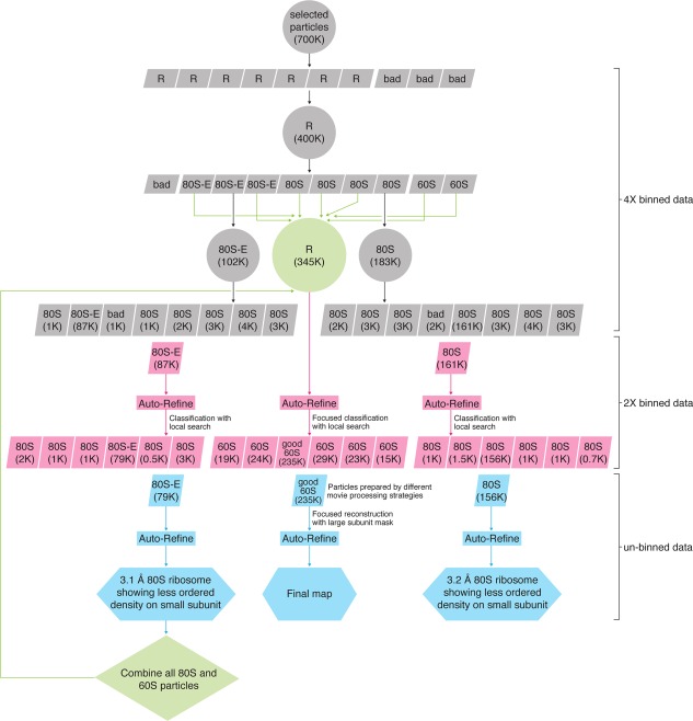
The entire workflow of the classification and reconstruction for T. cruzi data set. R, ribosome like class including both 80S and 60S; bad, bad class; 80S, class of empty 80S ribosomes; 80S‐E, class of 80S ribosomes with E‐site tRNA; 60S, class of 60S subunits.

Initial reference

To determine view angles and positions of the selected particles, an initial 3D low‐resolution reference is routinely used. From this reference a set of projections is generated for comparison with the raw (i.e., unprocessed) particles, and the angles and positions from the best matching projections are assigned to the particle. These initial parameters are further iteratively refined by comparing each particle with projections of the map reconstructed from the previous iteration, and so forth. Since strong low‐pass filtration is used to mitigate the effect of reference bias, the choice of initial reference is not critical; it may be derived from the cryo‐EM map of a loosely related structure, or from coordinates of a related structure deposited in the PDB database (http://www.rcsb.org/). In processing our T. cruzi dataset, we used a previously reconstructed cryo‐EM 70S ribosome structure17 filtered to 60 Å as the initial reference. The fact that our reconstruction displays no similarity to the 70S ribosome in its high‐resolution features indicates absence of reference bias.

Classifications on binned datasets

Because of the large degree of heterogeneity in single‐particle cryo‐EM data, classification is a hierarchical, multi‐stage procedure that requires careful consideration. It is a step that is difficult to automate, in part because strategic decisions that are dependent on the outcome at every level must be made in the process. Since the sorting progresses from coarse to fine details, it can be done on binned versions of the data first, to save time. In our case, we chose two stages of binning, 4× and 2×, before proceeding to the processing of un‐binned data. The entire workflow of classification at these three stages is schematically displayed in Figure 3.

On the 4× binned dataset, an initial step of 2D classification was used to eliminate impurities and “bad” particles in large part. This was followed by 3D RELION‐based classification run in a hierarchical way. The first round aimed at further cleaning the dataset resulting from screening by 2D classification, and obtain an inventory of existing conformations and compositions in the dataset, with K = 10 chosen as number of classes. As the sample had been obtained by purification from a cell extract without further intervention, is was uncertain at this stage which, if any, work cycle state of the ribosome would dominate, and could therefore be singled out in the subsequent image processing for high‐resolution structure determination.

For the second round of classification, all ribosome‐like particles (400 k) were pooled, and the number of classes was chosen to be higher (K = 10) than the number of ribosome‐like classes (K = 7) revealed in the first‐round classification. In this round, various states of the ribosome could be recognized, including whole ribosomes with/without bound components (tRNAs, eEF2), in rotated and un‐rotated configurations, and the two disassociated subunits. Two sizable classes of ribosomes without P‐site tRNA and GTPase factors were found, showing occupation by E‐site tRNA as the only difference.

The third‐round classification was applied to various sub‐groups, which were pooled based on similarity in the second‐round classification. The idea was that in this way, possible new classes of conformations not sorted out in the previous round of classification could be established, or, alternatively, the previous classification could be confirmed.

On the 2× binned data, refinement and reconstruction (Auto‐refine in RELION) was first performed on the two 80S classes with most particles obtained in the third‐ and last‐round classification of the 4× binned data. In one (87 k particles) the ribosome contained the E‐site tRNA; in the other (161 k particles) it was empty. The resulting reconstructed maps were then taken as references for 3D classification, this time using a finer local angular and translational search, of the same particles subset which generated this reconstruction. Here the rationale was that in this way, any deviant particles might be relegated to a less populated class and a more homogeneous subset would be obtained. This strategy worked: the two classes were whittled down to 79 k and 156 k, respectively.

Refinement and reconstruction of unbinned data

At this stage of the analysis, following a strategy that is now routine, auto‐refine in RELION may be used to generate a final 3D reconstruction from a homogeneous subpopulation of particles. However, there are many cases where a tailored, individual strategy is required to handle difficulties during imaging processing. Such difficulties arise when the structure in parts of the molecule is stable and reproducible, but flexible in other parts, and can be solved by application of a mask on the 3D map to single out regions of interest for further classification or refinement (“focused classification” or “focused reconstruction,” respectively43). In our case, the residual heterogeneity of the small subunit in the 80S ribosome classes compromised the resolution that could be obtained for the large subunit. Application of Auto‐refine on the two fixed subpopulations produced maps of the 80S ribosome with the overall resolutions of 3.1 Å and 3.2 Å, respectively.

At the next stage we made the decision to focus on the large subunit only in the subsequent refinement. We went back to the entire pool of 345 k particles identified as 80S and 60S in the second round of the classification of 4× binned data, and used the 3.1 Å 80S reconstruction with mask passing the 60S subunit as reference in a focused classification of this pooled dataset, yielding 2.9 Å resolution. Next, to obtain a refined reconstruction at highest resolution, the reconstruction for the pooled subset was made to revisit the particles extracted from micrographs generated for different choices frame averaging. We tried the following combinations: 2–10, 3–10, 4–10, 2–11, 3–11, and 4–11, and obtained the best result (2.5 Å) with frames 3–10.

Resolution Estimation and Modeling

Resolution estimation

In X‐ray or electron crystallography, the extent of the diffraction pattern (i.e., the radius in reciprocal space up to which diffraction peaks are detected) is an indicator of resolution. No equivalent criterion exists that would indicate the resolution of signal contained in the raw data for the single‐particle cryo‐EM method. Instead, resolution is estimated based on reproducibility of the reconstruction from independent datasets. The Fourier shell correlation (FSC) between the reconstructions of two half‐sets that have been refined independently eliminates in large part the bias from over‐fitted noise. When independence is thus ensured, the spatial frequency at the cutoff of FSC = 0.143 is regarded as a measure of resolution.44

In the use of FSC to estimate resolution from two maps, a mask is applied to the two maps before calculation of the FSC. Purpose of the mask is to screen off irreproducible peripheral density and noise45 that, if admitted, would lead to underestimation of resolution. In our case, flexible expansion segments (ES) and some extended proteins in the periphery needed to be masked off for a realistic resolution estimation of the reconstruction. We used a RELION‐tailored mask choosing a threshold such that well‐ordered regions of the ribosome were included, with a smooth 3‐pixel wide edge falloff. Specifically, our mask excludes the L1 and P stalk proteins, as well as some long ribosomal RNA expansion segments (Fig. 4).

Figure 4.

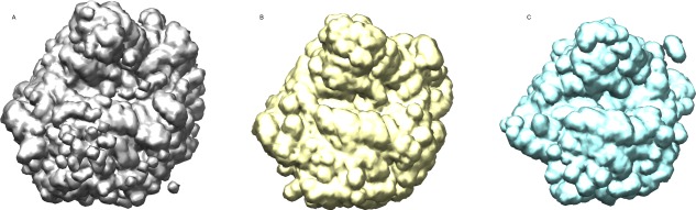
Masks for resolution estimation of T. cruzi cryo‐EM reconstruction. (A) A mask including all the components of the 60S subunit and some residual density from the small subunit. (B) A mask used in focus refinement, encompassing only the 60S subunit. (C) The mask used for resolution estimation, eliminating flexible components such as the P stalk.

In addition to the fixed number provided by the FSC method, local resolution estimation is quite informative since the definition of features varies substantially across the map. In our work, we estimated local resolution of our large subunit map using the software Resmap,46 and found it to range from 2.3 Å in the core region to 4.5 Å to in the periphery (Fig. 6).

Figure 6.

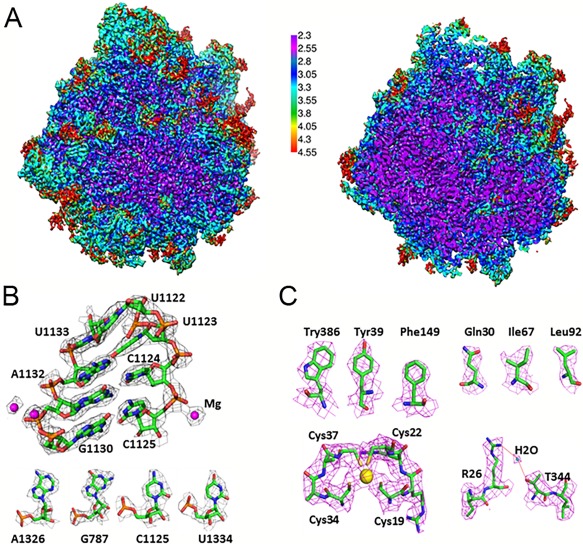
High‐resolution structure of the T. cruzi 60S ribosomal subunit. (A) Cryo‐EM map of the 60S subunit after sharpening, colored by local resolution and viewed from the subunit interface. Left, surface view; right, central cut‐away view. (B) Cryo‐EM density of a highlighted rRNA region of LSU‐α docked with atomic model. Bottom panel, examples for the four nucleotides in rRNA. (C) Selected views of the density maps of proteins. Top, densities for some of the amino acids. Bottom left, density of a zinc ion; Bottom right, density of a water molecule.

Modeling

Typically, the cryo‐EM map of a macromolecular complex is a chimera composed of regions with highly variable resolution, and a single overall resolution figure cannot do justice to this situation. Therefore, unlike X‐ray crystallography where model‐building and refinement strategies are chosen on the basis of the overall resolution,47 cryo‐EM often requires multi‐map modeling and refinement. In the case of the T. cruzi ribosome structure, such a multi‐map modeling strategy was also used (Fig. 5). Three density maps were generated by sharpening the initial map with negative B‐factors of −30 Ų, −50 Ų, and −75 Ų. The resulting maps were combined, taking advantage of the fact that they complemented one another in connectivity and definition of high‐resolution features. Before being loaded into the Coot modeling software,43 the maps (originally 400 × 400 × 400) were cropped to a size (230 × 230 × 230, with the spacing at 1.045 Å/voxel) just large enough to contain the whole large subunit, so as to keep within the bounds of the computer memory.

Figure 5.

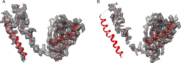
Protein eL31 after sharpening with different negative B factors. (A) B = −30 Ų. (B) B = −75 Ų. The missing density on the left helix of eL31 is caused by sharpening with a larger B factor, −75 Ų. The display of the figures is set at 3 × σ.

The high‐resolution features of the density map and the sequence information of the T. cruzi ribosome allowed us to register the rRNA and protein residues with well‐ordered blocks of density (Fig. 6B,C). In most of the density regions (approximately 85%) our map was of sufficient quality to allow de novo modeling as routinely done in X‐ray crystallography. However, to simplify and accelerate our modeling work, we took advantage of the extent of sequence identity and structural conservation between the T. cruzi ribosome and the previously studied yeast and T. brucei ribosomes. First the crystal structure of the yeast large ribosomal subunit (PDB: 4V88)48 and the structure of T. brucei large ribosomal subunit (PDB: 4V8M)1 were fitted into the density map as a rigid bodies using UCSF Chimera.49 The conserved regions matched the density map well after real space refinement. Regions of rRNA conserved between T. cruzi and yeast were used as starting points, followed by extensive manual building using Coot.50 In the non‐conserved rRNA regions, which account for more than half of the rRNA of the large subunit, the distinguishable side chain features for the bases, application of the base‐pairing principle, and the sequence information of the T. cruzi strain used allowed us to register each of the well‐resolved bases. The rRNA sequences were obtained from TriTrypDB Kinetoplastid Genomics Resource (http://tritrypdb.org/tritrypdb/).51 For the modeling of the non‐conserved regions of proteins, the polypeptide chains in T. brucei were mutated to match their sequences in T. cruzi taken from the National Center for Biotechnology Information (NCBI) protein databases (http://www.ncbi.nlm.nih.gov). On account of the fact that the fitted PDB of T. brucei was derived from a 5.5‐Å cryo‐EM map (EMD‐2239), some assignments of amino acid residues were found to be offset and inaccurate. In our density map, the high‐resolution features of the residue side‐chain density map allowed us to correct these assignments and also extend the peptide chains for the non‐conserved regions of proteins. Interestingly, some residue densities reveal inconsistencies with the residues from the T. cruzi sequence in the database, a reflection of natural mutations. For example, in our structure, residue 64 in protein eL37 is a Cys in the sequence of the database, but clearly a Met based on the density.6 The resultant atomic model of the large ribosomal subunit was subjected to real‐space refinement using PHENIX 52 against the map generated by sharpening with the negative B factor of −50 Ų.

Perspective

The foregoing outline of methods and choices of processing paths that we used in the determination of T. cruzi ribosome structure will make it clear that even with a given high‐quality dataset, achievement of highest resolution by single‐particle cryo‐EM is far from routine; that it requires a good knowledge of the principles underlying data processing and a good deal of intuition. Heterogeneity is a particularly vexing problem that often requires trial and error approaches that rarely make it into the formal Methods descriptions of scientific articles.

The last three years have witnessed spectacular achievements of biological macromolecules structure determination by single‐particle cryo‐EM. Among novel biological insights that have been gained are the mechanism of transcription initiation53 and the activation and gating of the calcium release channel,23, 54 which are refractory to structure characterization by traditional methods. Certain samples, such as ribosomes and viruses, are now rarely pursued using X‐ray crystallography as cryo‐EM needs fewer samples and works with higher efficiency. Even more promise lies in the near future since sample preparation, instrumentation, and computer software are all under development by the cryo‐EM community. In the study of ribosomes, usage of high magnification with finer pixel size, electron counting cameras, and anisotropic scale correction in image processing might further enhance the resolution to beyond 2 Å, which has already been realized on a small molecule.55

References

- 1. Hashem Y, des Georges A, Fu J, Buss SN, Jossinet F, Jobe A, Zhang Q, Liao HY, Grassucci RA, Bajaj C, Westhof E, Madison‐Antenucci S, Frank J (2013) High‐resolution cryo‐electron microscopy structure of the Trypanosoma brucei ribosome. Nature 494:385–389. [DOI] [PMC free article] [PubMed] [Google Scholar]
- 2. Armache JP, Jarasch A, Anger AM, Villa E, Becker T, Bhushan S, Jossinet F, Habeck M, Dindar G, Franckenberg S, Marquez V, Mielke T, Thomm M, Berninghausen O, Beatrix B, Soding J, Westhof E, Wilson DN, Beckmann R (2010) Cryo‐EM structure and rRNA model of a translating eukaryotic 80S ribosome at 5.5‐A resolution. Proc Natl Acad Sci USA 107:19748–19753. [DOI] [PMC free article] [PubMed] [Google Scholar]
- 3. Shalev‐Benami M, Zhang Y, Matzov D, Halfon Y, Zackay A, Rozenberg H, Zimmerman E, Bashan A, Jaffe CL, Yonath A, Skiniotis G (2016) 2.8‐Å cryo‐EM structure of the large ribosomal subunit from the eukaryotic parasite Leishmania. Cell Rep 16:288–294. [DOI] [PMC free article] [PubMed] [Google Scholar]
- 4. Passos DO, Lyumkis D (2015) Single‐particle cryoEM analysis at near‐atomic resolution from several thousand asymmetric subunits. J Struct Biol 192:235–244. [DOI] [PubMed] [Google Scholar]
- 5. Fischer N, Neumann P, Konevega AL, Bock LV, Ficner R, Rodnina MV, Stark H (2015) Structure of the E. coli ribosome‐EF‐Tu complex at <3 Å resolution by Cs‐corrected cryo‐EM. Nature 520:567–570. [DOI] [PubMed] [Google Scholar]
- 6. Liu Z, Gutierrez‐Vargas C, Wei J, Grassucci RA, Ramesh M, Espina N, Sun M, Tutuncuoglu B, Madison‐Antenucci S, Woolford JL, Tong L, Frank J (2016) Structure and assembly model for the Trypanosoma cruzi 60S ribosomal subunit. Proc Natl Acad Sci USA doi:10.1073/pnas.1614594113. [DOI] [PMC free article] [PubMed] [Google Scholar]
- 7. Li X, Mooney P, Zheng S, Booth CR, Braunfeld MB, Gubbens S, Agard DA, Cheng Y (2013) Electron counting and beam‐induced motion correction enable near‐atomic‐resolution single‐particle cryo‐EM. Nat Methods 10:584–590. [DOI] [PMC free article] [PubMed] [Google Scholar]
- 8. Yonekura K, Braunfeld MB, Maki‐Yonekura S, Agard DA (2006) Electron energy filtering significantly improves amplitude contrast of frozen‐hydrated protein at 300 kV. J Struct Biol 156:524–536. [DOI] [PubMed] [Google Scholar]
- 9. Danev R, Baumeister W (2016) Cryo‐EM single particle analysis with the Volta phase plate. Elife 5:e13046. [DOI] [PMC free article] [PubMed] [Google Scholar]
- 10. Frank J (2009) Single‐particle reconstruction of biological macromolecules in electron microscopy‐30 years. Q Rev Biophys 42:139–158. [DOI] [PMC free article] [PubMed] [Google Scholar]
- 11. Kudryashev M, Castano‐Diez D, Stahlberg H (2012) Limiting factors in single particle cryo electron tomography. Comput Struct Biotechnol J 1:e201207002. [DOI] [PMC free article] [PubMed] [Google Scholar]
- 12. Grigorieff N, Harrison SC (2011) Near‐atomic resolution reconstructions of icosahedral viruses from electron cryo‐microscopy. Curr Opin Struct Biol 21:265–273. [DOI] [PMC free article] [PubMed] [Google Scholar]
- 13. Liu Z, Guo F, Wang F, Li TC, Jiang W (2016) 9 A resolution cryo‐EM 3D reconstruction of close‐packed virus particles. Structure 24:319–328. [DOI] [PMC free article] [PubMed] [Google Scholar]
- 14. Guo F, Liu Z, Fang PA, Zhang Q, Wright ET, Wu W, Zhang C, Vago F, Ren Y, Jakana J, Chiu W, Serwer P, Jiang W (2014) Capsid expansion mechanism of bacteriophage T7 revealed by multistate atomic models derived from cryo‐EM reconstructions. Proc Natl Acad Sci USA 111:E4606–E4614. [DOI] [PMC free article] [PubMed] [Google Scholar]
- 15. Zhang X, Zhou ZH (2011) Limiting factors in atomic resolution cryo electron microscopy: no simple tricks. J Struct Biol 175:253–263. [DOI] [PMC free article] [PubMed] [Google Scholar]
- 16. Liu Z, Zhang J‐J (2014) Revolutionary breakthrough of structure determination—recent advances of electron direct detection device application in cryo‐EM. Acta Biophysica Sinica 30:1–12. [Google Scholar]
- 17. Li W, Liu Z, Koripella RK, Langlois R, Sanyal S, Frank J (2015) Activation of GTP hydrolysis in mRNA‐tRNA translocation by elongation factor G. Sci Adv 1. Vol. 1, no. 4, e1500169:1–7. [DOI] [PMC free article] [PubMed] [Google Scholar]
- 18. Lei JL, Frank J (2005) Automated acquisition of cryo‐electron micrographs for single particle reconstruction on an FEI Tecnai electron microscope. J Struct Biol 150:69–80. [DOI] [PubMed] [Google Scholar]
- 19. Zhang JJ, Nakamura N, Shimizu Y, Liang N, Liu X, Jakana J, Marsh MP, Booth CR, Shinkawa T, Nakata M, Chiu W (2009) JADAS: a customizable automated data acquisition system and its application to ice‐embedded single particles. J Struct Biol 165:1–9. [DOI] [PMC free article] [PubMed] [Google Scholar]
- 20. Suloway C, Shi J, Cheng A, Pulokas J, Carragher B, Potter CS, Zheng SQ, Agard DA, Jensen GJ (2009) Fully automated, sequential tilt‐series acquisition with Leginon. J Struct Biol 167:11–18. [DOI] [PMC free article] [PubMed] [Google Scholar]
- 21. Mastronarde DN (2005) Automated electron microscope tomography using robust prediction of specimen movements. J Struct Biol 152:36–51. [DOI] [PubMed] [Google Scholar]
- 22. Li XM, Zheng S, Agard DA, Cheng YF (2015) Asynchronous data acquisition and on‐the‐fly analysis of dose fractionated cryoEM images by UCSFImage. J Struct Biol 192:174–178. [DOI] [PMC free article] [PubMed] [Google Scholar]
- 23. Zalk R, Clarke OB, des Georges A, Grassucci RA, Reiken S, Mancia F, Hendrickson WA, Frank J, Marks AR (2015) Structure of a mammalian ryanodine receptor. Nature 517:44–U49. [DOI] [PMC free article] [PubMed] [Google Scholar]
- 24. Bai XC, Rajendra E, Yang G, Shi Y, Scheres SH (2015) Sampling the conformational space of the catalytic subunit of human gamma‐secretase. Elife 4:e11182. [DOI] [PMC free article] [PubMed] [Google Scholar]
- 25. Sun M, Li W, Blomqvist K, Das S, Hashem Y, Dvorin JD, Frank J (2015) Dynamical features of the Plasmodium falciparum ribosome during translation. Nucleic Acids Res 43:10515–10524. [DOI] [PMC free article] [PubMed] [Google Scholar]
- 26. Frank J, Radermacher M, Penczek P, Zhu J, Li Y, Ladjadj M, Leith A (1996) SPIDER and WEB: processing and visualization of images in 3D electron microscopy and related fields. J Struct Biol 116:190–199. [DOI] [PubMed] [Google Scholar]
- 27. van Heel M, Harauz G, Orlova EV, Schmidt R, Schatz M (1996) A new generation of the IMAGIC image processing system. J Struct Biol 116:17–24. [DOI] [PubMed] [Google Scholar]
- 28. Tang G, Peng L, Baldwin PR, Mann DS, Jiang W, Rees I, Ludtke SJ (2007) EMAN2: an extensible image processing suite for electron microscopy. J Struct Biol 157:38–46. [DOI] [PubMed] [Google Scholar]
- 29. Sorzano COS, Marabini R, Velazquez‐Muriel J, Bilbao‐Castro JR, Scheres SHW, Carazo JM, Pascual‐Montano A (2004) XMIPP: a new generation of an open‐source image processing package for electron microscopy. J Struct Biol 148:194–204. [DOI] [PubMed] [Google Scholar]
- 30. Heymann JB (2001) Bsoft: image and molecular processing in electron microscopy. J Struct Biol 133:156–169. [DOI] [PubMed] [Google Scholar]
- 31. Hohn M, Tang G, Goodyear G, Baldwin PR, Huang Z, Penczek PA, Yang C, Glaeser RM, Adams PD, Ludtke SJ (2007) SPARX, a new environment for Cryo‐EM image processing. J Struct Biol 157:47–55. [DOI] [PubMed] [Google Scholar]
- 32. Grigorieff N (2007) FREALIGN: high‐resolution refinement of single particle structures. J Struct Biol 157:117–125. [DOI] [PubMed] [Google Scholar]
- 33. Scheres SH (2012) A Bayesian view on cryo‐EM structure determination. J Mol Biol 415:406–418. [DOI] [PMC free article] [PubMed] [Google Scholar]
- 34. Lander GC, Stagg SM, Voss NR, Cheng A, Fellmann D, Pulokas J, Yoshioka C, Irving C, Mulder A, Lau PW, Lyumkis D, Potter CS, Carragher B (2009) Appion: an integrated, database‐driven pipeline to facilitate EM image processing. J Struct Biol 166:95–102. [DOI] [PMC free article] [PubMed] [Google Scholar]
- 35. de la Rosa‐Trevin JM, Quintana A, Del Cano L, Zaldivar A, Foche I, Gutierrez J, Gomez‐Blanco J, Burguet‐Castell J, Cuenca‐Alba J, Abrishami V, Vargas J, Oton J, Sharov G, Vilas JL, Navas J, Conesa P, Kazemi M, Marabini R, Sorzano CO, Carazo JM (2016) Scipion: a software framework toward integration, reproducibility and validation in 3D electron microscopy. J Struct Biol 195:93–99. [DOI] [PubMed] [Google Scholar]
- 36. Rubinstein JL, Brubaker MA (2015) Alignment of cryo‐EM movies of individual particles by optimization of image translations. J Struct Biol 192:188–195. [DOI] [PubMed] [Google Scholar]
- 37. Abrishami V, Vargas J, Li XM, Cheng YF, Marabini R, Sorzano COS, Carazo JM (2015) Alignment of direct detection device micrographs using a robust Optical Flow approach. J Struct Biol 189:163–176. [DOI] [PubMed] [Google Scholar]
- 38. Grant T, Grigorieff N (2015) Measuring the optimal exposure for single particle cryo‐EM using a 2.6 angstrom reconstruction of rotavirus VP6. Elife 4:e06980. [DOI] [PMC free article] [PubMed] [Google Scholar]
- 39. Scheres SH (2014) Beam‐induced motion correction for sub‐megadalton cryo‐EM particles. Elife 3:e03665. [DOI] [PMC free article] [PubMed] [Google Scholar]
- 40. Wade RH, Frank J (1977) Electron‐microscope transfer‐functions for partially coherent axial illumination and chromatic defocus spread. Optik 49:81–92. [Google Scholar]
- 41. Mindell JA, Grigorieff N (2003) Accurate determination of local defocus and specimen tilt in electron microscopy. J Struct Biol 142:334–347. [DOI] [PubMed] [Google Scholar]
- 42. Jiang W, Guo F, Liu Z (2012) A graph theory method for determination of cryo‐EM image focuses. J Struct Biol 180:343–351. [DOI] [PMC free article] [PubMed] [Google Scholar]
- 43. Brown A, Amunts A, Bai XC, Sugimoto Y, Edwards PC, Murshudov G, Scheres SH, Ramakrishnan V (2014) Structure of the large ribosomal subunit from human mitochondria. Science 346:718–722. [DOI] [PMC free article] [PubMed] [Google Scholar]
- 44. Henderson R, Sali A, Baker ML, Carragher B, Devkota B, Downing KH, Egelman EH, Feng Z, Frank J, Grigorieff N, Jiang W, Ludtke SJ, Medalia O, Penczek PA, Rosenthal PB, Rossmann MG, Schmid MF, Schroder GF, Steven AC, Stokes DL, Westbrook JD, Wriggers W, Yang H, Young J, Berman HM, Chiu W, Kleywegt GJ, Lawson CL (2012) Outcome of the first electron microscopy validation task force meeting. Structure 20:205–214. [DOI] [PMC free article] [PubMed] [Google Scholar]
- 45. LeBarron J, Grassucci RA, Shaikh TR, Baxter WT, Sengupta J, Frank J (2008) Exploration of parameters in cryo‐EM leading to an improved density map of the E. coli ribosome. J Struct Biol 164:24–32. [DOI] [PMC free article] [PubMed] [Google Scholar]
- 46. Kucukelbir A, Sigworth FJ, Tagare HD (2014) Quantifying the local resolution of cryo‐EM density maps. Nat Methods 11:63–65. [DOI] [PMC free article] [PubMed] [Google Scholar]
- 47. Brown A, Long F, Nicholls RA, Toots J, Emsley P, Murshudov G (2015) Tools for macromolecular model building and refinement into electron cryo‐microscopy reconstructions. Acta Cryst D71:136–153. [DOI] [PMC free article] [PubMed] [Google Scholar]
- 48. Ben‐Shem A, de Loubresse NG, Melnikov S, Jenner L, Yusupova G, Yusupov M (2011) The structure of the eukaryotic ribosome at 3.0 angstrom resolution. Science 334:1524–1529. [DOI] [PubMed] [Google Scholar]
- 49. Pettersen EF, Goddard TD, Huang CC, Couch GS, Greenblatt DM, Meng EC, Ferrin TE (2004) UCSF chimera—a visualization system for exploratory research and analysis. J Comput Chem 25:1605–1612. [DOI] [PubMed] [Google Scholar]
- 50. Emsley P, Cowtan K (2004) Coot: model‐building tools for molecular graphics. Acta Cryst D60:2126–2132. [DOI] [PubMed] [Google Scholar]
- 51. Aslett M, Aurrecoechea C, Berriman M, Brestelli J, Brunk BP, Carrington M, Depledge DP, Fischer S, Gajria B, Gao X, Gardner MJ, Gingle A, Grant G, Harb OS, Heiges M, Hertz‐Fowler C, Houston R, Innamorato F, Iodice J, Kissinger JC, Kraemer E, Li W, Logan FJ, Miller JA, Mitra S, Myler PJ, Nayak V, Pennington C, Phan I, Pinney DF, Ramasamy G, Rogers MB, Roos DS, Ross C, Sivam D, Smith DF, Srinivasamoorthy G, Stoeckert CJ Jr., Subramanian S, Thibodeau R, Tivey A, Treatman C, Velarde G, Wang H (2010) TriTrypDB: a functional genomic resource for the Trypanosomatidae. Nucleic Acids Res 38:D457–D462. 4 [DOI] [PMC free article] [PubMed] [Google Scholar]
- 52. Adams PD, Grosse‐Kunstleve RW, Hung LW, Ioerger TR, McCoy AJ, Moriarty NW, Read RJ, Sacchettini JC, Sauter NK, Terwilliger TC (2002) PHENIX: building new software for automated crystallographic structure determination. Acta Cryst D58:1948–1954. [DOI] [PubMed] [Google Scholar]
- 53. Yan C, Wan R, Bai R, Huang G, Shi Y (2016) Structure of a yeast activated spliceosome at 3.5 Å resolution. Science 353:904–911. [DOI] [PubMed] [Google Scholar]
- 54. des Georges A, Clarke OB, Zalk R, Yuan Q, Condon KJ, Grassucci RA, Hendrickson WA, Marks AR, Frank J (2016) Structural basis for gating and activation of RyR1. Cell 167:145–157 e117. [DOI] [PMC free article] [PubMed] [Google Scholar]
- 55. Merk A, Bartesaghi A, Banerjee S, Falconieri V, Rao P, Davis MI, Pragani R, Boxer MB, Earl LA, Milne JLS, Subramaniam S (2016) Breaking cryo‐EM resolution barriers to facilitate drug discovery. Cell 165:1698–1707. [DOI] [PMC free article] [PubMed] [Google Scholar]