Convex Banding of the Covariance Matrix

Abstract

We introduce a new sparse estimator of the covariance matrix for high-dimensional models in which the variables have a known ordering. Our estimator, which is the solution to a convex optimization problem, is equivalently expressed as an estimator which tapers the sample covariance matrix by a Toeplitz, sparsely-banded, data-adaptive matrix. As a result of this adaptivity, the convex banding estimator enjoys theoretical optimality properties not attained by previous banding or tapered estimators. In particular, our convex banding estimator is minimax rate adaptive in Frobenius and operator norms, up to log factors, over commonly-studied classes of covariance matrices, and over more general classes. Furthermore, it correctly recovers the bandwidth when the true covariance is exactly banded. Our convex formulation admits a simple and efficient algorithm. Empirical studies demonstrate its practical effectiveness and illustrate that our exactly-banded estimator works well even when the true covariance matrix is only close to a banded matrix, confirming our theoretical results. Our method compares favorably with all existing methods, in terms of accuracy and speed. We illustrate the practical merits of the convex banding estimator by showing that it can be used to improve the performance of discriminant analysis for classifying sound recordings.

1 Introduction

The covariance matrix is one of the most fundamental objects in statistics, and yet its reliable estimation is greatly challenging in high dimensions. The sample covariance matrix is known to degrade rapidly as an estimator as the number of variables increases, as noted more than four decades ago (see, e.g., Dempster 1972), unless additional assumptions are placed on the underlying covariance structure (see Bunea & Xiao 2014 for an overview). Indeed, the key to tractable estimation of a high-dimensional covariance matrix lies in exploiting any knowledge of the covariance structure. In this vein, this paper develops an estimator geared toward a covariance structure that naturally arises in many applications in which the variables are ordered. Variables collected over time or representing spectra constitute two subclasses of examples.

We observe an independent sample, X₁, …, X_n ∈ ℝ^p of mean zero random vectors with true population covariance matrix $\mathbb{E}[{\mathbf{X}}_i{\mathbf{X}}_i^T]={\sum }^{\ast }$. When the variables have a known ordering, it is often natural to assume that the dependence between variables is a function of the distance between variables’ indices. Common examples are in stationary time series modeling, where ${\sum }_{j,(j+h)}^{\ast }$ depends only on h, the lag of the series, with −K ≤ h ≤ K, for some K > 0. One can weaken this assumption, allowing $\{{\sum }_{j,(j+h)}^{\ast }:-K\le h\le K\}$ to depend on j, while retaining the assumption that the bandwidth K does not depend on j. Another typical assumption is that ${\sum }_{jk}^{\ast }=\text{Cov}(X_j,X_k)$ decreases with |j−k|. A simple example is the moving-average process, where it is assumed that ${\sum }_{jk}^{\ast }=0\mathrm{ if}|j-k|>K$ for some bandwidth parameter K, and a covariance matrix Σ^* with this structure is called banded. Likewise, in a first-order autoregressive model, the elements decay exponentially with distance from the main diagonal, ${\sum }_{jk}^{\ast }\propto {\beta }^{|j-k|}$, where |β| < 1, justifying the term “approximately banded” used to describe such a matrix.

More generally, banded or approximately banded covariance matrices can be used to model any generic vector (X₁, …, X_p)^T whose entries are ordered such that any entries that are more than K apart are uncorrelated (or at most very weakly correlated). This situation does not specify any particular decay or ordering of correlation strengths. It is noteworthy that K itself is unknown, and may depend on n or p or both.

A number of estimators have been proposed for this setting that outperform the sample covariance matrix, $\mathbf{S}=n^{-1}{\sum }_{i=1}^n({\mathbf{X}}_i-\overline{\mathbf{X}}){({\mathbf{X}}_i-\overline{\mathbf{X}})}^T$, where $\overline{\mathbf{X}}=n^{-1}{\sum }_{i=1}^n{\mathbf{X}}_i$. In this paper we will focus on the squared Frobenius ${\Vert \Vert }_F^2$ and operator $\Vert {\Vert }_{\mathit{op}}$ norms of the difference between estimators and the population matrix, as measures of performance. Assuming that the random vectors are sampled from a multivariate normal distribution and that both the largest and smallest eigenvalues of Σ^* are bounded from above and below by some constants, it has been shown that $\frac{1}{p}{\Vert \mathbf{S}-{\sum }^{\ast }\Vert }_F^2=O_P\left(\frac{p}{n}\right)$ and that ${\Vert \mathbf{S}-{\sum }^{\ast }\Vert }_{op}=O_P\left(p\sqrt{\frac{\log p}{n}}\right)$, neither of which can be close to zero for p > n because the bounds are tight; see, for example, Bunea & Xiao (2014). This can be rectified when one uses, instead, estimators that take into account the structure of Σ^*. For instance, Bickel & Levina (2008) introduced a class of banding and tapering estimators of the form

$${\widehat{\sum }}_{\mathbf{T}}=\mathbf{T}\ast \mathbf{S},$$ (1.1)

where T is a Toeplitz matrix and ∗ denotes Schur multiplication. When the matrix T is of the form T_jk = 1{|j − k| > K}, for a pre-specified K, one obtains what is referred to as the banded estimator. More general forms of T are allowed (Bickel & Levina 2008). The Frobenius and operator norm optimality of such estimators has been studied relative to classes of approximately banded population matrices discussed in detail in Section 4.2 below. Members of these classes are matrices with entries decaying with distance from the main diagonal at rate depending on the the sample size n and a parameter α > 0. The minimax lower bounds for estimation over these classes have been established, for both norms, in Cai et al. (2010). The banding estimator achieves them in both Frobenius norm (Bickel & Levina 2008) and operator norm (Xiao & Bunea 2014), and the same is true for a more general tapering estimator proposed in Cai et al. (2010). The common element of these estimators is that, while being minimax rate optimal, they are not minimax adaptive, in that their construction utilizes knowledge of α, which is typically not known in practice. Moreover, there is no guarantee that the banded estimators are positive definite, while this can be guaranteed via appropriate tapering.

Motivated by the desire to propose a rate-optimal estimator that does not depend on α, Cai & Yuan (2012) propose an adaptive estimator that partitions S into blocks of varying sizes, and then zeros out some of these blocks. They show that this estimator is minimax adaptive in operator norm, over a certain class of population matrices. The block-structure form of their estimator is an artifact of an interesting proof technique, which relates the operator norm of a matrix to the operator norm of a smaller matrix whose elements are the operator norms of blocks of the original matrix. The construction is tailored to obtaining optimality in operator norm, and the estimator leans heavily on the assumption of decaying covariance away from the diagonal. In particular, it automatically zeros out all elements far from the diagonal without regard to the data (so a covariance far from the diagonal could be arbitrarily large and still be set to zero). In this sense, the method is less data-adaptive than may be desirable and may suffer in situations in which the long-range dependence does not decay fast enough. In addition, as in the case of the banded estimators, this block-thresholded estimator cannot be guaranteed to be positive definite. If positive definiteness is desired, the authors note that one may project the estimator onto the positive semidefinite cone (however, this projection step would lose the sparsity of the original solution).

Other estimators with good practical performance, in both operator and Frobenius norm, have been proposed, notably the banded Cholesky and nested lasso methods of Rothman et al. (2010). These approaches involve regularizing the Cholesky factor via solving a series of least squares or weighted lasso problems. The resulting estimators are sparse and positive definite; however, to our knowledge a theoretical study of these estimators has not been conducted.

1.1 The convex banding estimator

In this work we introduce a new covariance estimator with the goal of bridging several gaps in the existing literature. Our contributions are as follows:

1. We construct a new estimator that is sparsely-banded and positive definite with high probability. Our estimator is the solution to a convex optimization problem, and, by construction, has a data-dependent bandwidth. We call our estimation procedure convex banding.

2. We propose an efficient algorithm for constructing this estimator and show that it amounts to the tapering of the sample covariance matrix by a data-dependent matrix. In constrast to previous tapering estimators, which require a fixed tapering matrix, this data-dependent tapering allows our estimator to adapt to the unknown bandwidth of the true covariance matrix.

3. We show that our estimator is minimax rate adaptive (up to logarithmic factors) with respect to the Frobenius norm over a new class of population matrices that we term semi-banded. This class generalizes those of banded or approximately banded matrices. This establishes our estimator as the first with proved minimax rate adaptivity in Frobenius norm (up to logarithmic factors) over the previously studied covariance matrix classes. Moreover, members of the newly introduced class do not require entries to decay with the distance between their indices. This extends the scope of banded covariance estimators. We also show that our estimator is minimax rate optimal (again, up to logarithmic factors) and adaptive with respect to the operator norm over a class of matrices with elements close to banded matrices, with bandwidth that can grow with n, p or both, at an appropriate rate. Moreover, we show that our estimator recovers the underlying sparsity pattern with high probability.

An unusual (and favorable) aspect of our estimator is that it is simultaneously sparse and positive definite with high probability—a property not shared by any other method with comparable theoretical guarantees.

The precise definition of our convex banding estimator and a discussion of the algorithm are given in Sections 2 and 3 below. Our target Σ^* either has all elements beyond a certain bandwidth K being zero or it is close (in a sense defined precisely in Section 4) to a K-banded matrix. We therefore aim at constructing an estimator that will zero out all covariances that are beyond a certain data-dependent bandwidth. If we regard the elements we would like to set to zero as a group, it is natural to consider a penalized estimator, with a penalty that zeros out groups. The most basic penalty that sets groups of parameters to zero simultaneously, without any other restrictions on these parameters, is known as the Group Lasso (Yuan & Lin 2006), a generalization of the Lasso (Tibshirani 1996). Zhao et al. (2009) show that by taking a hierarchically-nested group structure, one can develop penalties that set one group of parameters to zero whenever another group is zero. Penalties that render various hierarchical sparsity patterns have been proposed and studied in, for instance, Jenatton et al. (2010), Radchenko & James (2010), Bach et al. (2012), Bien et al. (2013). The most common applications considered in these works are to regression models.

The convex banding estimator employs a new hierarchical group structure that is tailored to covariance matrices with a banded or semi-banded structure; its optimal properties cannot be obtained from simple extensions of any of the existing related penalties. We discuss this in Sections 2.1 and 4. We also provide a connection between our convex banded estimator and tapering estimators. Section 3.1 shows that our estimator can also be written in the form (1.1), but where T is a data-driven, sparse tapering matrix, with entries given by a data-dependent recursion formula, not a pre-specified, non-random, tapering function. This representation has both practical and theoretical implications: it allows us to compute our estimator efficiently, relate our estimator to previous banded or tapered estimators, and establish that it is banded and positive definite with high probability. These issues are treated in Sections 3.1 and 4.3, respectively.

In Section 4.1, we prove that, when the population covariance matrix is itself a banded matrix, our estimator recovers the sparsity pattern, under minimal signal strength conditions, which are made possible by the fact that we employ a hierarchical penalty. In Section 4.2 we show that our convex banding estimator is minimax rate adaptive, in both Frobenius and operator norms, up to multiplicative logarithmic factors, over appropriately defined classes of population matrices. In Section 5, we perform a thorough simulation study that investigates the sharpness of our bounds and demonstrates that our estimator compares favorably to previous methods. We conclude with a real data example in which we show that using our estimate of the covariance matrix leads to improved classification accuracy in both quadratic and linear discriminant analysis.

2 The definition of the convex banding estimator

To describe our estimator, we must begin by defining a set of groups that will induce the desired banded-sparsity pattern. We define

$$g_{\ell }=\{jk\in {[p]}^2:|j-k|\ge p-\ell \}$$

to be the two right triangles of indices formed by taking the ℓ(ℓ + 1) indices that are farthest from the main diagonal of a p × p matrix. See the left panel of Figure 1 for a depiction of g₃ when p = 5. For notational ease we will denote, as above, jk = (j, k), and [p]² = {1, …, p} × {1 …, p}.

Figure 1.

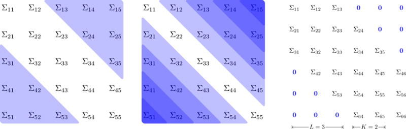
(Left) The group g₃; (Middle) the nested groups in the penalty (2.1); (Right) a K-banded matrix where K = 2 and p = 6. Note that L = p − K − 1 = 2 counts the number of subdiagonals that are zero. This can be expressed as ${\sum }_{g_L}=0$ or ${\sum }_{s_{\ell }}=0$ for 1 ≤ ℓ ≤ L.

We will also find it useful to express these groups as a union of subdiagonals s_m:

$$g_{\ell }={\displaystyle \underset{m=1}{\overset{\ell }{\cup }}{s}_m}\text{where}{s}_m=\{jk:|j-k|=p-m\}.$$

For example, g₁ = s₁ = {(1, p), (p, 1)} and, at the opposite extreme, $g_{p-1}^c=s_p$ is the diagonal. While the indexing of g_ℓ and s_m may at first seem “backwards” (in the sense that we count them from the outside-in rather than from the diagonal-out), our indexing is natural here because |s_m| = 2m and g_ℓ consists of two equilateral triangles with side-lengths of ℓ elements. The right panel of Figure 1 depicts the nested group structure: g₁ ⊂ ⋯ ⊂ g_p−1, where this largest group contains all off-diagonal elements.

The following notation is used in the definition of our estimator below. Given a subset of matrix indices g ⊆ [p]² of a p × p matrix Σ, let Σ_g ∈ ℝ^|g| be the vector with elements {Σ_jk : jk ∈ g}. For a given non-negative sequence of weights w_ℓm with 1 ≤ m ≤ ℓ ≤ p − 1, discussed in the following sub-section, and for a given λ ≥ 0, let $\widehat{\sum }$ be defined as the solution to the following convex optimization problem:

$$\widehat{\sum }=\arg \underset{\sum }{min}\left\{\frac{1}{2}{\Vert \sum -\mathbf{S}\Vert }_F^2+\lambda {\Vert \sum \Vert }_{2,1}^{\ast }\right\},$$ (2.1)

where ‖·‖_F is the Frobenius norm and

$${\Vert \sum \Vert }_{2,1}^{\ast }={\displaystyle \sum _{\ell -1}^{p-1}\sqrt{{\displaystyle \sum _{m-1}^{\ell }{w}_{\ell m}^2{\Vert {\sum }_{s_m}\Vert }_2^2}}}={\displaystyle \sum _{\ell =1}^{p-1}{\Vert {({\mathbf{W}}^{(\ell )}\ast \sum )}_{g\ell }\Vert }_2.}$$ (2.2)

Our penalty term is a weighted group lasso, using {g_ℓ : 1 ≤ ℓ ≤ p−1} as the group structure. For the second equality, we express the penalty as the elementwise product, denoted by ∗, of Σ with a sequence of weight matrices, W^(ℓ), that are Toeplitz with ${\mathbf{W}}_{s_m}^{(\ell )}=w_{\ell m}{1}_{\{m\le \ell \}}\cdot {\mathbf{1}}_{2m}$.

Remark 1

Problem 2.1 is strictly convex, so $\widehat{\sum }$ is the unique solution.

Remark 2

As the tuning parameter λ is increased, subdiagonals of $\widehat{\sum }$ become exactly zero. As long as w_ℓm > 0 for all 1 ≤ m ≤ ℓ ≤ p − 1, the hierarchical group structure ensures that a subdiagonal will only be set to zero if all elements farther from the main diagonal are already zero. Thus, we get an estimated bandwidth, $\widehat{K}$, which satisfies ${\widehat{\sum }}_{g_{p-\widehat{K}-1}}=0$ and ${\widehat{\sum }}_{s_{p-\widehat{K}}}\ne 0$ (see Theorem 2 and Corollary 1 for details).

We refer to $\widehat{\sum }$ as the convex banding of the matrix S. We show in Section 4.3 that $\widehat{\sum }$ is positive definite with high probability. Empirically, we find that positive definiteness holds except in very extreme cases. Moreover, in Section 4.3 we propose a different version of convex banding that guarantees positive definiteness:

$$\sum ^{\sim }=\arg \underset{\sum �\delta {\mathbf{I}}_p}{min}\left\{\frac{1}{2}{\Vert \sum -\mathbf{S}\Vert }_F^2+\lambda {\Vert \sum \Vert }_{2,1}^{\ast }\right\}.$$ (2.3)

Of course when ${\lambda }_{min}(\widehat{\sum })\ge \delta$, the two estimators coincide.

2.1 The weight sequence w_ℓm

Since for each ℓ, the weight w_ℓm penalizes s_m, 1 ≤ m ≤ ℓ, and the subdiagonals s_m increase in size with m, we want to give the largest subdiagonals the largest weight. We will therefore choose weights with w_ℓℓ = max_1≤m≤ℓw_ℓm and will sometimes write w_ℓ:= w_ℓℓ. We consider three choices of weights that satisfy this property.

1. (Non-hierarchical) Group lasso penalty

Letting $w_{\ell m}=1_{\{\ell =m\}}\sqrt{2\ell }$, for 1 ≤ m ≤ ℓ, 1 ≤ ℓ ≤ p − 1 yields

$${\Vert \sum \Vert }_{2,1}^{\ast }={\displaystyle \sum _{\ell -1}^{p-1}\sqrt{2\ell }{\Vert {\sum }_{s_{\ell }}\Vert }_2}.$$ (2.4)

This is a traditional group lasso penalty that acts on subdiagonals, with weights $w_{\ell }=\sqrt{|s_{\ell }|}$. This penalty is not hierarchical, as each subdiagonal may be set to zero independently of the others. In Section 4.1 we show how failing to use a hierarchical penalty requires more stringent minimum signal conditions in order to correctly recover the true bandwidth of Σ^*. However, if the interest is in accurate estimation in Frobenius or operator norm of population matrices that are close to banded, we show in Section 4.2.1 that this estimator is minimax rate optimal, up to logarithmic factors, despite the fact that in finite samples it may fail to have the correct sparsity pattern.

2. Basic hierarchical penalty

If $w_{\ell m}=\sqrt{2\ell }$, for all m and ℓ, the penalty term becomes

$${\Vert \sum \Vert }_{2,1}^{\ast }={\displaystyle \sum _{\ell =1}^{p-1}\sqrt{2\ell }}{\Vert {\sum }_{g\ell }\Vert }_2,$$ (2.5)

which employs the same weight, $\sqrt{2\ell }$, as above, but now for a triangle g_ℓ. Recalling that |g_ℓ| = ℓ(ℓ+1), we note that this does not follow the common principle guiding weight choices in the (non-overlapping) group lasso literature of using $\sqrt{|g_{\ell }|}$. In Section 4.1, we show this choice of weights leads to consistent bandwidth selection under minimal conditions on the strength of the signal; however, we shall show that a more refined choice ensures rate optimal estimation of Σ^* with respect to either Frobenius or operator norm. The problem with this simple choice of weights stems from the fact that subdiagonals far from the main diagonal (small m) are excessively penalized (since they appear in p − m terms). To balance this overaggressive enforcement of hierarchy, one desires weights that decay with decreasing m within a fixed group g_ℓ and yet still exhibit the $\sqrt{2\ell }$ growth on w_ℓℓ.

3. General hierarchical penalty

Based on the considerations above, we take the following choice of weights:

$$w_{\ell m}=\frac{\sqrt{2\ell }}{\ell -m+1},\text{for}1\le m\le \ell ,1\le \ell \le p-1.$$ (2.6)

We will show in Sections 4.2.1 and 4.2.2 that the corresponding estimator is minimax rate adaptive, in Frobenius and operator norm, up to logarithmic factors, over appropriately defined classes of population covariance matrices.

Remark 3

We re-emphasize the difference between the weighting schemes considered above. The estimators corresponding to (2.5) and (2.6) will always impose the sparsity structure of a banded matrix, a fact that is apparent from Theorem 2 below. In contrast, the group lasso estimator (2.4), which is performed on each sub-diagonal separately, may fail to recover this pattern.

3 Computation and properties

The most common approach to solving the standard group lasso is blockwise coordinate descent (BCD). Tseng (2001) proves that when the nondifferentiable part of a convex objective is separable, BCD is guaranteed to solve the problem. While this separable structure is not present in (2.1), Jenatton et al. (2010) show that the dual of this problem does, meaning that BCD on the dual can be used.

Theorem 1

A dual of (2.1) is given by

$$\underset{{\mathrm{A}}^{(\ell )}\in {ℝ}^{p\times p}}{\text{Minimize}}\frac{1}{2}{\Vert \mathbf{S}-\lambda {\displaystyle \sum _{\ell -1}^{p-1}{\mathbf{W}}^{(\ell )}\ast {\mathbf{A}}^{(\ell )}}\Vert }_F^2\mathrm{s}\mathrm{.t}.{\Vert {\mathbf{A}}_{g_{\ell }}^{(\ell )}\Vert }_2\le 1,{\mathbf{A}}_{g_{{\ell }^c}}^{(\ell )}=0\text{for}1\le \ell \le p-1.$$ (3.1)

In particular, given a solution to the dual, (Â⁽¹⁾, …, Â^(p−1)), the solution to (2.1) is given by the primal-dual relation, $\widehat{\sum }=\mathbf{S}-\lambda {\sum }_{\ell =1}^{p-1}{\mathbf{W}}^{(\ell )}\ast {\widehat{\mathbf{A}}}^{(\ell )}$.

Proof

See Section A.1 of the supplementary materials.

Algorithm 1 gives a BCD algorithm for solving (3.1), which by the primal-dual relation in turn gives a solution to (2.1). The blocks correspond to each dual variable matrix. The update over each A^(ℓ) involves projection of a matrix ${\widehat{\mathbf{R}}}^{(\ell )}$ (defined in Algorithm 1) onto an ellipsoid, which amounts to finding ${\widehat{\nu }}_{\ell }$, a root of the univariate function h_ℓ(ν) − λ², where

$$h_{\ell }(\nu )={\displaystyle \sum _{m=1}^{\ell }\frac{w_{\ell m}^2}{{(w_{\ell m}^2+\nu )}^2}}{\Vert {\widehat{\mathbf{R}}}_{s_m}^{(\ell )}\Vert }^2.$$ (3.2)

We explain in Section A.2 of the supplementary materials the details of ellipsoid projection and observe that we can get ${\widehat{\nu }}_{\ell }$ in closed form for all but the last $\widehat{K}$ values of ℓ (where $\widehat{K}$ is the bandwidth of $\widehat{\sum }$). A remarkable feature of our algorithm is that only a single pass of BCD is required to reach convergence. This property is proved in Jenatton et al. (2011) and is a direct consequence of the nested group structure. When we use the simple weights (2.5), in which w_ℓm = w_ℓ, Algorithm 1 becomes extraordinarly simple and transparent:

1. Initialize $\widehat{\sum }\leftarrow \mathbf{S}$

2. For ℓ = 1, …, $p-1:{\widehat{\sum }}_{g_{\ell }}\leftarrow (1-{\lambda }_{w_{\ell }}/{\Vert {\widehat{\sum }}_{g_{\ell }}\Vert }_2)+{\widehat{\sum }}_{g_{\ell }}.$

In words, we start with the sample covariance matrix, and then work from the corners of the matrix inward toward the main diagonal. At each step, the next largest triangle-pair is group-soft-thresholded. If a triangle is ever set to zero, it will remain zero for all future steps. We will show that this simple weighting scheme admits exact bandwidth and pattern recovery in Section 4.1.

Algorithm 1 BCD on dual of Problem (2.1).

Inputs: S, λ, and weights matrices, W(ℓ). Initialize Â(ℓ) = 0 for all ℓ.

For ℓ = 1, …, p − 1:

• Compute ${\widehat{\mathbf{R}}}^{(\ell )}\leftarrow \mathbf{S}-\lambda {\sum }_{{\ell }^{\prime }=1}^{p-1}{W}^{({\ell }^{\prime })}\ast {\widehat{\mathbf{A}}}^{({\ell }^{\prime })}$  • For m ≤ ℓ, set ${\widehat{\mathbf{A}}}_{s_m}^{(\ell )}\leftarrow \frac{w_{\ell m}}{\lambda (w_{\ell m}^2+max\{{\widehat{\nu }}_{\ell },0\})}{\widehat{\mathbf{R}}}_{s_m}^{(\ell )}$ where ${\widehat{\nu }}_{\ell }$ satisfies ${\lambda }^2=h_{\ell }({\widehat{\nu }}_{\ell })$, as in (3.2).

$\{{\widehat{\mathbf{A}}}^{(\ell )}\}$ is a solution to (3.1) and ${\widehat{\mathbf{R}}}^{(p)}=\mathbf{S}-\lambda {\sum }_{\ell =1}^{p-1}{\mathbf{W}}^{(\ell )}\ast {\widehat{\mathbf{A}}}^{(\ell )}$ is the solution to (2.1).

3.1 Convex banding as a tapering estimator

The next result shows that $\widehat{\sum }$ can be regarded as a tapering estimator with a data-dependent tapering matrix. In Section 4, we will see that, in contrast to estimators that use a fixed tapering matrix, our estimator adapts to the unknown bandwidth of the true matrix Σ^*.

Theorem 2

The convex banding estimator, $\widehat{\sum }$, can be written as a tapering estimator with a Toeplitz, data-dependent tapering matrix, $\widehat{\sum }=\widehat{\mathbf{T}}\ast \mathbf{S}$:

$${\widehat{\mathbf{T}}}_{s_m}=\{\begin{array}{ll}{\mathbf{1}}_m& \mathit{for}m=p(\text{diagonal})\\ {\displaystyle {\prod }_{\ell =m}^{p-1}\frac{[{\widehat{\nu }}_{\ell }]+}{w_{\ell m}^2+[{\widehat{\nu }}_{\ell }]+}}{\mathbf{1}}_m& \mathit{for}1\le m\le p-1\end{array}$$

where ${\widehat{\nu }}_{\ell }$ satisfies ${\lambda }^2={\sum }_{m=1}^{\ell }\frac{w_{\ell m}^2}{{(w_{\ell m}^2+{\widehat{\nu }}_{\ell })}^2}{\Vert {\widehat{\mathbf{R}}}_{s_m}^{(\ell )}\Vert }^2$ and 1_m ∈ ℝ^m is the vector of ones.

Proof

See Section A.3 of supplementary materials.     □

The following result shows that, as desired, our estimator is banded.

Corollary 1

$\widehat{\sum }$ is a banded matrix with bandwidth $\widehat{K}=p-1-max\{\ell :{\widehat{\nu }}_{\ell }\le 0\}$.

Proof

By definition, ${\widehat{\nu }}_{p-1-\widehat{K}}\le 0$ and ${\widehat{\nu }}_{p-\widehat{K}}$, …, ${\widehat{\nu }}_{p-1}>0$. It follows from the theorem that ${\widehat{\mathbf{T}}}_{s_m}={0.1}_m$ for all $m\le p-1-\widehat{K}$ and ${[{\widehat{\mathbf{T}}}_{s_m}]}_i>0$ for $p-\widehat{K}\le m\le p-1$.     □

4 Statistical properties of convex banding

In this section, we study the statistical properties of the convex banding estimator. We begin by stating two assumptions that specify the general setting of our theoretical analysis.

Assumption 1

Let X = (X₁, …, X_p)^T. Assume $\mathbb{E}\mathbf{X}=\mathbf{0}$ and denote $\mathbb{E}{\mathbf{XX}}^T={\sum }^{\ast }$. We assume that each X_j is marginally sub-Gaussian: $\mathbb{E}\exp (t{X}_j/\sqrt{{\sum }_{jj}^{\ast }})\le \exp (C{t}^2)$ for all t ≥ 0 and for some constant C > 0 that is independent of j. Moreover, ${max}_j|{\sum }_{jj}^{\ast }|\le M,$ for some constant M > 0.

Assumption 2

The dimension p can grow with n at most exponentially in n: γ₀ log n ≤ log p ≤ γn, for some constants γ₀ > 0, γ > 0.

The requirement that p grow at least polynomially fast as a function of n is not necessary but it simplifies the results allowing us to write log p instead of log[max(p, n)]. In Section 4.1, we prove that our estimator recovers the true bandwidth of Σ^* with high probability assuming the nonzero values of Σ^* are large enough. We will demonstrate that our estimator can detect lower signals than what could be recovered by an estimator that does not enforce hierarchy, re-emphasizing the need for a hierarchical penalty. In Section 4.2, we show that our estimator is minimax adaptive, up to multiplicative logarithmic terms, with respect to both the operator and Frobenius norms. Our results hold either with high probability or in expectation, and are established over classes of population matrices defined in Sections 4.2.1 and 4.2.2, respectively.

We begin by introducing a random set, on which all our results hold. Fixing x > 0, let

$${\mathcal{A}}_x=\left\{\underset{1\le i,j\le p}{max}|{\mathbf{S}}_{ij}-{\sum }_{ij}^{\ast }|\le x\sqrt{\log p/n}\right\}.$$ (4.1)

The following lemma shows that this set has high probability.

Lemma 1

Under Assumptions 1 and 2, there exists a constant c > 0 such that for sufficiently large x > 0, $\mathbb{P}({\mathcal{A}}_x)\ge 1-c/p$.

Proof

See Section A.4 of the supplementary materials, proof of (A.4.1) of Theorem A.1.     □

Remark 4

1. Similar results exist in the literature (see, e.g., Ravikumar et al. 2011). Lemma 3 in Bickel & Levina (2008) is proved under a Gaussianity assumption coupled with the assumption that ‖Σ^*‖_op is bounded. Whereas inspection of the proof shows that the latter is not needed, we cannot quote this result directly for other types of design. The commonly employed assumptions of sub-Gaussianity are placed on the entire vector X = (X₁, …, X_p)^T and postulate that there exists τ > 0 such that $\mathbb{P}\{|{\mathrm{v}}^T(\mathbf{X}-\mathbb{E}(\mathbf{X}))|>t\}\le \exp \{-t^2/(2\tau )\}$, for all t > 0 and ‖v‖₂ = 1, (see, e.g., Cai & Zhou 2012). However, if such a τ exists, then ‖Σ^*‖_op ≤ τ. Lemma 1 above shows that a bound on ‖Σ^*‖_op can be avoided in the probability bounds regarding ${max}_{ij}|{\mathbf{S}}_{ij}-{\sum }_{ij}^{\ast }|$, and the distributional assumption can be weakened to marginals.

2. In the classical case in which p does not depend on n, one can modify the definition of the set ${\mathcal{A}}_x$ by replacing the factor log(p) by log[max(n, p)], and the result of Lemma 1 will continue to hold with probability 1 − c/ max(n, p), for a possibly different constant c.

4.1 Exact bandwidth recovery

Suppose Σ^* has bandwidth K, that is, for L = p−K−1, we have ${\sum }_{g_L}^{\ast }=0$ and ${\sum }_{s_{L+1}}^{\ast }\ne 0$ (see right panel of Figure 1). We prove in this section that under mild conditions our estimator $\widehat{\sum }$ correctly recovers K with high probability. The next theorem expresses the intuitive result that if λ is chosen sufficiently large, we will not over-estimate the true bandwidth.

Theorem 3

If $\lambda \ge x\sqrt{\log p/n}$ and $w_{\ell }=\sqrt{2\ell }$, then $\widehat{K}\le K$, on the set ${\mathcal{A}}_x$.

Proof

See Section A.5 of the supplementary materials.     □

For our estimator to be able to detect the full band, we must require that the “signal” be sufficiently large relative to the noise. In the next theorem we measure the size of the signal by the ℓ₂ norm of each sub-diagonal (scaled in proportion to the square root of its size, $w_{\ell }=\sqrt{2\ell }$) and the size of the noise by λ.

Theorem 4

If ${min}_{\ell \ge L+1}{\Vert {\sum }_{s_{\ell }}^{\ast }\Vert }_2/w_{\ell }>2\lambda$, where $\lambda \ge x\sqrt{\log p/n}$ and $w_{\ell }=\sqrt{2\ell }$, then $K\le \widehat{K}$, on the set ${\mathcal{A}}_x$.

Proof

See Section A.5 of the supplementary materials.     □

In typical high-dimensional statistical problems, the support set can generically be any subset and therefore one must require that each element in the support set be sufficiently large on its own to be detected. By contrast, in our current context we know that the support set is of the specific form {L + 1, …, p − 1}, for some unknown L. Thus, as long as the signal is sufficiently large at L + 1, one might expect that the signal could be weaker at subsequent elements of the support. In the next theorem we demonstrate this phenomenon by showing that when ${\sum }_{s_{L+1}}^{\ast }$ exceeds the threshold given in the previous theorem, it may “share the wealth” of this excess, relaxing the requirement on the size of ${\sum }_{s_{L+2}}^{\ast }$.

Theorem 5 (“Share the wealth”)

Suppose (for some γ > 0)

${\Vert {\sum }_{s_{L+1}}^{\ast }\Vert }_2=(2+\gamma )\lambda w_{L+1},\underset{\ell \ge L+3}{min}{\Vert {\sum }_{s_{\ell }}^{\ast }\Vert }_2/w_{\ell }>2\lambda ,{\Vert {\sum }_{s_{L+2}}^{\ast }\Vert }_2>\lambda w_{L+2}(1+\sqrt{1-{\gamma }^2})1_{\{\gamma <1\}}$

where $\lambda \ge x\sqrt{\log p/n}$ and $w_{\ell }=\sqrt{2\ell }$ and w_ℓ,ℓ ≥ w_ℓ+1,ℓ > 0, then $K\le \widehat{K}$ on the set ${\mathcal{A}}_x$.

Proof

See Section A.5 of the supplementary materials.     □

When γ = 0, Theorem 5 reduces to Theorem 4. However, as γ increases, the required size of ${\Vert {\sum }_{s_{L+2}}^{\ast }\Vert }_2$ decreases without preventing the bandwidth from being misestimated. In fact, for γ ≥ 1, there is no requirement on ${\sum }_{s_{L+2}}^{\ast }$ for bandwidth recovery. This robustness to individual subdiagonals being small is a direct result of our method being hierarchical.

Remark 5

1. By Lemma 1, $\mathbb{P}({\mathcal{A}}_x)>1-c/p$, under Assumption 1 and 2. Thus, all the results of this section hold with this probability.

2. Theorems 3 and 4 apply to all three weighting schemes considered in Section 2.1. Theorem 5′s additional requirement of positivity excludes the “Group lasso” weights (2.4), which is non-hierarchical and therefore is unable to “share the wealth.”

4.2 Minimax adaptive estimation

4.2.1 Frobenius norm rate optimality

In this section we show that the estimator $\widehat{\sum }$, with weights given by either (2.4) or (2.6), is minimax adaptive, up to multiplicative logarithmic factors, with respect to the Frobenius norm, over a class of population covariance matrices that generalizes both the class of K-banded matrices and previously studied classes of approximately banded matrices. We begin by stating Theorem 6, which is a general oracle inequality from which adaptivity to the optimal minimax rate will follow as immediate corollaries.

For any B ∈ ℝ ^p×p, let L(B) be an integer such that B_gL(B) = 0 and ${\mathbf{B}}_{s_{L(\mathrm{B})+1}}\ne 0$, that is B has bandwidth K(B) = p − 1 − L(B). Let ${\mathcal{S}}_p$ be the class of all p × p positive definite covariance matrices. In Theorem A.2 of Section A.6 of the supplementary materials, we provide a deterministic upper bound on ${\Vert \widehat{\sum }-{\sum }^{\ast }\Vert }_F^2$ that indicates what terms need to be controlled in order to obtain optimal stochastic performance of our estimator. The following theorem, which is the main result of this section, is a consequence of this theorem, and shows that for appropriate choices of the weights and tuning parameter, the proposed estimator achieves the best bias-variance trade-off both in probability and in expectation, up to small additive terms, which are the price paid for adaptivity.

Theorem 6

Suppose ${\sum }^{\ast }\in {\mathcal{S}}_p$ and ${max}_j|{\sum }_{jj}^{\ast }|\le M$ for some constant M. If the weights are given by either (2.4) or (2.6) and $\lambda =x\sqrt{\log p/n}$, then on the set ${\mathcal{A}}_x$ the convex banding estimator of (2.1) satisfies

$${\Vert \widehat{\sum }-{\sum }^{\ast }\Vert }_F^2\le \underset{\mathrm{B}\in {ℝ}^{p\times p}}{\inf }\left\{{\Vert {\sum }^{\ast }-\mathbf{B}\Vert }_F^2+16x^2\frac{K(\mathbf{B})p\log p}{n}\right\}+x^2\frac{p\log p}{n}.$$

Moreover, for x sufficiently large, $\mathbb{E}{\Vert \widehat{\sum }-{\sum }^{\ast }\Vert }_F^2\lesssim {\inf }_{\mathrm{B}\in R^{p\times p}}\left\{{\Vert {\sum }^{\ast }-\mathbf{B}\Vert }_F^2+\frac{K(\mathrm{B})p\log p}{n}\right\}+p/n$ where the symbol ≲ is used to denote an inequality that holds up to positive multiplicative constants that are independent of n and p.

Proof

See Section A.6 of the supplementary materials.     □

For any given K ≥ 1, the class of K-banded matrices is

$$ℬ(K)=ℬ(K,M)=:\left\{\sum \in {\mathcal{S}}_p:{\sum }_{g_{p-K-1}}=0,{\sum }_{s_{p-K}}\ne 0\text{and}\underset{j}{max}|{\sum }_{jj}|\le M\right\}.$$

Motivated by Theorem 6 above, we define the following general class of covariance matrices, henceforth referred to as K-semi-banded:

$$\begin{array}{c}\mathcal{G}(K)=\mathcal{G}(K,M)\\ :=\left\{\sum \in {\mathcal{S}}_p:\underset{j}{max}|{\sum }_{jj}|\le M\text{and}{\Vert \sum -\mathbf{B}\Vert }_F^2\lesssim pK\log p/n\text{for some }\mathbf{B}\in ℬ(K,M)\right\},\end{array}$$ (4.2)

for any K ≥ 1. Trivially, $ℬ(K)\subset \mathcal{G}(K)$, for any K ≥ 1. Notice that a semi-banded covariance matrix does not have any explicit restrictions on the order of magnitude of ${\Vert \sum \Vert }_{op};$ nor does it require exact zero entries.

Theorem 7 below gives the minimax lower bound, in probability, for estimating a covariance matrix ${\sum }^{\ast }\in ℬ(K)$, in Frobenius norm, from a sample X₁, …, X_n. Let ℙ_K be the class of probability distributions of p-dimensional vectors satisfying Assumption 1 and with covariance matrix in $ℬ(K)$.

Theorem 7

If $K\sqrt{n}$, there exist absolute constants c > 0 and β ∈ (0, 1) such that

$$\underset{\widehat{\sum }}{\inf }\underset{{\mathbb{P}}_K}{\sup }P({\Vert \widehat{\sum }-{\sum }^{\ast }\Vert }_F^2>cpK/n)\ge \beta .$$ (4.3)

To the best of our knowledge, the minimax lower bound for Frobenius norm estimation over $ℬ(K)$ is new. The proof of the existing related result in Cai et al. (2010), established for approximately banded matrices, or that in Cai & Zhou (2012), for approximately sparse matrices, could be adapted to this situation, but the resulting proof would be involved, as it would require re-doing all their calculations. We provide in Section A.7 of the supplementary materials a different and much shorter proof, tailored to our class of covariance matrices.

From Theorems 6 and 7 above we conclude that convex banding with either the (non-hierarchical) group lasso penalty, (2.4), or the general hierarchical penalty, (2.6), achieves, adaptively, the minimax rate, up to log terms, not only over $ℬ(K)$, but over the larger class $\mathcal{G}(K)$ of semi-banded matrices. We summarize this below.

Corollary 2

Suppose ${\sum }^{\ast }\in \mathcal{G}(K)$. The convex banding estimator of (2.1), with weights given by either (2.4) or (2.6), and with $\lambda =x\sqrt{\log p/n}$ satisfies

$${\Vert \widehat{\sum }-{\sum }^{\ast }\Vert }_F^2\lesssim pK\log p/n$$

on the set ${\mathcal{A}}_x$ and also $\mathbb{E}{\Vert \widehat{\sum }-{\sum }^{\ast }\Vert }_F^2\lesssim pK\log p/n$.

To the best of our knowledge, this is the first estimator which, in particular, has been proven to be minimax adaptive over the class of exactly banded matrices, up to logarithmic factors.

It should be emphasized that, despite certain similarities, the problem we are studying is different from that of estimating the autocovariance matrix of a stationary time series based on the observation of a single realization of the series. For a discussion of this distinction and a treatment of this latter problem, see Xiao et al. (2012).

Remark 6

An immediate consequence of Theorem A.2 of the supplementary materials is that for the basic hierarchical penalty, (2.5), we have, on the set ${\mathcal{A}}_x$, ${\Vert \widehat{\sum }-{\sum }^{\ast }\Vert }_F^2\lesssim p{K}^2\log p/n$, for ${\sum }^{\ast }\in ℬ(K)$, which is a sub-optimal rate. Therefore, if Frobenius norm rate optimality is of interest and one desires a banded estimator, then the simple weights (2.5) do not suffice, and one must resort to the more general ones given by (2.6).

Relation to previously studied classes of matrices

The class of semi-banded matrices is more general than the previously studied class of approximately banded matrices considered in Cai et al. (2010): ${\mathcal{C}}_{\alpha }=\left\{\sum \in {\mathcal{S}}_p:|{\sum }_{ij}|\le M_1{|i-j|}^{-(\alpha +1)}\text{for all}i\ne j\text{and}{\lambda }_{max}(\sum )\le M_0\right\}$ Bickel & Levina (2008) and Cai & Yuan (2012) consider a closely related class, ${\mathcal{D}}_{\alpha }=\left\{\sum \in {\mathcal{S}}_p:{max}_j{\sum }_{i:|i-j|>k}|{\sum }_{ij}|\le M_1{|i-j|}^{-\alpha },\text{for all }k>0,0<M_0^{-1}\le {\lambda }_{min}(\sum )\le {\lambda }_{max}(\sum )\le M_0\right\}$.

Interestingly, the class of approximately banded matrices ${\mathcal{C}}_{\alpha }$ does not include, in general, the class of exactly banded matrices $ℬ(K)$, as membership in these classes forces neighboring entries to decay rapidly, a restriction that is not imposed on elements of $ℬ(K)$. Moreover, the largest eigenvalue of a K-banded matrix can be of order K (e.g., consider a block diagonal matrix with p/K blocks of size K, with fixed within-block correlations), and hence cannot be bounded by a constant when K is allowed to grow with n and p. Therefore, ${\mathcal{C}}_{\alpha }$ is different from, but not necessarily more general than, $ℬ(K)$, for arbitrary values of K.

In contrast, the class $\mathcal{G}(K)$ introduced in (4.2) above is more general than $ℬ(K)$, for all K, and also contains ${\mathcal{C}}_{\alpha }$ for an appropriate value of K. Let $K_{\alpha }\lesssim {(\frac{n}{\log p})}^{\frac{1}{2\alpha +2}}$. Then, it is immediate to see that, for any α > 0, ${\mathcal{C}}_{\alpha }\subset \mathcal{G}(K_{\alpha })$. To gain further insight into particular types of matrices in $\mathcal{G}(K_{\alpha })$, notice that it contains, for instance, matrices in which neighboring elements do not have to start decaying immediately, but only when they are far enough from the main diagonal. Specifically, for some positive constants M₁ < M₀ and any α > 0, let ${\mathcal{G}}_{\alpha }=\left\{\sum \in {\mathcal{S}}_p:|{\sum }_{ij}|\le M_0,\text{if }|i-j|\le K_{\alpha }\mathrm{ and }|{\sum }_{ij}|\le M_1{|i-j-K_{\alpha }|}^{-(\alpha +1)},\text{if }|i-j|>K_{\alpha }\right\}$ Then we have, for any fixed α > 0 and appropriately adjusted constants, that ${\mathcal{C}}_{\alpha }\subset {\mathcal{G}}_{\alpha }\subset \mathcal{G}(K_{\alpha })$ and $ℬ(K_{\alpha })\subset {\mathcal{G}}_{\alpha }\subset \mathcal{G}(2K_{\alpha })$. The following corollary gives the rate of estimation over $\mathcal{G}(K_{\alpha })$.

Corollary 3

Suppose ${\sum }^{\ast }\in \mathcal{G}(K_{\alpha })$. The convex banding estimator of (2.1), with weights given by either (2.4) or (2.6), and with $\lambda =x\sqrt{\log p/n}$ where x is as in Theorem 6 satisfies.

$$(i){\Vert \widehat{\sum }-{\sum }^{\ast }\Vert }_F^2/p\lesssim {\left(\frac{\log p}{n}\right)}^{\frac{2\alpha +1}{2\alpha +2}}on\mathit{the}\mathit{set}{\mathcal{A}}_x\mathit{and}(ii)\mathbb{E}{\Vert \widehat{\sum }-{\sum }^{\ast }\Vert }_F^2/p\lesssim {\left(\frac{\log p}{n}\right)}^{\frac{2\alpha +1}{2\alpha +2}}$$

The upper bound in (ii), up to logarithmic factors, is the minimax lower bound derived in Cai et al. (2010) over ${\mathcal{C}}_{\alpha }$ and ${\mathcal{D}}_{\alpha }$. Therefore, Corollary 3 shows that the minimax rate, with respect to the Frobenius norm, can be achieved, adaptively over α > 0, not only over the classes of approximately banded matrices, but also over the larger class of semi-banded matrices $\mathcal{G}(K_{\alpha })$. In contrast, the two existing estimators with established minimax rates of convergence in Frobenius norm require knowledge of α prior to estimation. This is the case for the banding estimator of Bickel & Levina (2008) and the tapering estimator of Cai et al. (2010), over the class ${\mathcal{D}}_{\alpha }$. Adaptivity to the minimax rate, over ${\mathcal{D}}_{\alpha }$, with respect to the Frobenius norm, is alluded to in Section 5 of Cai & Yuan (2012), who proposed a block-thresholding estimator, but a formal statement and proof are left open.

4.2.2 Operator norm rate optimality

In this section we study the operator norm optimality of our estimator over classes of matrices that are close, in operator norm, to banded matrices, with bandwidths that might increase with n or $p:{\mathcal{G}}_{op}(K)=\left\{\sum \in {\mathcal{S}}_p:{\Vert \sum -\mathbf{B}\Vert }_{op}\lesssim K\sqrt{\log p/n}\mathrm{ for some}\mathbf{B}\in ℬ(K)\right\}$.

Minimax lower bounds in operator norm over the classes of approximately sparse matrices and approximately banded matrices are provided in Cai & Zhou (2012) and Cai et al. (2010). Moreover, an inspection of the proof of Theorem 3 in Cai et al. (2010) shows that the proof of the bound stated in Theorem 8 above follows immediately from it, by the same arguments, by letting their k be our K. We therefore state the bound for clarity and completeness, and omit the proof. The following theorem gives the minimax lower bound, in probability, for estimating a covariance matrix ${\sum }^{\ast }\in {\mathcal{G}}_{op}(K)$, in operator norm, from a sample X₁,…, X_n. Let ℙ_K be the class of probability distributions of p-dimensional vectors satisfying Assumption 1 and with covariance matrix in $ℬ(K)$.

Theorem 8

If $K<\sqrt{n}$, there exist absolute constants c > 0 and β ∈ (0, 1) such that

$$\underset{\widehat{\sum }}{\inf }\underset{{\mathbb{P}}_K}{\sup }P\left(\Vert \widehat{\sum }-{\sum }^{\ast }{\Vert }_{op}>cK/\sqrt{n}\right)\ge \beta$$ (4.4)

Having established the best possible rate, we next show that our proposed estimator achieves adaptively, up to logarithmic factors, the target rate.

Theorem 9

The convex banding estimator of (2.1) with weights given by either (2.4) or (2.6), and with $\lambda =2x\sqrt{\log p/n}$, where x is as in Theorem 6, satisfies

$$\Vert \widehat{\sum }-{\sum }^{\ast }{\Vert }_{op}\lesssim K\sqrt{\log p/n},on\mathit{the}\mathit{set}{\mathcal{A}}_x,$$

for any ${\sum }^{\ast }\in {\mathcal{G}}_{op}(K)$ that meets the signal strength condition ${min}_{\ell >L(\sum \ast )}{\Vert {\sum }_{s_{\ell }}^{\ast }\Vert }_2/\sqrt{2\ell }\ge c$ for some constant c > 0.

Proof

See Section A.8 of the supplementary materials.     □

Remark 7

We show in Section A.9 of the supplementary materials that if the signal strength condition fails and p > n, then the estimator $\widehat{\sum }$ may not even be consistent in operator norm.

Our focus in this section was on the behavior of our estimator over a class that generalizes that of banded matrices, such as ${\mathcal{G}}_{\mathit{op}}$, since no minimax adaptive estimators in operator norm have been constructed, to the best of our knowledge, for this class. Our estimator is however slightly sub-optimal, in operator norm, over different classes, for instance over the class of approximately banded matrices. It is immediate to show that it achieves, adaptively, the slightly suboptimal rate $O\{{(\log p/n)}^{\frac{\alpha }{2\alpha +2}}\}$ over the class ${\mathcal{D}}_{\alpha }$, when a signal strength condition similar to that given in Theorem 9 is satisfied. However, the minimax optimal rate over this class is $O\{{(\log p/n)}^{\frac{\alpha }{2\alpha +1}}\}$, and has been shown to be achieved, non-adaptively, by the tapering estimator of Cai et al. (2010) and in Xiao & Bunea (2014), by the banding estimator. For the latter case, a SURE-type bandwidth selection is proposed, as an alternative to the usual cross validation-type criteria, for the practical bandwidth choice. Moreover, the optimal rate of convergence in operator norm can be achieved, adaptively, by a block-thresholding estimator proposed by Cai & Zhou (2012). For these reasons, we do not further pursue the issue of operator norm minimax adaptive estimation over ${\mathcal{D}}_{\alpha }$ in this work.

4.3 Positive definite, banded covariance estimation

In this section, we study the positive definiteness of our estimator. Empirically, we have observed $\widehat{\sum }$ to be positive definite except in quite extreme circumstances (e.g., very low n settings). We begin by proving that $\widehat{\sum }$ is positive definite with high probability assuming certain conditions.

Theorem 10

Under Assumptions 1 and 2, the convex banding estimator with weights given by either (2.4) or (2.6) and with $\lambda =2x\sqrt{\log p/n}$ (for appropriately large x) has minimum eigenvalue at least $C^{\prime }K\sqrt{\log p/n}>0$ with probability larger than 1 − c/p, for some c > 0, provided that (i) ${\lambda }_{min}({\sum }^{\ast })\ge 2C^{\prime }K\sqrt{\log p/n}$ and (ii) ${min}_{\ell >L({\sum }^{\ast })}{\Vert {\sum }_{s_{\ell }}^{\ast }\Vert }_2/\sqrt{2\ell }\ge c^{\prime }$ for some constant c′ > 0.

Proof

See Section A.10 of the supplementary materials.     □

Although we find empirically that $\widehat{\sum }$ is reliably positive definite, it is reasonable to desire an estimator that is always positive definite. In such a case, we suggest using the estimator $\sum ^{\sim }$ defined in (2.3). Algorithm 1 of Section A.10 of the supplementary materials provides a BCD approach similar to Algorithm 1.

Corollary 4

Under the assumptions of Theorem 10, $\sum ^{\sim }=\widehat{\sum }$ with high probability as long as we choose $\delta \le C^{\prime }K\sqrt{\frac{\log p}{n}}.$

We conclude this section by noting that, in light of the corollary, $\sum ^{\sim }$ has all the same properties as $\widehat{\sum }$ under the additional assumptions of Theorem 10.

5 Empirical study

In this section, we study the empirical performance of our estimator. In Section 5.1, we investigate how our estimator’s performance depends on K, n, and p, and we compare our method to several existing methods for banded covariance estimation. Section 5.2 considers using the convex banding estimator and several other banded estimators within the context of a classification problem.

5.1 Simulations

5.1.1 Convergence rate dependence on K

We fix n = 100, and for p ∈ {500, 1000, 2000} and ten equally spaced values of K between 10 and 500, we simulate data according to an instance of a moving-average(K) process. In particular, we draw n multivariate normal vectors with covariance matrix ${\sum }_{ij}^{\ast }=(1-|i-j|/K)·1\{|i-j|\le K\}$. We draw 20 samples of size n to compute the average scaled squared Frobenius norm, $\Vert \widehat{\sum }-{\sum }^{\ast }{\Vert }_F^2/p$, and operator norm, $\Vert \widehat{\sum }-{\sum }^{\ast }{\Vert }_{op}$. Figure 2 shows how the squared Frobenius norm varies with K when we take $\lambda =2\sqrt{\log (p)/n}$. It is seen to grow approximately linearly in K in agreement with our bound for this quantity given in Corollary 2. In the right panel, we scale the error by log p, which appears on the right-hand side of Corollary 2. The fact that with this scaling the curves become more aligned shows that the p dependence of the bound holds (approximately). Also, we see that the behavior matches that of the bounds most closely for large p and small K. In Section A.11 of the supplementary materials we show that the empirical behavior of our estimator in operator norm likewise corroborates the rate derived in Theorem 9. In Figure 3 we repeat the same simulation for $\widehat{\sum }$ with the simple weighting scheme, $w_{{\ell }_m}=\sqrt{2\ell }$. We find that this weighting scheme performs empirically worse than the general weighting scheme of (2.6); this is also seen in further simulations included in Section A.11 of the supplementary materials.

Figure 2.

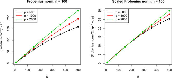
Convergence in Frobenius norm. Monte Carlo estimate of (Left) $E\Vert \widehat{\sum }-{\sum }^{\ast }{\Vert }_F^2/p$ and (Right) $E\Vert \widehat{\sum }-{\sum }^{\ast }{\Vert }_F^2/(p\log p)$ as a function of K, the bandwidth of Σ*

Figure 3.

Comparison of our procedure with simple and general weights.

5.1.2 Convergence rate dependence on n

To investigate the dependence on sample size, we vary n along an equally-spaced grid from 10 to 500, fixing K = 50 and taking, as before, p ∈ {500, 1000, 2000}. Simulating as before and taking, again $\lambda =2\sqrt{\log (p)/n}$, Figure 4 exhibits the 1/n dependence suggested by the bound in Corollary 2. In Section A.11 of the supplementary materials we observe the $1/\sqrt{n}$ behavior for operator norm in agreement with Theorem 9.

Figure 4.

(Left:) For large n, expected $E\Vert \widehat{\sum }-{\sum }^{\ast }{\Vert }_F^2/p$ is seen to decay like n⁻¹ as can be seen from −1 slope of log-log plot (gray lines are of slope −1). (Right:) Scaling this quantity by log p aligns the curves for large n. Both of these phenomena are suggested by Corollary 2.

5.1.3 Comparison to other banded estimators

In this section, we compare the performance of the following methods that perform banded covariance estimation: (i) <m>Hier Band:</m> our method with weights given in (2.6) and no eigenvalue constraint; (ii) <m>Simple Hier Band:</m> our method with weights given in (2.5) and no eigenvalue constraint; (iii) <m>GP Band:</m> group lasso without hierarchy (weighting scheme given in (2.4)) and no eigenvalue constraint; (iv) <m>Block Thresh:</m> Cai & Yuan (2012)’s block-thresholding approach (our implementation); (v) <m>BandChol:</m> Rothman et al. (2010)’s banding of the Cholesky factor approach via solving successive regression problems; (vi) <m>Banding:</m> Bickel & Levina (2008)’s T ∗ S estimator with T_jk = 1_{{|j−k|≤K}}.

Each method has a single tuning parameter that is varied to its best-case value. In the case of <m>Banding</m>, this makes it equivalent to an oracle-like procedure in which all non-signal elements are set to zero and all signal elements are left unshrunken.

While we focus on estimation error as a means of comparison, it should be noted that these methods could be evaluated in other ways as well. For example, <m>Banding</m> and <m>Block Thresh</m> frequently lead to estimators that are not positive semidefinite. This means that these covariance estimates cannot be directly used in other procedures requiring a covariance matrix (see, e.g., Section 5.2 for an example where not being positive definite would be problematic).

We simulate four scenarios for the basis of our comparison: (i) <m>MA(5):</m> with p = 200, n = 100. See Section 5.1.1 for description. (ii) <m>MA(80):</m> with p = 500, n = 100. See Section 5.1.1 for description. (iii) <m>CY:</m> A setting used in Cai & Yuan (2012) in which Σ^∗ is only approximately banded: ${\sum }_{ij}^{\ast }=0.6{|i-j|}^{-2}{U}_{ij}$, where U_ij = U_ji ~ Uniform(0, 1). We take p = 200, n = 100. (iv) <m>Increasing operator norm:</m> We produce a sequence of Σ^∗ having increasing operator norm. In particular, we take a block-diagonal matrix with p/K blocks of size K: Σ = I_p/K ⊗B_K; each block is $B_K=(0.8)1_K{1}_K^T+(0.2)I_K$; we take p = 1000, n = 100, and vary K between 20 and 400. We can make several observations from this comparison. We find that the hierarchical group lasso methods outperform the regular group lasso. This is to be expected since in our simulation scenarios, the true covariance matrix is banded (or approximately banded). As noted before, since we report the best performance of each method over all values of the tuning parameter, <m>Banding</m> is effectively an “oracle” method in that the banding is being performed exactly where it should be for <m>MA(5)</m>. So it is no surpise that this method does so well in this scenario. However, in the approximately banded scenario it suffers, likely because it does not do as well as methods that do shrink the nonzero values. We find that the <m>Block Thresh</m> does not perform very well in any of these scenarios (though Figure 5 does show it substantially improves on the sample covariance matrix). Finally, we find that the <m>BandChol</m> method performs well (although not shown here, we also observed that the related Nested Lasso method of Rothman et al. (2010) performs quite well).

Figure 5.

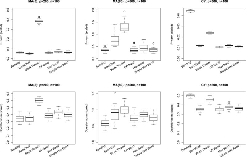
Comparison of methods in three settings in terms of (Top) squared Frobenius norm, relative to $\Vert S-{\sum }^{\ast }{\Vert }_F^2$ and (Bottom) operator norm relative to ‖S − Σ^∗‖_op.

Figure 6 shows the results for the third scenario, in which we consider a sequence of Σ^∗’s that are block diagonal with operator norm increasing linearly in K. Upon examination of the <m>Block Thresh</m> method’s estimates, we find that the reason this estimator peforms poorly in the regime of large K is that it sets all elements to zero that are sufficiently far from the main diagonal without regard to their observed size in S (this is referred to as step b in their paper). <m>Banding</m> performs very well in terms of operator norm, which makes sense since Σ^∗ is a banded matrix and so simple banding with the correct bandwidth is essentially an oracle procedure.

Figure 6.

Comparison of methods in terms of (Left) squared Frobenius norm and (Right) operator norm in a setting where ‖Σ^∗‖_op is increasing.

5.2 An application to discriminant analysis of phoneme data

In this section, we develop an application of our banded estimator. In general, one would expect any procedure that requires an estimate of the covariance matrix to benefit from convex banding when the true covariance matrix is banded (or approximately banded). Consider the classification setting in which we observe n i.i.d. pairs, (x_i, y_i), where x_i ∈ ℝ^p is a vector of predictors and y_i labels the class of the ith point. In quadratic discriminant analysis (QDA), one assumes that x_i|y_i = k ~ N_p (μ^∗(k), Σ^∗(k)). The QDA classification rule is to assign x ∈ ℝ^p to the class k maximizing $\widehat{\mathbb{P}}(y=k|\mathbf{x})$. Here $\widehat{\mathbb{P}}$ denotes the estimate of ℙ(y = k|x) given by replacing the parameters μ^∗(k), Σ^∗(k), and ℙ(y = k) with their maximum likelihood estimates.

To demonstrate the use of our covariance estimate in QDA, we consider a binary classification problem described in Hastie et al. (2009). The dataset consists of short sound recordings of male voices saying one of two similar sounding phonemes, and the goal is to build a classifier for automatic labeling of the sounds. The predictor vectors, x, are log-periodograms, representing the (log) intensity of the recordings across p = 256 frequencies. Because the predictors are naturally ordered, one might expect a regularized estimate of the within-class covariance matrix to be appropriate, and inspection of the sample covariance matrices (see Figure A.3 in Section A.12 of the supplementary materials) supports this. There are n₁ = 695 and n₂ = 1022 phonemes in the two classes. We randomly split the data into equal sized training and test sets. On the training set, five-fold cross validation is performed to select tuning parameters (λ₁, λ₂) and then the convex banding estimates, ${\widehat{\sum }}_{{\lambda }_1}^{(1)}$ and ${\widehat{\sum }}_{{\lambda }_2}^{(2)}$, are used in place of the sample covariances to form the basis of the prediction rule, $\widehat{\mathbb{P}}(y=k|\mathbf{x})$. The left panel of Figure 7 shows that QDA can be substantially improved by using a regularized estimate (and, in particular, that convex banding does quite well). Linear discriminant analysis (LDA) is like QDA but assumes a common covariance matrix between classes, Σ^∗(k) = Σ^∗, which is typically estimated as ${\mathbf{S}}_w=\frac{1}{n_1+n_2-2}[(n_1-1){\mathbf{S}}^{(1)}+(n_2-1){\mathbf{S}}^{(2)}]$, where ${\mathbf{S}}^{(k)}={(n_k-1)}^{-1}{\displaystyle {\sum }_{i=1}^{n_k}({\mathrm{x}}_i-{\overline{\mathrm{x}}}^{(k)}){({\mathrm{x}}_i-{\overline{\mathrm{x}}}^{(k)})}^T}$. The right panel of Figure 7 shows that LDA does better than the QDA methods, as expected in this regime of p and n (see, e.g., Cheng 2004) and can itself be improved by a regularized version of S_w, in which we replace S^(k) in the above expression with ${\widehat{\sum }}_{{\lambda }_k}^{(k)}$ (again, cross validation is performed to select the tuning parameters).

Figure 7.

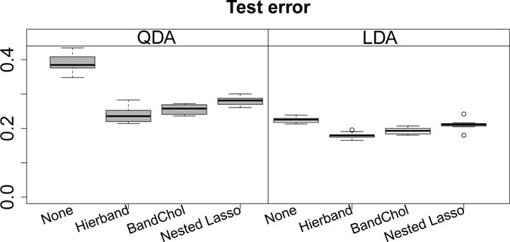
Test set misclassification error rates of discriminant analysis of phoneme data. For both QDA and LDA, using a regularized covariance matrix improves the misclassification error rate.

6 Conclusion

We have introduced a new kind of banding estimator of the covariance matrix that has strong practical and theoretical performance. Formulating our estimator through a convex optimization problem admits precise theoretical results and efficient computational algorithms. We prove that our estimator is minimax rate adaptive in Frobenius norm over the class of semi-banded matrices introduced in Section 4.2.1 and minimax rate adaptive in operator norm over the class of banded matrices, up to multiplicative logarithmic factors. Both classes of matrices over which optimality is established are allowed to have bandwidth growing with n, p or both. The construction of adaptive estimators over these classes, with established rate optimality is, to the best of our knowledge, new. Moreover, the proposed estimators recover the true bandwidth with high probability, for truly banded matrices, under minimal signal strength conditions. In contrast to existing estimators, our proposed estimator, which enjoys all the above theoretical properties, is guaranteed to be both exactly banded, and positive definite, with high probability. We also propose a version of the estimator, that is guaran teed to be positive definite in finite samples. Simulation studies show that the hierarchically banded estimator is a strong and fast competitor of the existing estimators. Through a data example, we demonstrate how our estimator can be effectively used to improve classification error of both quadratic and linear discriminant analysis. Indeed, we expect that many common statistical procedures that require a covariance matrix may be improved by using our estimator when the assumption of semi-bandedness is appropriate. An <m>R</m> (R Core Team 2013) package, named <m>hierband</m>, will be made available, implementing our estimator.

References

- Bach F, Jenatton R, Mairal J, Obozinski G. Structured sparsity through convex optimization. Statistical Science. 2012;27(4):450–468. [Google Scholar]
- Bickel PJ, Levina E. Regularized estimation of large covariance matrices. The Annals of Statistics. 2008:199–227. [Google Scholar]
- Bien J, Taylor J, Tibshirani R. A lasso for hierarchical interactions. The Annals of Statistics. 2013;41(3):1111–1141. doi: 10.1214/13-AOS1096. [DOI] [PMC free article] [PubMed] [Google Scholar]
- Bunea F, Xiao L. On the sample covariance matrix estimator of reduced ef fective rank population matrices, with applications to fpca. To appear in Bernoulli. 2014 arXiv:1212.5321. [Google Scholar]
- Cai TT, Yuan M. Adaptive covariance matrix estimation through block thresh-olding. The Annals of Statistics. 2012;40(4):2014–2042. [Google Scholar]
- Cai TT, Zhang CH, Zhou HH. Optimal rates of convergence for covariance matrix estimation. The Annals of Statistics. 2010;38(4):2118–2144. [Google Scholar]
- Cai TT, Zhou HH. Optimal rates of convergence for sparse covariance matrix estimation. The Annals of Statistics. 2012;40(5):2389–2420. [Google Scholar]
- Cheng Y. Asymptotic probabilities of misclassification of two discriminant functions in cases of high dimensional data. Statistics & Probability Letters. 2004;67(1):9–17. [Google Scholar]
- Dempster AP. Covariance selection. Biometrics. 1972;28(1):157–175. [Google Scholar]
- Hastie T, Tibshirani R, Friedman J. The Elements of Statistical Learning; Data Mining, Inference and Prediction. Second. Springer Verlag; New York: 2009. [Google Scholar]
- Jenatton R, Audibert J, Bach F. Structured variable selection with sparsity-inducing norms. The Journal of Machine Learning Research. 2011;12:2777–2824. [Google Scholar]
- Jenatton R, Mairal J, Obozinski G, Bach F. Proximal methods for sparse hierarchical dictionary learning. Proceedings of the International Conference on Machine Learning (ICML) 2010 [Google Scholar]
- R Core Team. R: A Language and Environment for Statistical Computing. R Foundation for Statistical Computing; Vienna, Austria: 2013. URL: http://www.R-project.org/ [Google Scholar]
- Radchenko P, James GM. Variable selection using adaptive nonlinear interaction structures in high dimensions. Journal of the American Statistical Association. 2010;105(492):1541–1553. [Google Scholar]
- Ravikumar P, Wainwright MJ, Raskutti G, Yu B, et al. High-dimensional covariance estimation by minimizing 1-penalized log-determinant divergence. Electronic Journal of Statistics. 2011;5:935–980. [Google Scholar]
- Rothman A, Levina E, Zhu J. A new approach to Cholesky-based covariance regularization in high dimensions. Biometrika. 2010;97(3):539. [Google Scholar]
- Tibshirani R. Regression shrinkage and selection via the lasso. J Royal Stat Soc B. 1996;58:267–288. [Google Scholar]
- Tseng P. Convergence of a block coordinate descent method for nondifferentiable minimization. Journal of optimization theory and applications. 2001;109(3):475–494. [Google Scholar]
- Xiao H, Wu WB, et al. Covariance matrix estimation for stationary time series. The Annals of Statistics. 2012;40(1):466–493. [Google Scholar]
- Xiao L, Bunea F. On the theoretic and practical merits of the banding estimator for large covariance matrices. arXiv preprint. 2014 arXiv:1402.0844. [Google Scholar]
- Yuan M, Lin Y. Model selection and estimation in regression with grouped variables. Journal of the Royal Statistical Society, Series B. 2006;68:49–67. [Google Scholar]
- Zhao P, Rocha G, Yu B. The composite absolute penalties family for grouped and hierarchical variable selection. The Annals of Statistics. 2009;37(6A):3468–3497. [Google Scholar]
Associated Data
This section collects any data citations, data availability statements, or supplementary materials included in this article.