

Abstract
Free energy calculations at finite temperature based on ab initio molecular dynamics (AIMD) simulations have become possible, but they are still highly computationally demanding. Besides, achieving simultaneously high accuracy of the calculated results and efficiency of the computational algorithm is still a challenge. In this work we describe an efficient algorithm to determine accurate free energies of solids in simulations using the recently proposed temperature-dependent effective potential method (TDEP). We provide a detailed analysis of numerical approximations employed in the TDEP algorithm. We show that for a model system considered in this work, hcp Fe, the obtained thermal equation of state at 2000 K is in excellent agreement with the results of standard calculations within the quasiharmonic approximation.
Introduction
Development of density functional theory (DFT), its implementation within efficient computational software packages in combination with rapid increase of computer power puts on the agenda a possibility of using simulations based on the most fundamental laws of quantum physics for solving important scientific challenges,1 as well as technologically relevant tasks. The simulations, named ab initio, are widely used in a variety of applications ranging from multidisciplinary research projects to accelerated knowledge-based materials design. However, standard DFT calculations are carried out at zero temperature, and this significantly reduces predictive power of the theory. Ab initio molecular dynamics (AIMD) allows one to overcome this limitation. Compared with classical molecular dynamics simulations, AIMD does not require any fitting parameters because the force fields are calculated from first principles. On the contrary, running AIMD simulations to obtain accurate free energies is always an extremely demanding problem in terms of required computational resources.
However, the free energy calculations give an important insight into the behavior of the system in the case of applied pressure and at finite temperature. The state-of-the-art approach is based on independent calculations of harmonic, quasiharmonic, and anharmonic contributions to the free energy.2,3 In dynamically stable systems, the anharmonic contribution to the free energy is relatively small. Unfortunately, there is no efficient way to compute it. Moreover, in systems with dynamical instabilities, the conventional technique fails completely. Therefore, the treatment of the anharmonic effects typically requires the use of additional techniques, such as thermodynamic integration.4 In this paper, we show how the recently developed temperature-dependent effective potential (TDEP) method5,6 can be applied to calculate the free energy, taking care of all the contributions simultaneously.
The TDEP employs AIMD, and therefore it is important to optimize the TDEP algorithm. Here we describe a computationally efficient scheme of executing TDEP. The theoretical background of TDEP has been presented earlier,5,6 and it has been applied with great success in numerous studies of lattice dynamics.7−13 Here we focus on the details of the computational algorithm. We demonstrate its performance in calculations of the equation of state (EOS) of hexagonal close-packed (hcp) iron at extreme conditions of ultrahigh pressure and temperature.
The choice of the model system is governed by high theoretical interest for the behavior of iron at Earth’s core conditions. There are substantial uncertainties of the experimentally, as well as theoretically, estimated values of the properties of Fe, e.g., its crystal structure, elasticity, thermal conductivity, and melting temperature.14−21 In addition, there are uncertainties between shock wave experiments22−24 and experiments carried out in laser-heated diamond anvil cells.25,26 In particular, it is extremely important to know the thermal and pressure-dependent behavior of elastic properties of iron at such conditions because it allows for better understanding of the seismological data obtained up to this point. The recent paper by Wang et al.(27) suggests that the treatment of seismological data heavily depends on the elastic model of Fe. Even though iron is one of the most theoretically studied materials, there are still a lot of questions to be answered, because most of the ab initio structural stability calculations and estimation of elastic constants have been done at 0 K.21,28−36 An ability to model the thermal equation of state of Fe theoretically is a necessary starting point to address the challenges specified above. We show that the equation of state of hcp iron at high pressures and high temperature, 2000 K, can be obtained accurately using TDEP. We compare our results with calculations done within quasiharmonic approximation carried out by Sha and Cohen.37 Therefore, the choice of temperature and pressure range is governed by a need to stay within the validity range of the quasiharmonic approximation, which is a standard theoretical method of investigating vibrational contributions to the Helmholtz free energy. Demonstrating the reliability of the results of a new method in a comparison with existing state-of-the-art tools has been recently mentioned as a necessary prerequisite to using the novel tool in solutions of more advanced tasks.1
Theory Behind the Method
Let us first outline the basics of the temperature-dependent effective potential method, focusing on the details, relevant to our presentation of the TDEP algorithm. The detailed description of the TDEP is available in refs (5) and (6).
Temperature-Dependent Effective Potential Method
To include vibrational effects, we introduce a temperature-dependent model Hamiltonian:
| 1 |
where ui and pi are the displacement
and momentum vectors of the atom i, and  (T) is the temperature-dependent
interatomic force constants matrix, which connects the displacement ui of atom i with
the resulting force fj acting
on atom j, at temperature T. For
a system consisting of total Na atoms,
in a harmonic approximation the forces and displacements are connected
via the force constants as follows:
(T) is the temperature-dependent
interatomic force constants matrix, which connects the displacement ui of atom i with
the resulting force fj acting
on atom j, at temperature T. For
a system consisting of total Na atoms,
in a harmonic approximation the forces and displacements are connected
via the force constants as follows:
 |
2 |
The basic idea of TDEP consists of
fitting the parameters U0 and  of the Hamiltonian in eq 1 to the results of AIMD
simulations at temperature T to give the best possible
harmonic approximation of the
lattice dynamics of a studied real (anharmonic) system. This is achieved
via a minimization of the difference in forces calculated from the
model Hamiltonian by eq 2 and real forces in the studied system.
of the Hamiltonian in eq 1 to the results of AIMD
simulations at temperature T to give the best possible
harmonic approximation of the
lattice dynamics of a studied real (anharmonic) system. This is achieved
via a minimization of the difference in forces calculated from the
model Hamiltonian by eq 2 and real forces in the studied system.
We note that it is possible to expand the right-hand side of eq 1 to include the third-order force constant term.38 These constants can be used to further improve the description of highly anharmonic systems and calculate important properties such as phonon lifetimes. In our case it was not necessary to include them because hcp Fe is weakly anharmonic for the conditions studied. The algorithm outlined in the next section can still be used with such higher-order model Hamiltonian.
Free Energy Calculations within the TDEP Method
Our task consists of calculation of the equation of state, that is, to determine pressure–volume relations. In the experiment, applied pressure plays the role of the input parameter, but for the simulation in the NVT ensemble, often employed in AIMD, the pressure is the outcome with the volume being the input parameter instead. Though it is possible to carry out simulations in the NPT ensemble, they are currently not well suited for use with the TDEP method because the underlying formalism assumes a constant volume when fitting results of the MD simulation to obtain the force-constant matrix in (2). In the case of an NVT-type simulation, the pressure is calculated from the free energy of the system in question:
| 3 |
where F is the Helmholtz free energy, V is the system volume, and P is the pressure. Therefore, to have an accurate pressure, we have to obtain an accurate Helmholtz free energy at several volumes to ensure accurate calculation of the derivative. The calculations at each volume require AIMD simulations, making the task numerically demanding. To minimize the number of AIMD runs is therefore beneficial for the efficiency of the TDEP algorithm. Below we show that it is possible to redistribute terms in calculations of F with TDEP in such a way as to ensure (nearly) linear volume dependence of the terms that require AIMD simulations, while nonlinear terms are determined from static calculations. Because of this, the accurate numerical calculations of volume derivatives for a wide range of pressures can be achieved with AIMD executed at just few volumes (five volumes in our case).
In the TDEP formalism,5,6 the Helmholtz free energy F consists of two terms, namely, vibrational contribution Fph and a ground-state energy U0 of a auxiliary model system, given by Hamiltonian in eq 1:
| 4 |
The vibrational contribution is obtained in the harmonic approximation39 via
| 5 |
where ℏ
is the reduced Planck’s
constant, kB is the Boltzmann constant,
ω is the phonon frequency, and g(ω) is
the phonon density of states, calculated in a conventional way but
with temperature-dependent force constant matrix  from eqs 1 and 2. We note in passing that,
in simulations that require variation of temperature, the interatomic
force constants can be interpolated as a function of temperature and
volume, as they often behave very smoothly in these parameters’
spaces, further increasing the efficiency of the algorithm.
from eqs 1 and 2. We note in passing that,
in simulations that require variation of temperature, the interatomic
force constants can be interpolated as a function of temperature and
volume, as they often behave very smoothly in these parameters’
spaces, further increasing the efficiency of the algorithm.
The ground-state energy of the model system U0 is determined in the following way:
| 6 |
where t is the simulation time, for which the averaging is carried out, UMD(t) is the temperature-dependent potential energy from AIMD simulation at time t, and α and β are Cartesian coordinates.
We reiterate that U0 is the ground-state energy of the auxiliary model system and, therefore, typically, differs from both converged potential energy of AIMD simulation and the DFT total energy calculated at 0 K.
Redistribution of Terms for an Efficient and Accurate Helmholtz Free Energy Calculations with the TDEP Method
In weakly anharmonic systems around equilibrium, Fph in eq 4 exhibits an almost linear volume dependence at fixed temperature,40 whereas the U0 term in (4) is a nonlinear function with respect to volume. To capitalize on this observation and to reduce the required amount of long AIMD simulations, we suggest a rearrangement of the terms in eq 4 in such a way that the nonlinearity is shifted to terms that can be calculated with static DFT calculations rather than with the tedious molecular dynamics simulations. Let us introduce an auxiliary function ΔU:
| 7 |
where Usupercellideal is the volume-dependent free energy of an “ideal” static supercell used in AIMD simulations. Note that the static calculations are carried out at the same temperature as AIMD, and the term includes the electronic entropy. Thus, it is “ideal” in a sense that all ions occupy their nondistorted ideal positions, with no displacement whatsoever. Next, we define Uuc as the volume-dependent free energy, which includes the potential energy and the electronic entropy terms at temperature T of a corresponding ideal unit cell corresponding to the supercell used in AIMD. In our case of Fe, this is the hcp unit cell.
In the case of perfect convergence of all the simulations parameters, Usupercellideal = K * Uuc, where K is an integer number, that accounts for the number of unit cells contained in the supercell. This is rarely the case though for any reasonbly sized supercells, because carrying out fully converged calculations turns out to be too resource-consuming. At this point it is important to note that the calculation of Uuc(V) can be carried out with high accuracy and at a dense set of volumes to describe accurately its nonlinear volume dependence, whereas the volume dependence of ΔU(V) often turns out to be nearly linear, similar to that of Fph(V). Therefore, one may use fewer AIMD simulations at different volumes to achieve the desired accuracy of the fitting for ΔU(V) as well as Fph(V). In particular, in our case of hcp Fe at temperature 2000 K, we carried out just five AIMD simulations. Finally, we obtain
| 8 |
The nonlinear behavior of F(V) is now predominantly concentrated in the volume dependence of the unit cell Uuc(V). In the case of our model system hcp Fe, the unit cell consists of two atoms and the volume dependence of Uuc(V) can be calculated with extremely high precision, because these calculations are computationally cheap.
For example, in our case of simulating hcp Fe at 2000 K, we use only five MD runs within the chosen pressure interval at the temperature in question to fit the nearly linear-dependent terms in (8). Once we perform all additional static calculations needed for the use of eq 8, including calculations of Uuc at 50 volumes, we would now effectively have 50 data points of the Helmholtz free energy F. Now it can be fitted and differentiated with high precision.
Computational Algorithm for the Temperature-Dependent Effective Potential Method
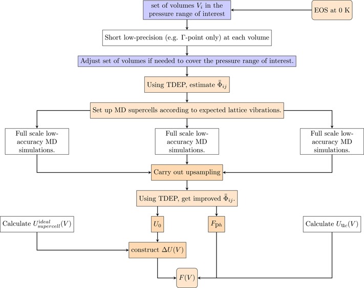
The flowchart of the algorithm for the calculation of pressure dependence of the free energy with TDEP method is shown in Figure 1. The full algorithm can be outlined as follows:
-
1.
Pick up the desired (minimal) number of volumes at which AIMD simulations will be carried out within the range of pressures of interest for the study. Note that the pressure at a finite temperature might differ from the 0 K equation of state value. Still, calculating P(V) at 0 K yields a good guess for the initial set of volumes {Vi} that can be used for molecular dynamics simulations.
-
2.
For each of the volumes in {Vi}, carry out a low-precision short MD simulation (e.g., with the Γ-point BZ integration scheme), still long enough for the system to to get a reasonable estimate of the interatomic force constants of the Hamiltonian (1) using the TDEP method. From our experience, with the hcp Fe, this usually takes up to 100–150 timesteps.
-
3.
Estimate the resulting pressures for each simulation. If the resulting pressures are not close enough to the initial points, adjust the initial set of volumes and repeat the low-precision simulations until the estimated AIMD pressures are indeed in the range of interest.
-
4.
Using the estimated interatomic force constants, prepare the supercells in a thermally excited state following the methodology of West and Estreicher.41 In connection with the TDEP method, the realization of this procedure has been described by Steneteg et al.42 These supercells can be used as multiple uncorrelated starting points to carry out highly parallel molecular dynamics simulation. Indeed, the so-constructed starting points are independent of each other and they correspond to physically relevant points of the simulated system phase space, virtually eliminating a need for the equilibration of the so-designed simulation cells. As a result, the AIMD simulations become highly parallel, allowing efficient execution of TDEP calculations by high-performance massively parallel supercomputers. However, even in a serial execution mode, the procedure described above greatly reduces the time needed to equilibrate the system.
-
5.
Carry out a longer converged low-precision simulation to obtain uncorrelated samples for the follow-up upsampling (see point 6 below). Because two consequent timesteps in molecular dynamics simulation are highly correlated, one in general needs to carry out a simulation with several orders of magnitude more timesteps than the number of samples needed for the upsampling, the static high-precision DFT calculations (dense BZ integration grid, higher cutoff energy).
-
6.
Carry out upsampling. By upsampling we mean that instead of using AIMD with fully converged parameters for the electronic structure calculations, one extracts uncorrelated samples from the low-accuracy AIMD and carries out highly accurate static electronic structure calculations for the samples.2 This can be done in parallel, because all such simulations are independent of each other. The force constants matrix components then can be estimated using these high-precision forces values according to (2). The TDEP vibrational contribution and ground-state energy then need to be calculated according to eqs 5 and 6, with UMD(t) term in (6) based on the high-precision calculation, and averaging needs to be done over the total amount of samples. The amount of the samples needed for the upsampling is determined by the desired accuracy of the simulated property and needs to be increased until the convergence is obtained. In our case we used stress tensor components and the total energy of the system as the target convergence variables.
-
7.
Using TDEP, obtain the force constants from high-precision data points. This allows one to obtain the phonon part Fph of the Helmholtz free energy as a function of volume as well as the values of the ground-state energy U0 of our model system U0. See eqs 5 and 6.
-
8.
Calculate ΔU and Uuc (eq 8) as a functions of volume V in the same range of volumes, with the highest possible precision (high density of BZ integration grid, high-energy cutoff).
-
9.
Combine the calculated dependencies to obtain the Helmholtz free energy F in the form of a smooth function of V. In our case the data set was dense enough to fit the dependence of F with respect to V with a polynomial of fourth order and in this way to obtain the analytical expression for the F(V) to be used in the calculation of the equation of state.
-
10.
Calculate the derivative of F(V) to obtain pressure as a function of volume (3), which yields the P(V) equation of state for the simulated system.
Figure 1.

Flowchart for Helmholtz free energy calculation algorithm with the TDEP method. The step labeled “Full scale low-accuracy MD simulations” can be done in parallel using different initial supercells.
Computational Details
This paper focuses on specifics of a typical calculation with TDEP in combination with projector augmented wave (PAW) method,43 as it is implemented in VASP.44−49 The molecular dynamics simulations were carried out in the Born–Oppenheimer approximation, which effectively means that the nuclei propagated via classical molecular dynamics and the electronic structure problem is solved with a fixed nuclear positions at that instance of time.50 The exchange–correlation energy term was treated within the generalized gradient approximation in the PBE form.51 In this work, the temperature in ab initio molecular dynamics simulations was controlled by the means of a Nose–Hoover thermostat.52
When studying hexagonal lattice, it is common to introduce a lattice parameters ratio between out-of-plane distance c and in-plane a, the so-called c/a ratio. For our model system, the hcp Fe, we used fixed c/a of 1.6. There is an ongoing discussion on the behavior of c/a at the Earth core conditions. There were reports on high c/a values up to 1.7 at the Earth core conditions,21,53 which later were corrected by molecular dynamics simulations.54,55 Experimentally, c/a of hcp Fe at room temperature and high pressure is known to be around 1.6.56 Recent experiments reported weak temperature dependence of the c/a ratio up to 2000 K57 in a range from 1.596 and 1.608, meaning that the temperature variations are comparable to experimental error. Using fixed c/a simplifies the calculations, allowing us to focus on the algorithm description.
All simulations were carried out on a 4 × 4 × 3 supercell of 96 atoms. For the molecular dynamics simulations, the following set of volumes per atom was chosen: {7.72928 Å3, 7.1706 Å3, 6.7648 Å3, 6.4394 Å3, 6.164 Å3}.
The low-accuracy AIMD simulations were carried out using computationally cheap PAW potential with 8 valence electrons with the default energy cutoff of 268 eV for this PAW potential. However, the reliability of the use of this PAW potential at high pressure was checked in comparison with those constructed for 14 and 16 valence electrons, as well as with the all-electron calculations, as will be discussed below. For the high-precision settings during the upsampling, we used a 3 × 3 × 3 Brillouin zone integration grid and the energy cutoff of 700 eV. To calculate the smooth dependency for Uuc, we took 50 equidistantly spaced volumes in the same range of volumes with cutoff energy of 700 eV and 31 × 31 × 31 integration grid generated by Monkhorst–Pack method.58
To interpolate the resulting volume dependency of Helmholtz free energy F(V), we used a fourth-order polynomial expression.
The accuracy of the PAW potentials used in our simulations was verified via comparison of the forces from VASP calculations with the forces computed using the result of full-potential linearized augmented plane wave (FPLAPW) all-electron calculation implemented in Wien2k.59 FPLAPW calculations were performed on a few atomic configurations extracted from AIMD run using VASP. The same number of Brillouin zone integration points was used in VASP and Wien2k: it was carried out with the Γ-point. The product of plane-wave cutoff and muffin-tin sphere radius was kept equal to 7, and the amount of electrons in valence band per atoms was kept constant regardless of VASP PAW potential and equal to 16.
Results and Discussion
Choice of PAW Potential
The PAW potentials library used in VASP is generated using the frozen core approximation, and therefore, calculations of forces should depend on its choice, especially for high-pressure calculations. The standard available PAW potentials of iron for VASP use 8, 14, or 16 valence electrons. It is reasonable to assume that one should include more electrons in the valence band as we go toward lower V/V0 values, where V0 is a system’s volume at zero external pressure. However, the computational cost increases nonlinearly with the increasing number of electrons. Therefore, we aim at achieving an intricate balance between the desired accuracy and complexity of the calculations performed.
It is important to note that the accuracy of PAW potentials is most often studied by converging scalar quantities, like total energies. However, for AIMD simulations, accurate forces are required. We are not aware of any published accuracy test on force calculations for Fe at extreme conditions. To find out which PAW potential is best suited for our task, the following test was carried out. For each of the Fe PAW potential available for VASP, we ran a short molecular dynamics simulation (400 time steps for equilibration of 1 fs each). Then few configurations of ionic positions from the subset of simulation were selected randomly, and calculations of forces were carried out. The resulting forces were then compared to the result of FPLAPW all-electron calculation implemented in Wien2k59 performed on the same atomic configurations. The result of the comparison is shown in Table 1 for the tested PAW potentials with varying amount of electrons in the valence band.
Table 1. Forces Comparison Test between PAW Potentials in VASP and FPLAPW All-Electron Calculation Carried out Using Wien2ka.
| sample | Zval | ρ(fr) | σ(fr) | ρ(fφ) | σ(fφ) | ρ(fθ) | σ(fθ) |
|---|---|---|---|---|---|---|---|
| 1 | 8 | 0.9742 | 0.3224 | 0.9934 | 0.1158 | 0.9994 | 0.0160 |
| 2 | 8 | 0.9969 | 0.2091 | 0.9884 | 0.1492 | 0.9947 | 0.0702 |
| 3 | 8 | 0.9985 | 0.3039 | 0.9903 | 0.1181 | 0.9947 | 0.0687 |
| 4 | 8 | 0.9956 | 0.2607 | 0.9899 | 0.1105 | 0.9964 | 0.0551 |
| 5 | 14 | 0.9891 | 0.1945 | 0.9873 | 0.1735 | 0.9898 | 0.0593 |
| 6 | 14 | 0.9911 | 0.2402 | 0.9899 | 0.1780 | 0.9902 | 0.0641 |
| 7 | 14 | 0.9898 | 0.3369 | 0.9806 | 0.2725 | 0.9934 | 0.0624 |
| 8 | 14 | 0.9903 | 0.4554 | 0.9868 | 0.1733 | 0.9925 | 0.0614 |
| 9 | 16 | 0.9709 | 0.3378 | 0.9961 | 0.1236 | 0.9906 | 0.0813 |
| 10 | 16 | 0.9900 | 0.1964 | 0.9920 | 0.1774 | 0.9977 | 0.0419 |
| 11 | 16 | 0.9952 | 0.2892 | 0.9927 | 0.1417 | 0.9967 | 0.0546 |
| 12 | 16 | 0.9984 | 0.1666 | 0.9910 | 0.1044 | 0.9965 | 0.0497 |
In Table 1, Zval denotes the amount of electrons in the valence band for the VASP PAW potential (for FPLAPW in Wien2k this value was kept constant and equal to 16); fr, fθ, and fφ are components of the forces in a spherical coordinate system;60 ρ is the correlation coefficient between the two sets of data, obtained in VASP and Wien2k calculations, respectively,
| 9 |
where μ(fVASP) and μ(fWien2k) represent the mean values of the forces averaged over the supercell,
| 10 |
and the standard deviation σ is defined as
| 11 |
N being a total number of ions in the supercell.
It is clear that there is no significant difference in the behavior of the forces in comparison among the tested PAW potentials; they all are as good as (or as bad as) the calculation performed by Wien2k. We therefore conclude that due to the nature of the simulations (long ab initio molecular dynamics runs), it is worth choosing the PAW-potential with the lowest amount of electrons in the valence band, because this allows for a faster calculation.
Helmholtz Free Energy Contributions
At this point let us come back to the contributions in the right-hand side of eq 8 and discuss how the proposed algorithm affects the Helmholtz free energy calculations with the TDEP method. The phonon contribution Fph is depicted in Figure 2, the auxiliary ΔU function defined in eq 7 is depicted in Figure 3, the ground-state total energy of the TDEP model Hamiltonian U0 is shown in Figure 4. Additionally, Figure 5 shows the nonlinear part of the ΔU expression, namely, the total energy of nondisplaced unit cell Uuc. The final F(V) for hcp Fe at 2000 K is shown in Figure 6. The gray crosses show the values from the initial low-precision MD simulations, and the red circles show results after the TDEP algorithm was applied as described in this paper. From Figure 6 one can see that our technique results in a much smoother dependence of F with respect to V than the initial low-precision simulation results. This smooth curve can be easily differentiated to obtain P(V) as defined in eq 3. In Figure 2 one can see that the vibrational contribution Fph(V) calculated from the initial low-precision simulations appears to behave almost linearly. However, for the case of U0 on Figure 4 one can see that the low-precision simulations (gray crosses) result in a kink at higher pressures, which then goes away after the upsampling technique is applied (red circles). Figure 3 depicts the dependence of ΔU with respect to volume. The data (red circles) in that figure are fitted with a linear function (black line), and then the resulting expression is used to obtain the final result for F(V), as expressed by eq 8.
Figure 2.
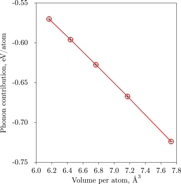
Vibrational contribution to Helmholtz Free energy of hcp Fe at 2000 K obtained with eq 5. Red circles show values that were obtained using the upsampling procedure. Initial results obtained with low-precision AIMD are shown as black crosses (in this particular case, the points are on nearly on top of each other). The points are connected with lines as a guide for the eyes.
Figure 3.

ΔU, eq 7, as a function of volume (red circles) The black line represents the linear fit: the deviation is in range from 1 to 5 meV/atom and is higher at lower volumes. The standard deviation is 4 meV.
Figure 4.

TDEP ground-state energy U0 of hcp Fe at 2000 K obtained with the method described in this paper compared to initial low-precision results. Red circles show values that were obtained using the upsampling scheme. Initial results from low-precision simulation AIMD are shown as gray crosses. The points are connected with lines as a guide for the eyes.
Figure 5.

Unit cell energy Uuc as a function of volume, calculated at electronic temperature 2000 K using high-precision settings and a dense set of volumes. This is the main nonlinear term in eq 7.
Figure 6.
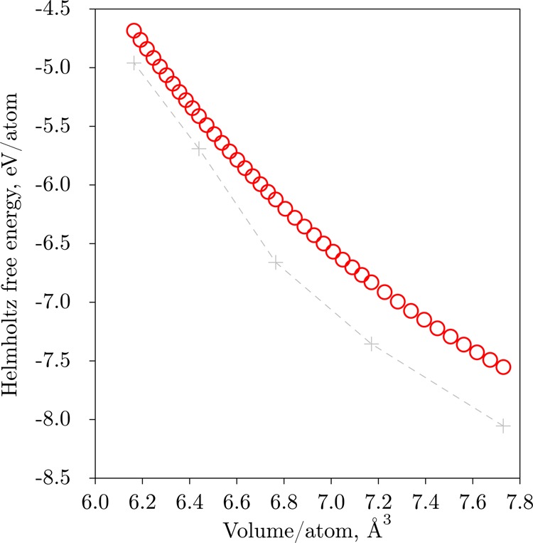
Helmholtz Free energy of hcp Fe at 2000 K obtained with the method described in this paper. Red circles show values that were obtained using high-precision molecular dynamics with enhanced scheme, outlined in this work. Initial results from low-precision simulation AIMD are shown as gray crosses. The points are connected with lines as a guide for the eyes.
Qualitatively, the different displayed behavior between the initial low-precision and final (upsampled) results is the illustration of the advantages of the proposed algorithm for calculations of free energy within TDEP method.
Equation of State of hcp Fe at 2000 K
To test the developed method, we investigate the EOS of hcp Fe at extreme conditions of T = 2000 K and P = 150–450 GPa, which contains the range of pressures relevant for the geophysical simulations with some leeway. These conditions are within the validity range of the state-of-the-art quasiharmonic approximation (QHA), and therefore, the results of TDEP calculations can be compared directly to those of the quasiharmonic calculations. This is possible due to the temperature dependence of the force constants of hcp Fe is negligible in the validity range of QHA.
The resulting EOS is shown in Figure 7 (red circles), alongside data from QHA calculation by Sha and Cohen37 (blue line), fitted using Vinet equation of state.61 For the Sha and Cohen data, the Vinet equation of state gives an equilibrium volume of 10.081 Å. For our calculation the equilibrium volume was found to be 10.283 Å. Note, however, that our data set was limited to the high-pressure range where the applicability of GGA-DFT calculations is well established. At lower-pressure many-electron effects play an important role in simulations of the ground-state properties of hcp Fe.62,63 Therefore, here we excluded it from the consideration.
Figure 7.

Pressure in hcp Fe as a function of V/V0 at T = 2000 K. Blue line: data from quasiharmonic calculation by Sha and Cohen37 Red data points: this work.
Very good agreement between two curves in the chosen pressure range shows the reliability of our algorithm, as well as the TDEP method.
Conclusion
We present a detailed description of the algorithm of highly efficient free energy calculations using the temperature-dependent effective potential method. We illustrate the reliability and efficiency of the method by calculating the equation of state of hcp Fe at 2000 K.
The results are in excellent agreement with state-of-the-art
calculations
within the quasiharmonic approximation. Moreover, the TDEP method
is designed to be used for simulations of strongly anharmonic solids,
because the fit to AIMD takes into account the temperature-dependence
of both the force constants matrix  and potential
energy landscape. This, in
particular, will allow us to carry out simulations of Fe and Fe-based
alloys at the Earth’s core conditions.
and potential
energy landscape. This, in
particular, will allow us to carry out simulations of Fe and Fe-based
alloys at the Earth’s core conditions.
Acknowledgments
The data used in Figure 7 was based on results of QHA calculation from the paper by X. Sha and R. E. Cohen37 and was kindly provided by the authors. We are grateful for the support provided by the Swedish Foundation for Strategic Research (SSF) program SRL Grant No. 10-0026, the Swedish Research Council (VR) grants No. 2015-04391, No. 2014-4750, and No. 637-2013-7296, the Swedish Government Strategic Research Area in Materials Science on Functional Materials at Linköping University (Faculty Grant SFO-Mat-LiU No. 2009 00971), as well as by the Ministry of Education and Science of the Russian Federation (Grant No. 14.Y26.31.0005). Calculations were performed utilizing supercomputer resources supplied by the Swedish National Infrastructure for Computing (SNIC) at the PDC and NSC centers (PRACE-2IP project FP7 RI-283493), and at supercomputer cluster Cherry at NUST ”MISIS”.
The authors declare no competing financial interest.
References
- Lejaeghere K.; Bihlmayer G.; Björkman T.; Blaha P.; Blügel S.; Blum V.; Caliste D.; Castelli I. E.; Clark S. J.; Dal Corso A.; et al. Reproducibility in Density Functional Theory Calculations of Solids. Science 2016, 351, aad3000–aad3000. 10.1126/science.aad3000. [DOI] [PubMed] [Google Scholar]
- Grabowski B.; Ismer L.; Hickel T.; Neugebauer J. Ab initio up to the Melting Point: Anharmonicity and Vacancies in Aluminum. Phys. Rev. B: Condens. Matter Mater. Phys. 2009, 79, 134106. 10.1103/PhysRevB.79.134106. [DOI] [Google Scholar]
- Alfe D.; Price G. D.; Gillan M. J. Thermodynamics of Hexagonal-Close-Packed Iron under Earth’s Core Conditions. Phys. Rev. B: Condens. Matter Mater. Phys. 2001, 64, 18. 10.1103/PhysRevB.64.045123. [DOI] [Google Scholar]
- Jorge M.; Garrido N. M.; Queimada A. J.; Economou I. G.; Macedo E. A. Effect of the Integration Method on the Accuracy and Computational Efficiency of Free Energy Calculations Using Thermodynamic Integration. J. Chem. Theory Comput. 2010, 6, 1018–1027. 10.1021/ct900661c.20467461 [DOI] [Google Scholar]
- Hellman O.; Abrikosov I. A.; Simak S. I. Lattice Dynamics of Anharmonic Solids from First Principles. Phys. Rev. B: Condens. Matter Mater. Phys. 2011, 84, 180301. 10.1103/PhysRevB.84.180301. [DOI] [Google Scholar]
- Hellman O.; Steneteg P.; Abrikosov I. A.; Simak S. I. Temperature Dependent Effective Potential Method for Accurate Free Energy Calculations of Solids. Phys. Rev. B: Condens. Matter Mater. Phys. 2013, 87, 104111. 10.1103/PhysRevB.87.104111. [DOI] [Google Scholar]
- Chen Y.; Ai X.; Marianetti C. A. First-Principles Approach to Nonlinear Lattice Dynamics: Anomalous Spectra in PbTe. Phys. Rev. Lett. 2014, 113, 105501. 10.1103/PhysRevLett.113.105501. [DOI] [PubMed] [Google Scholar]
- Errea I.; Calandra M.; Mauri F. First-Principles Theory of Anharmonicity and the Inverse Isotope Effect in Superconducting Palladium-Hydride Compounds. Phys. Rev. Lett. 2013, 111, 177002. 10.1103/PhysRevLett.111.177002. [DOI] [PubMed] [Google Scholar]
- Monserrat B.; Drummond N. D.; Pickard C. J.; Needs R. J. Electron-Phonon Coupling and the Metallization of Solid Helium at Terapascal Pressures. Phys. Rev. Lett. 2014, 112, 055504. 10.1103/PhysRevLett.112.055504. [DOI] [PubMed] [Google Scholar]
- Zhou F.; Nielson W.; Xia Y.; Ozolinš V. Lattice Anharmonicity and Thermal Conductivity from Compressive Sensing of First-Principles Calculations. Phys. Rev. Lett. 2014, 113, 185501. 10.1103/PhysRevLett.113.185501. [DOI] [PubMed] [Google Scholar]
- Zhang D.-B.; Sun T.; Wentzcovitch R. M. Phonon Quasiparticles and Anharmonic Free Energy in Complex Systems. Phys. Rev. Lett. 2014, 112, 058501. 10.1103/PhysRevLett.112.058501. [DOI] [PubMed] [Google Scholar]
- Romero A. H.; Gross E. K. U.; Verstraete M. J.; Hellman O. Thermal Conductivity in PbTe from First Principles. Phys. Rev. B: Condens. Matter Mater. Phys. 2015, 91, 214310. 10.1103/PhysRevB.91.214310. [DOI] [Google Scholar]
- Shulumba N.; Hellman O.; Rogström L.; Raza Z.; Tasnádi F.; Abrikosov I. A.; Odén M. Temperature-Dependent Elastic Properties of Ti1-xAlxN Alloys. Appl. Phys. Lett. 2015, 107, 231901. 10.1063/1.4936896. [DOI] [Google Scholar]
- Kübler J. Metastable Magnetic Ground-State of HCP-Fe. Solid State Commun. 1989, 72, 631–633. 10.1016/0038-1098(89)90662-5. [DOI] [Google Scholar]
- Belonoshko A. B. Equation of State for ε-Iron at High Pressures and Temperatures. Condens. Matter Phys. 2010, 13, 23605. 10.5488/CMP.13.23605. [DOI] [Google Scholar]
- Buffett B. a.; Wenk H. R. Texturing of the Earth’s Inner Core by Maxwell Stresses. Nature 2001, 413, 60–63. 10.1038/35092543. [DOI] [PubMed] [Google Scholar]
- Cohen R. E.; Mukherjee S. Non-collinear Magnetism in Iron at High Pressures. Phys. Earth Planet. Inter. 2004, 143-144, 445–453. 10.1016/j.pepi.2004.02.002. [DOI] [Google Scholar]
- Gilder S. Magnetic Properties of Hexagonal Closed-Packed Iron Deduced from Direct Observations in a Diamond Anvil Cell. Science 1998, 279, 72–74. 10.1126/science.279.5347.72. [DOI] [PubMed] [Google Scholar]
- Lin J.-f.; Heinz D. L.; Campbell A. J. Iron-Silicon Alloy in Earth’s Core?. Science 2002, 295, 313–315. 10.1126/science.1066932. [DOI] [PubMed] [Google Scholar]
- Merkel S. Raman Spectroscopy of Iron to 152 Gigapascals: Implications for Earth’s Inner Core. Science 2000, 288, 1626–1629. 10.1126/science.288.5471.1626. [DOI] [PubMed] [Google Scholar]
- Steinle-Neumann G.; Stixrude L.; Cohen R. E.; Gülseren O. Elasticity of Iron at the Temperature of the Earth’s Inner Core. Nature 2001, 413, 57–60. 10.1038/35092536. [DOI] [PubMed] [Google Scholar]
- Brown J. M.; McQueen R. G. Phase Transitions, Grüneisen Parameter, and Elasticity for Shocked Iron between 77 and 400 GPa. J. Geophys. Res. 1986, 91, 7485. 10.1029/JB091iB07p07485. [DOI] [Google Scholar]
- Nguyen J. H.; Holmes N. C. Melting of Iron at the Physical Conditions of the Earth’s Core. Nature 2004, 427, 339–42. 10.1038/nature02248. [DOI] [PubMed] [Google Scholar]
- Yoo C.; Holmes N.; Ross M.; Webb D.; Pike C. Shock Temperatures and Melting of Iron at Earth Core Conditions. Phys. Rev. Lett. 1993, 70, 3931–3934. 10.1103/PhysRevLett.70.3931. [DOI] [PubMed] [Google Scholar]
- Shen G.; Mao H.-k.; Hemley R. J.; Duffy T. S.; Rivers M. L. Melting and Crystal Structure of Iron at High Pressures and Temperatures. Geophys. Res. Lett. 1998, 25, 373–376. 10.1029/97GL03776. [DOI] [Google Scholar]
- Boehler R. Temperatures in the Earth’s Core from Melting-point Measurements of Iron at High Static Pressures. Nature 1993, 363, 534–536. 10.1038/363534a0. [DOI] [Google Scholar]
- Wang T.; Song X.; Xia H. H. Equatorial Anisotropy in the Inner Part of Earth’s Inner Core from Autocorrelation of Earthquake Coda. Nat. Geosci. 2015, 8, 224–227. 10.1038/ngeo2354. [DOI] [Google Scholar]
- Stixrude L.; Cohen R. E. High-Pressure Elasticity of Iron and Anisotropy of Earth’s Inner Core. Science 1995, 267, 1972–1975. 10.1126/science.267.5206.1972. [DOI] [PubMed] [Google Scholar]
- Söderlind J.; Moriarty P.; Wills J. M. First-principles Theory of Iron up to Earth-Core Pressures: Structural, Vibrational, and Elastic Properties. Phys. Rev. B: Condens. Matter Mater. Phys. 1996, 53, 14063–14072. 10.1103/PhysRevB.53.14063. [DOI] [PubMed] [Google Scholar]
- Qiu S.; Marcus P. Elasticity of HCP Nonmagnetic Fe under Pressure. Phys. Rev. B: Condens. Matter Mater. Phys. 2003, 68, 054103. 10.1103/PhysRevB.68.054103. [DOI] [Google Scholar]
- Vočadlo L.; Alfè D.; Gillan M.; Price G. The Properties of Iron under Core Conditions from First Principles Calculations. Phys. Earth Planet. Inter. 2003, 140, 101–125. 10.1016/j.pepi.2003.08.001. [DOI] [Google Scholar]
- Asker C.; Vitos L.; Abrikosov I. A. Elastic Constants and Anisotropy in FeNi Alloys at High Pressures from First-principles Calculations. Phys. Rev. B: Condens. Matter Mater. Phys. 2009, 79, 214112. 10.1103/PhysRevB.79.214112. [DOI] [Google Scholar]
- Kádas K.; Vitos L.; Ahuja R. Elastic Properties of Iron-rich HCP Fe-Mg Alloys up to Earth’s Core Pressures. Earth Planet. Sci. Lett. 2008, 271, 221–225. 10.1016/j.epsl.2008.04.003. [DOI] [Google Scholar]
- Vočadlo L.; Dobson D. P.; Wood I. G. Ab initio Calculations of the Elasticity of HCP-Fe as a Function of Temperature at Inner-core Pressure. Earth Planet. Sci. Lett. 2009, 288, 534–538. 10.1016/j.epsl.2009.10.015. [DOI] [Google Scholar]
- Steinle-Neumann G.; Cohen R. E. Comment on ’On the Importance of the Free Energy for Elasticity under Pressure’. J. Phys.: Condens. Matter 2004, 16, 8783–8786. 10.1088/0953-8984/16/47/028. [DOI] [Google Scholar]
- Bercegeay C.; Bernard S. First-principles Equations of State and Elastic Properties of Seven Metals. Phys. Rev. B: Condens. Matter Mater. Phys. 2005, 72, 214101. 10.1103/PhysRevB.72.214101. [DOI] [Google Scholar]
- Sha X.; Cohen R. E. First-principles Thermal Equation of State and Thermoelasticity of HCP Fe at High Pressures. Phys. Rev. B: Condens. Matter Mater. Phys. 2010, 81, 094105. 10.1103/PhysRevB.81.094105. [DOI] [Google Scholar]
- Hellman O.; Abrikosov I. A. Temperature-dependent effective third-order interatomic force constants from first principles. Phys. Rev. B: Condens. Matter Mater. Phys. 2013, 88, 144301. 10.1103/PhysRevB.88.144301. [DOI] [Google Scholar]
- Van de Walle A.; Ceder G. The Effect of Lattice Vibrations on Substitutional Alloy Thermodynamics. Rev. Mod. Phys. 2002, 74, 11–45. 10.1103/RevModPhys.74.11. [DOI] [Google Scholar]
- Wallace Duanne C.Thermodynamics of Crystals; Dover Publications: New York, 1998. [Google Scholar]
- West D.; Estreicher S. K. First-principles Calculations of Vibrational Lifetimes and Decay Channels: Hydrogen-related Modes in Si. Phys. Rev. Lett. 2006, 96, 115504. 10.1103/PhysRevLett.96.115504. [DOI] [PubMed] [Google Scholar]
- Steneteg P.; Hellman O.; Vekilova O. Yu.; Shulumba N.; Tasnádi F.; Abrikosov I. A. Temperature Dependence of TiN Elastic Constants from ab initio Molecular Dynamics Simulations. Phys. Rev. B: Condens. Matter Mater. Phys. 2013, 87, 094114. 10.1103/PhysRevB.87.094114. [DOI] [Google Scholar]
- Blöchl P. E. Projector Augmented-Wave Method. Phys. Rev. B: Condens. Matter Mater. Phys. 1994, 50, 17953. 10.1103/PhysRevB.50.17953. [DOI] [PubMed] [Google Scholar]
- VASP Group, Computational Matherials Physics. Vienna ab-initio Simulation Package, version 5.2; University of Vienna. [Google Scholar]
- Kresse G.; Furthmüller J. Efficiency of ab-initio Total Energy Calculations for Metals and Semiconductors using a Plane-Wave Basis Set. Comput. Mater. Sci. 1996, 6, 15–50. 10.1016/0927-0256(96)00008-0. [DOI] [PubMed] [Google Scholar]
- Kresse G.; Joubert D. From Ultrasoft Pseudopotentials to the Projector Augmented-Wave Method. Phys. Rev. B: Condens. Matter Mater. Phys. 1999, 59, 1758. 10.1103/PhysRevB.59.1758. [DOI] [Google Scholar]
- Kresse G.; Hafner J. Ab initio Molecular Dynamics for Liquid Metals. Phys. Rev. B: Condens. Matter Mater. Phys. 1993, 47, 558–561. 10.1103/PhysRevB.47.558. [DOI] [PubMed] [Google Scholar]
- Kresse G.; Hafner J. Ab initio Molecular-Dynamics Simulation of the Liquid-Metal–Amorphous-Semiconductor Transition in Germanium. Phys. Rev. B: Condens. Matter Mater. Phys. 1994, 49, 14251–14269. 10.1103/PhysRevB.49.14251. [DOI] [PubMed] [Google Scholar]
- Kresse G.; Furthmüller J. Efficient Iterative Schemes for ab initio Total-Energy Calculations using a plane-wave basis set. Phys. Rev. B: Condens. Matter Mater. Phys. 1996, 54, 11169–11186. 10.1103/PhysRevB.54.11169. [DOI] [PubMed] [Google Scholar]
- Marx D.; Hutter J.. Ab initio Molecular Dynamics: Theory and implementation; John-von-Neumann-Inst. for Computing: Julich, 2000. [Google Scholar]
- Perdew J. P.; Burke K.; Ernzerhof M. Generalized Gradient Approximation Made Simple. Phys. Rev. Lett. 1996, 77, 3865–3868. 10.1103/PhysRevLett.77.3865. [DOI] [PubMed] [Google Scholar]
- Nose S.; Nosé S.; Nosé S. A Unified Formulation of the Constant Temperature Molecular Dynamics Methods. J. Chem. Phys. 1984, 81, 511–519. 10.1063/1.447334. [DOI] [Google Scholar]
- Wasserman E.; Stixrude L.; Cohen R. E. Thermal Properties of Iron at High Pressures and Temperatures. Phys. Rev. B: Condens. Matter Mater. Phys. 1996, 53, 8296–8309. 10.1103/PhysRevB.53.8296. [DOI] [PubMed] [Google Scholar]
- Alf D.; Gillan M. J.; Price G. D. The Melting Curve of Iron at the Pressures of the Earth’s Core from ab initio Calculations. Nature 1999, 401, 462–464. 10.1038/46758. [DOI] [Google Scholar]
- Alfè D.; Kresse G.; Gillan M. J. Structure and Dynamics of Liquid Iron under Earth’s Core Conditions. Phys. Rev. B: Condens. Matter Mater. Phys. 2000, 61, 132–142. 10.1103/PhysRevB.61.132. [DOI] [Google Scholar]
- Takahashi T.; Bassett W. A. High-Pressure Polymorph of Iron. Science 1964, 145, 483–486. 10.1126/science.145.3631.483. [DOI] [PubMed] [Google Scholar]
- Ma Y.; Somayazulu M.; Shen G.; Mao H.-k.; Shu J.; Hemley R. J. In situ X-ray Diffraction Studies of Iron to Earth-Core Conditions. Phys. Earth Planet. Inter. 2004, 143–144, 455–467. 10.1016/j.pepi.2003.06.005. [DOI] [Google Scholar]
- Monkhorst H. J.; Pack J. D. Special Points for Brillouin-Zone Integrations. Phys. Rev. B 1976, 13, 5188–5192. 10.1103/PhysRevB.13.5188. [DOI] [Google Scholar]
- Blaha P.; Schwarz K.; Madsen G. K. H.; Kvasnicka D.; Luitz J.. WIEN2K, An Augmented Plane Wave Plus Local Orbitals Program for Calculating Crystal Properties; Techn. Universität Wien: Vienna, Austria, 2001. [Google Scholar]
- Given Cartesian components Fx, Fy, and Fz, spherical
components can be obtained using
 , Fθ =
cos–1(Fz/Fr) and Fφ = tan–1(Fy/Fx)
, Fθ =
cos–1(Fz/Fr) and Fφ = tan–1(Fy/Fx) - Vinet P.; Ferrante J.; Rose J. H.; Smith J. R. Compressibility of Solids. J. Geophys. Res. 1987, 92, 9319. 10.1029/JB092iB09p09319. [DOI] [Google Scholar]
- Glazyrin K.; Pourovskii L. V.; Dubrovinsky L.; Narygina O.; McCammon C.; Hewener B.; Schünemann V.; Wolny J.; Muffler K.; Chumakov A. I.; et al. Importance of Correlation Effects in HCP Iron Revealed by a Pressure-Induced Electronic Topological Transition. Phys. Rev. Lett. 2013, 110, 117206. 10.1103/PhysRevLett.110.117206. [DOI] [PubMed] [Google Scholar]
- Pourovskii L. V.; Mravlje J.; Ferrero M.; Parcollet O.; Abrikosov I. A. Impact of Electronic Correlations on the Equation of State and Transport in ε-Fe. Phys. Rev. B: Condens. Matter Mater. Phys. 2014, 90, 155120. 10.1103/PhysRevB.90.155120. [DOI] [Google Scholar]