. 2016 Dec 7;5:e20515. doi: 10.7554/eLife.20515

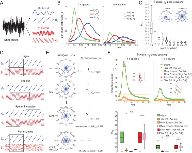
Figure 2. Detection of spurious n:m phase-locking in white-noise signals due to inappropriate surrogate-based statistical testing.

(A) Example white-noise signal (black) along with its theta- (blue) and gamma- (red) filtered components. The corresponding instantaneous phases are also shown. (B) n:m phase-locking levels for 1- (left) and 10 s (right) epochs, computed for noise filtered at theta (θ; 4–12 Hz) and at three gamma bands: slow gamma (γS; 30–50 Hz), middle gamma (γM; 50–90 Hz) and fast gamma (γF; 90–150 Hz). Notice Rn:m peaks in each case. (C) Boxplot distributions of θ−γS R1:5 values for different epoch lengths (n = 2100 simulations per epoch length). The inset shows representative Δφnm distributions for 0.3- and 100 s epochs. (D) Overview of surrogate techniques. See text for details. (E) Top panels show representative Δφnm distributions for single surrogate runs (Time Shift; 10 runs of 1 s epochs), along with the corresponding Rn:m values. The bottom panel shows the pooled Δφnm distribution; the Rn:m of the pooled distribution is lower than the Rn:m of single runs (compare with values for 1- and 10 s epochs in panel C). (F) Top, n:m phase-locking levels computed for 1- (left) or 10 s (right) epochs using either the Original or five surrogate methods (insets are a zoomed view of Rn:m peaks). Bottom, R1:5 values for white noise filtered at θ and γS. Original Rn:m values are not different from Rn:m values obtained from single surrogate runs of Random Permutation and Time Shift procedures. Less conservative surrogate techniques provide lower Rn:m values and lead to the spurious detection of θ−γS phase-phase coupling in white noise. *p<0.01, n = 2100 per distribution, one-way ANOVA with Bonferroni post-hoc test.

DOI: http://dx.doi.org/10.7554/eLife.20515.005

Figure 2.

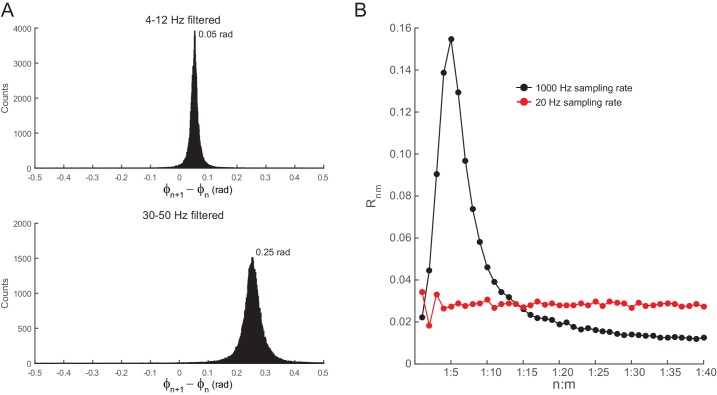
Figure 2—figure supplement 1. Filtering induces quasi-linear phase shifts in white-noise signals.

Figure 2—figure supplement 1.

(A) Distribution of the phase difference between two consecutive samples for white noise band-pass filtered at theta (4–12 Hz, top) and slow gamma (30–50 Hz, bottom). Epoch length = 100 s; sampling rate = 1000 Hz (dt = 0.001 s). Notice that the top histogram peaks at ~0.05, which corresponds to 2*3.14*8*0.001 (i.e., 2*π*fc*dt, where fc is the center frequency), and the bottom histogram peaks at ~0.25 =2*3.14*40*0.001. (B) Rn:m curves computed for theta- and slow gamma-filtered white-noise signals. The black curve was obtained using continuous 1 s long time series sampled at 1000 Hz. The red curve was obtained by also analyzing 1000 data points, but which were subsampled at 20 Hz (subsampling was performed after filtering). Notice Rn:m peak at n:m = 1:5 only for the former case. See also Figure 5—figure supplement 7 for similar results in hippocampal LFPs.
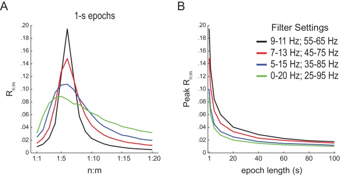
Figure 2—figure supplement 2. Filter bandwidth influences n:m phase-locking levels in white-noise signals.

Figure 2—figure supplement 2.

(A) Mean Rn:m curves computed for 1 s long white-noise signals filtered into different bands (same color labels as in B; n = 2100). Notice that the narrower the filter bandwidth, the higher the Rn:m peak. (B) Mean Rn:m peak values for different filter bandwidths and epoch lengths (n = 2100 simulations per filter setting and epoch length).
Figure 2—figure supplement 3. Uniform p-value distributions upon multiple testing of Original Rn:m values against Single Run Rn:m surrogates.

Figure 2—figure supplement 3.

The histograms show the distribution of p-values (bin width = 0.02) for 10000 t-tests of Original Rn:m vs Single Run surrogate values (n = 30 samples per group; epoch length = 1 s). The red dashed line marks p=0.05. The p-value distributions do not statistically differ from the uniform distribution (Kolmogorov-Smirnov test).