TACO produces robust multi-sample transcriptome assemblies from RNA-seq

Abstract

Accurate transcript structure and abundance inference from RNA-Seq data is foundational for molecular discovery. Here we present TACO, a computational method to reconstruct a consensus transcriptome from multiple RNA-Seq datasets. TACO employs novel change-point detection to demarcate transcript start and end sites, leading to dramatically improved reconstruction accuracy compared to other tools in its class. The tool is available at http://tacorna.github.io and can be readily incorporated into RNA-Seq analysis workflows.

High-throughput RNA sequencing (RNA-Seq) has enabled a deep understanding of the transcriptome^1–3. While efforts to annotate high fidelity gene models by manual and automated systems have relied primarily on low-throughput sequencing methods^4–6, several studies using RNA-Seq have described an expansive transcriptome, suggesting that reference gene catalogs are far from complete^3,7,8. This annotation gap has been widened further by the rapid sequencing of thousands of high quality RNA-Seq datasets by consortia such as TCGA⁹, ICGC¹⁰, and GTEX¹¹. Limitations of current reference annotation projects necessitate development of computational transcriptome assembly methods to utilize these large-scale RNA-Seq datasets for transcript discovery⁵.

Transcriptome reconstruction for single-sample experiments remains an active area of investigation. Although current reconstruction methods achieve high accuracy at the nucleotide or splice junction level, studies have shown that they do not reliably predict the splicing patterns of full-length transcripts¹². Moreover, single-sample transcriptome reconstruction has limited utility for the downstream analyses of transcriptional dynamics across many samples. To address this issue, a consensus transcriptome from multiple input datasets must be constructed, which can be done by merging individual transcriptome reconstructions in a hierarchical fashion. We term this procedure “meta-assembly”.

Current software for meta-assembly include the Cuffmerge utility within the Cufflinks package¹³ and a merge mode within the StringTie software (hereafter denoted ‘StringTie-merge’)¹⁴. We demonstrate that the performance of both Cuffmerge and StringTie-merge deteriorates as the number of input datasets increases, yielding myriad incorrectly predicted transcript structures with intron retentions, aberrantly long 3′ and 5′ ends, and read-through transcripts that concatenate multiple neighboring genes on the same strand. These errors may originate from contamination of the input libraries with incompletely processed RNA or genomic DNA^8,15, or be propagated from genome-guided assembly. To remain scalable, meta-assembly methodology must be designed to mitigate these sources of error.

Here we present a new meta-assembly method, TACO (Transcriptome Assemblies Combined into One), as a robust solution for leveraging the vast RNA-Seq data landscape for transcript structure prediction. To prepare data for TACO, sequence reads are aligned to a reference genome by a spliced alignment tool. Then, genome-guided transcript assembly is performed which serve as input to TACO (Figure 1). As a pure meta-assembler TACO remains agnostic to the alignment and assembly strategy used, and therefore can be readily incorporated into existing RNA-Seq analysis protocols such as the Tuxedo suite¹⁶ (see Supplementary Note, “Integration with other tools”). The software, written in Python and C, and its documentation can be obtained at http://tacorna.github.io. Runtime and memory usage statistics can be found in the Supplementary Note.

Figure 1.

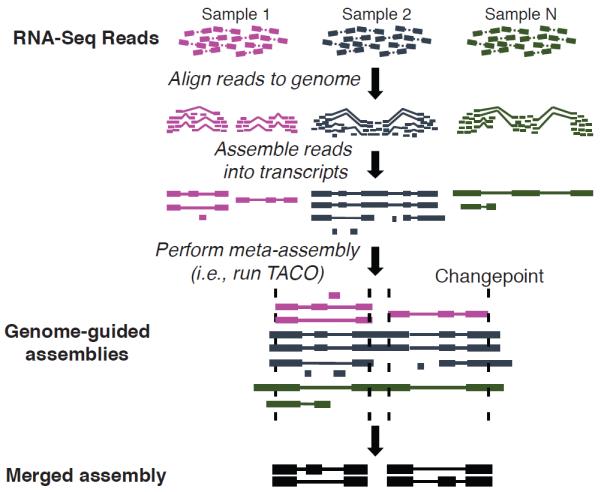
Schematic detailing the transcriptome meta-assembly workflow for TACO. Reads are initially aligned to the genome. Ab initio assembly is then performed, generating a transcriptome assembly for each input sample. These transcriptome assemblies are then merged into a meta-assembly using the TACO tool, which leverages change point detection and a dynamic programming algorithm to generate robust transcript isoforms from the underlying network of splicing patterns.

Building on existing transcriptome assembly methods, TACO approaches meta-assembly by modeling alternatively spliced genes using directed acyclic graphs, or splice graphs, built from the input transcripts (Supplementary Figure 1a and Methods). To harness the splicing pattern information present in the input transcripts, TACO constructs path graphs wherein each node corresponds to a sequence of consecutive splice junctions (Supplementary Figure 1b). TACO then applies dynamic programming to enumerate the set of isoforms with highest abundance. To mitigate the deleterious effects of incorrectly assembled input transcripts, TACO employs change point detection via binary segmentation to identify points of significant change of expression in the basewise transcript abundance landscape (Supplementary Figure 2). As evidenced by the performance tests detailed below, change point detection effectively breaks apart read-through transcripts and accurately delineates transcript start and end sites.

To assess the performance of TACO compared to other tools, we initially computed the precision, recall (i.e. sensitivity), and F-measure (harmonic mean of precision and recall) at the nucleotide, splice junction, and transcript splicing pattern (i.e. isoform) level while varying the number of input transcriptomes. We used RNA-seq data from the CCLE¹⁷ and used GENCODE v24 as a reference standard. TACO outperformed Cuffmerge and StringTie-merge in its ability to predict bases covered, splice junctions, and splicing patterns for runs with more 10 samples (Figure 2a and Supplementary Tables 1,2). The performance of Cuffmerge and StringTie-merge decreased as the number of samples increased, whereas TACO was robust to sample size. The most prominent advantage of TACO was its ability to identify correct splicing patterns, which is the most challenging goal of transcriptome assembly^12,14. Predicting correct isoforms is essential for downstream analysis, as abundance estimation applied to incorrectly assembled transcripts will likely be inaccurate. TACO achieved splicing pattern precision of approximately 30%, compared to about 5% for each of the other tools (Figure 2a, and Supplementary Table 3). Of note, the reported splicing pattern precision of individual sample transcriptome reconstruction tools is around 30%^12,14, suggesting that even when merging 500 samples, TACO displays little loss of accuracy.

Figure 2.

Assessment of TACO performance. a. Performance metrics for TACO, Cuffmerge, and Stringtie when merging different numbers of input assemblies. Recall (i.e., sensitivity), precision and the F-measure for all three tools were assessed for splicing patterns, splice junctions, and bases. Points represent the mean statistic across the 20 runs, error bars represent the 95% confidence interval. (Data to make this panel can be found in Supplementary Table 3) b,c. Precision-recall plots (left) and bar plots depicting the average precision (right) depicting performance for the three tools merging 55 CCLE breast cancer cell lines (a) at 50 different isoform fraction cutoffs ranging from 0.001-0.999, and (b) for the highest expressed transcripts in the meta-assemblies. Points represent statistics for the top N transcripts, with N ranging from 500-30,000. (Data to make panels b and c can be found in Supplementary Tables 4 and 6, respectively).

All three merging tools offer a key parameter, termed the “isoform fraction cutoff”, for filtering out minor isoforms based on their abundance relative to the major isoform. Adjusting this parameter results in a trade-off between precision and recall. Thus, by modulating this parameter we assessed performance the tools’ full range of precision and recall (Figure 2b, Supplementary Figure 3 and Supplementary Tables 1,4). TACO outperformed Cuffmerge and StringTie-merge across the spectrum of isoform fraction cutoffs, achieving an average precision (a statistic that serves as a surrogate “area under the curve” for precision-recall plots) of 0.53, 0.78, and 0.21 for bases covered, splice junctions, and splicing patterns, respectively, compared to 0.33, 0.75, and 0.06 for Cuffmerge and 0.41, 0.75, and 0.09 for StringTie-merge. Most prominent was TACO’s ability to reconstruct correct transcript splicing patterns with high precision (>50% for high isoform fraction cutoffs).

It is important to note that the selection of reference standard can heavily impact precision metrics, introducing potential biases depending on the nature of the reference selected. In addition to GENCODE, we also tested performance using long-read RNA-seq data as a reference standard, and the superior performance of TACO was consistent in these additional analyses (Supplementary Figure 4, Supplementary Table 5, and Supplementary Note, “Long-read RNA-seq as reference standard”).

We assessed how well the meta-assembly tools correctly prioritized transcripts that are highly expressed. Meta-assemblies using all three tools were generated, and transcript abundance from these assembled transcripts was quantified. We then measured each tool’s precision, recall, and F-measure on subsets of the top N most highly abundant transcripts, varying N from 500 to 30,000. TACO possessed a striking ability to predict the nucleotides, splice junctions, and splicing patterns of highly expressed transcripts, achieving an average precision of 0.45, 0.59, and 0.17, respectively, compared to 0.35, 0.49, 0.01 for Cuffmerge and 0.41, 0.54, and 0.03 for StringTie. Notably, TACO attained a splicing pattern precision of 76.8% for the top 5,000 most highly abundant transcripts, dramatically better than the 30% and 16.2% precision of StringTie-merge and Cuffmerge, respectively (Figure 2c, Supplementary Figure 5, and Supplementary Table 6).

In order to directly assess the efficacy of change point detection, we quantified the fraction of read-through genes produced by each tool (Supplementary Figure 6). At low isoform fraction cutoffs, ~10% and ~7.5% of the genes produced by StringTie-merge and Cuffmerge, respectively, contained multiple unique GENCODE genes (i.e., “read-throughs”), while only ~2.5% of TACO transcripts were read-throughs. This finding supports the effectiveness of change point detection in detecting transcription start and end sites. Reduction of read-through transcription is of potential benefit to downstream analyses, as read counting is particularly susceptible to the deleterious effects of read-through transcription, especially if the underlying genes encompassed by the read-through are highly discrepant in expression value. It is important to note, however, that some of this read-through transcription may be real transcriptional events (see Supplementary Note, “Read-through transcription” for further discussion).

As evidenced by the performance assessment above, TACO retains robust accuracy even when processing a large number of input datasets, producing higher-fidelity transcripts with read-throughs and spurious isoforms compared to Cuffmerge and StringTie-merge. We observed a representative example in the 3p21 genomic locus, which harbors three genes in close proximity on the negative strand (Figure 3). Although gene-dense regions are particularly challenging for meta-assembly, the change point detection and other algorithmic advances of TACO enable it to cleanly disambiguate all three genes, whereas Cuffmerge and StringTie-merge produce dozens of spurious isoforms, many of which are read-throughs. This problem is present when merging 50 samples and is exacerbated as the number of merged samples rises to 500 (Figure 3). Other examples are detailed in the Supplementary Note (“Examples”).

Figure 3.

Examples of TACO performance. The 3p21 genomic locus is depicted. Assembly of the genes SLC26A6, CELSR3, and NCKIPSD are shown for 50, 100, and 500 samples merged. The assembly produced by Cuffmerge is shown in blue, Stringtie in orange, and TACO in green. The Refseq reference annotation is shown above in red.

While extraordinary efforts of sequencing consortia have made thousands of high quality RNA-Seq datasets from diverse tissue types and disease states available to the scientific community, RNA-Seq continues to be an underutilized source of evidence for expanding reference transcript catalogs. The lack of a robust computational method to accurately coalesce large numbers of input datasets into a consensus transcriptome has been a major impediment to the use of RNA-Seq for this purpose. Given its accuracy and scalability, TACO has potential to facilitate progress in this area, and we expect that its adoption will help unravel the complexity of the transcriptome.

Online Methods

Genome-guided assembly

FASTQ files were obtained from DBGap (accession number phs000178) using the Cancer Genomics Hub (https://cghub.ucsc.edu). Reads were aligned to human genome version GRCh38/hg38 using STAR¹⁸ version 2.4.2 with the following parameters: --alignSJDBoverhangMin 3, --alignIntronMin 20, --alignSJoverhangMin 8, --alignMatesGapMax 1000000, --alignIntronMax 1000000, --scoreGenomicLengthLog2scale 0, --outSAMmode NoQS --outFilterType BySJout. Cufflinks¹³ (version 2.2.1) and StringTie¹⁴ (version 1.2.2) were utilized to produce transcriptome assemblies from the BAM alignments generated by STAR as detailed above.

Meta-assembly

Performance of Cuffmerge¹³ (version 2.2.1), StringTie-merge (version 1.2.2), and TACO were tested. Cuffmerge was run using default parameters except for the isoform fraction, “--min-isoform-fraction”, which was adjusted according to the appropriate analyses. StringTie was run with the analogous parameter (“-f”) for isoform fraction cutoff. For all analyses unless otherwise indicated, StringTie was run with the “-T” and “-F” parameters set to zero and TACO was run with the --filter-min-expr set to zero. These parameters filter the input transcripts using a provided expression cutoff. While StringTie-merge and TACO provide an option to filter input assemblies by expression level, Cufflinks does not provide this option, and so all analyses reported above were done with the expression filter option turned off for these tools. Comparing the performance of StringTie-merge and TACO run with a 1 FPKM (the StringTie-merge default) filtration of input transcripts did not reveal substantial differences in the tools’ performance. StringTie-merge did display an increase in performance at the base level, but TACO remained a superior tool for all metrics (base, splice junctions, splicing patterns) (Supplementary Figure 7).

Performance assessment

The performance of all meta-assemblies were assessed using the “gffcompare” utility version 0.9.5 (https://ccb.jhu.edu/software/stringtie/gff.shtml). All meta-assemblies were compared to GENCODE version 24 (level 1 protein-coding genes). Only poly-exonic transcripts were utilized in performance assessment (“-M” and “-N” gffcompare flags), and precision-correction was performed by only utilizing test transcripts overlapping reference (“-Q” flag in gffcompare). The average precision metric was utilized as a surrogate measure of the AUC for the precision / recall curve¹⁹ and was calculated as follows:

$$\sum _{k=1}^{N}P\left(k\right)\Delta r\left(k\right)$$

where N is the number of points samples, P(k) is the precision at point k, and Δr is the change in recall that occurs between point k-1 and k.

Sample size performance assessment

Performance of all three meta-assembly tools was measured at varying numbers of input assemblies. Twenty batches of different sizes ranging from 1 to 500 (Supplementary Table 2) were selected randomly from the 935 CCLE samples (Supplementary Table 1). All three tools were run using their default setting for the isoform fraction cutoff parameter (i.e., 0.05 for TACO, 0.05 for Cuffmerge, 0.01 for StringTie-merge).

Isoform fraction cutoff assessment

Cuffmerge, StringTie, and TACO were tested at varying ranges of isoform fraction cutoffs as described above. Meta-assembly was performed on the 55 breast cancer cell lines in the CCLE. To test the full range of performance for all tools the following isoform fraction cutoffs were used: 0.001, 0.00115139, 0.0013257, 0.0015264, 0.00175748, 0.00202354, 0.00232989, 0.00268261, 0.00308873, 0.00355633, 0.00409472, 0.00471462, 0.00542837, 0.00625017, 0.00719638, 0.00828584, 0.00954024, 0.01098453, 0.01264748, 0.01456218, 0.01676675, 0.01930507, 0.02222767, 0.02559271, 0.02946719, 0.03392823, 0.03906463, 0.04497862, 0.05178793, 0.05962811, 0.06865521, 0.07904892, 0.09101613, 0.10479506, 0.12065998, 0.1389267, 0.15995881, 0.18417497, 0.21205722, 0.24416056, 0.28112402, 0.32368339, 0.37268581, 0.42910671, 0.49406917, 0.5688663, 0.65498696, 0.75414543, 0.86831549, and 0.999.

Comparison to tissue PacBio long-read sequencing

Long-read PacBio RNA sequencing data was used as a comprehensive reference standard for meta-assembly performance assessment. Consensus split mapped molecules (CSMMs) for aligned PacBio reads from the Sharon et al. study²⁰ were obtained from http://stanford.edu/~htilgner/2013_NBT_paper/pacBio.index.html in GFF format. All GFF attributes arising from the same PacBio read were given a common transcript ID for conversion to GTF format to be utilized in reference statistics. Additonally, the gffread utility (part of the Cufflinks suite)¹³ was used to collapse overlapping CSMMs. Of the 20 tissue and organ types represented in the Sharon et al. study, 17 were present in the GTEX dataset. Three samples from each tissue type were selected at random, and fastq files for these samples were downloaded from dbGAP (phs000424). RNA-seq data was aligned as described above and Cufflinks was used to obtain transcriptome assemblies to be used as input for meta-assembly. Assessment of performance for the meta-assemblies was performed as described above using the gffcompare utility.

Comparison to brain long-read sequencing

CSMMs from long-read SLR-RNA-seq of multiple brain samples was used as an additional comprehensive reference standard. CSMMs from the Tilgner et al. study²¹ were obtained from http://stanford.edu/~htilgner/2014_humanMouseBrain_SLR_RNA_Seq/index_SLRseq.html in GFF format and converted to GTF format as described above. Fifty benign brain RNA-seq samples from GTEX were selected at random, and fastq files for these samples were downloaded from dbGAP (phs000424). RNA-seq data was aligned as described above and Cufflinks was used to obtain transcriptome assemblies to be used as input for meta-assembly. Assessment of performance for the meta-assemblies was performed as described above using the gffcompare utility.

Performance of highest expressed transcripts

In order to assess the performance of Cuffmerge, StringTie, and TACO, for the highest expressed transcripts, transcript abundance was estimated for the meta-assemblies produced from the merging of the 55 breast cancer CCLE samples using an isoform fraction cutoff of 0.05. The Kallisto RNA-seq isoform abundance estimation tool²² was used to calculate isoform abundance for all transcripts in the meta-assemblies produced by the three tools. Expression across the 55 samples was calculated as the sum of the TPM values reported by Kallisto for each transcript across all samples. The highest 100, 500, 1000, 1500, 2000, 3000, 5000, 7000, 10000, 12000, 15000, 18000, 20000, 22000, 25000, 27000, and 30000 transcripts were utilized to test performance of the tools.

Assessment of performance varying change point parameters

Performance of TACO was assessed by comparing to the GENCODE protein-coding genes as described above at different values for the change point p-value cutoff and the change point fold-change cutoff. The following p-value cutoffs were tested: 1, 0.5, 0.25, 0.1, 0.05, 0.01, 1e-3, 1e-4, 1e-5, 1e-6, 1e-7. The following fold-change cutoffs used: 1, 0.95, 0.9, 0.85, 0.7, 0.6, 0.5, 0.35, 0.25, 0.125, 0.0625, 0.03125.

Visualization of meta-assemblies

Examples of the meta-assembly performance were visualized using IGV²³. For the chromosome 3p21 locus the samples from run “0” (Supplementary Table 2) were utilized for batch sizes of 50, 100, 500. For all other loci, run “0” was used for a batch size of 100.

Overview of TACO meta-assembly approach

We developed TACO as a software package written in Python and C. The software adapts and builds upon methods that were developed previously by our bioinformatics group for the purposes of meta-assembly, and utilized for the MiTranscriptome project³. TACO accepts as input a set GTF files containing transcripts assembled from individual libraries. Transcripts can be filtered based on length in base pairs (--min-transfrag-length), with the TACO default set to filtering transcripts less than 200bp in length. TACO aggregates and sorts the input GTF files, and then parses the aggregated set of transcripts into independent loci with non-overlapping genomic coordinates. Within each locus, TACO reassigns unstranded mono-exonic transcripts to either the positive or negative strand whenever there is unambiguous supporting evidence of strandedness from the other transcripts in the locus. Transcripts on the positive and negative strand are then processed independently. TACO then clusters sets of overlapping transcripts on the same strand into splice graphs. Nodes in the splice graph comprise contiguous transcribed regions not interrupted by splicing. Once nodes are identified, the summed expression profile across each node is utilized to perform change point detection. For each change point identified, a new edge is created to the source or sink node, representing a potential transcript start or end site. Details of the various components of the TACO algorithm are found below. For further details, the TACO source code can be found at http://tacorna.github.io.

Details of TACO algorithm

Major Steps

1. Aggregate: Prior to meta-assembly, the input GTF files are merged and transcripts are sorted by chromosome and position. Filters for transcript length (--filter_min_length) and expression (--filter_min_expr) are applied.

2. Locus Identification: Transcripts in merged GTF file are partitioned into loci, where a locus is defined as a collection of input transcripts with overlapping genomic coordinates. Groups of transcripts from independent loci are then assembled in parallel.

3. Strand Imputation: TACO attempts to impute the strand for any unstranded transcripts included in the input data. See below for further details.

4. Determine Locus Expression: Stranded basewise expression of each locus is the summed expression from the input transcripts for each base determined by the individual transcriptome assembler utilized to generate the input transcriptome. Of note, TACO is compatible with any expression unit (as long as that unit is consistent for all samples used) and the unit of expression can be specified with the --gtf-expr-attr flag.

5. Build Splice Graphs: Transcripts within each locus are partitioned into splice graphs. A splice graph is a directed acyclic graph representing the stranded transcribed genomic regions of the input transcripts. See below for further details.

6. Change Point Detection: Change points are identified within each node in the splice graph (see definition below). Binary segmentation is used to recursively identify multiple points of change meeting significance criteria in each node’s expression profile. Upon identification of all change points in each node of a splice graph, the splice graph is updated with new connections to the source and/or sink. See below for further details.

7. Build Path Graph: A specialized graph structure called the path graph is derived from the splice graph. The path graph retains structural information from the input transcripts and encapsulates splicing pattern information into the graph. See below for further details.

8. Predict Isoforms: The path graph is iteratively traversed using a dynamic programming approach, yielding the most highly expressed isoforms in the gene. Users may specify how exhaustively the algorithm predicts isoforms using the --isoform-frac and/or --max-isoforms command line options.

9. Report output

Step Details

Strand Imputation

Unstranded transcript assemblies may arise from RNA-Seq data if the underlying reads are unstranded and the transcript is monoexonic. TACO attempts to impute the strand of each unstranded transcript using the following steps:

For each unstranded transcript T:

• If all stranded transcripts overlapping T are on the positive strand, then assign T to the positive strand

• If all stranded transcripts overlapping T are on the negative strand, then assign T to the negative strand

• If there are transcripts overlapping T on both the positive and negative strands, then the strand of T is deemed ambiguous and is not imputed

• If no stranded transcripts overlap T, then the strand of T is deemed ambiguous and is not imputed.

• By default, transcripts with ambiguous strand are not assembled unless the --assemble-unstranded option is enabled.

Splice Graph

TACO partitions the input transcripts within a locus by strand, and builds splice graphs from sets of overlapping transcripts within the locus. A splice graph is a directed acyclic graph representing the stranded transcribed genomic regions and splice junctions of the input transcripts.

Properties:

• Node: a contiguous exonic genomic interval with no internal splice donors or acceptors in the input transcripts

• Edge: connects nodes x and y if an input transcript contains x and y consecutively

• Expression: The expression of each node is determined by summing the expression of input transcripts that contain the node.

Creation:

1. Define Nodes:

   • ○
     To define nodes, we first iterate through the input transcripts and define the set of node boundaries. Nodes are bounded by splice donor/acceptor sites and transcriptional start/stop sites (e.g. sites where the summed expression of the input transcripts changes from zero to nonzero).
2. Define Edges:

   • ○
     After defining the set nodes in the splice graph, we iterate through the input transcripts in a second pass. For each transcript, we map its exons across node boundaries, thus representing the transcript as a sequence of nodes. We then add the edges inferred by this sequence to the set of all edges in the splice graph.

Change Point Detection

Change point detection is performed at the level of each node within a splice graph. Using the basewise expression for each node, recursive binary segmentation²⁴ of the change point detection algorithm is performed until potential change points fail to meet significance criteria. Once change points are detected for all nodes in a splice graph, the splice graph is updated to account for the new connections to the source and sink.

Definitions:

• Expression vector: the input for the change point detection algorithm. Initially, the expression vector is the number of bases of the entire splice graph node, whose values are the basewise expression of that node. In subsequent recursive iterations of the algorithm, the expression vector represents the basewise expression of the node segment being tested, whose boundaries are defined by previously identified change points.

• Mean squared error (MSE):

  $$\mathit{MSE}\left(m\right)=\sum _{i=1}^m{(X_i-{\overline{X}}_1)}^2+\sum _{i=m+1}^l{(X_i-{\overline{X}}_2)}^2$$

  • ○
    Where X is the expression vector being tested, m is the index of point being tested in the expression vector, X_i is the expression at index i of the expression vector, $\overline{X1}$ is the mean expression for bases 0 to m in the expression vector, l is the length of X, and $\overline{X2}$ is the mean expression for bases m + 1 to l
• Significance criteria for potential change points:

  • ○
    Mann-Whitney U (MWU) test must meet defined p-value threshold (--change-point-pvalue). The MWU compares the expression values only at points of change on either side of a potential change point.

    • ▪
      E.g., if the expression on either side of the potential change point are X₁ = [15, 15, 15, 15, 15, 14, 14, 14, 13, 13, 12, 12, 10] and X₂ = [10, 10, 10, 9, 9, 8, 8, 8, 8, 7, 7, 4, 4, 2, 2, 2, 3, 2, 2], the MWU will compare only the values where expression values changed X’₁ = [15, 14, 13, 12, 10] and X’₂ = [10, 9, 8, 7, 4, 2, 3, 2]
  • ○
    Fold-change comparing the mean expression on either side of the change point must meet a defined threshold (--change-point-fold-change).
  • ○
    Default settings for change point p-value and fold-change were determined by testing the performance of TACO at varying p-values and fold-changes (Supplementary Figure 8).

Algorithm:

For a given expression vector X:

• If the length of X < 20, do not perform change point detection

• Identify the base/index within X with the minimum MSE as a potential change point, PC.

• Test whether PC meets significance criteria

• If PC meets criteria:

  • ○
    Append point of change, C, to list of change points for a given node
  • ○
    Utilizing the expression on either side of C as a new expression vector to be fed back into the change point detection algorithm, recursively test for other change points (a.k.a, binary segmentation)

    • ▪
      As change points are often gradual and sloping, in order to prevent calling multiple change points along one slope, when a change point is identified, all bases on the same slope as the identified change point are removed from the expression vector used for future binary segmentation iterations

• If PC does not meet significance criteria, stop change point detection binary segmentation

Path Graph

After detecting change points in a splice graph, TACO builds a new graph structure called a path graph to encapsulate sequences of consecutive splice junctions. The data structure of the path graph is reminiscent of the De Bruijn graph model used for de novo assembly.

Properties:

• Node: a sequence of k nodes from the splice graph that appears in at least one input transcript. We subsequently refer to nodes in the path graph as “subpaths”.

• Edge: connects subpaths x and y if the last k-1 nodes in subpath x are equal to the first k-1 nodes in subpath y.

• Expression: the expression at each node equals the summed expression of all of the input transcripts that contain the node

• Source: subpaths originating at a transcriptional start site are connected to a common source node

• Sink: subpaths terminating at a transcriptional stop site are connected to a common sink node

Algorithm:

Creation of a path graph with subpaths of length k:

• For each input transcript T:

  • ○
    Define the sequence of splice graph nodes represented by T as NT
  • ○
    If the length of NT is less than k:

    • ▪
      If the first node of NT is a transcriptional start site and the last node of NT is a transcriptional stop site:

      • Add NT to the path graph as a single node with connections to the source and sink regardless of the length of NT or the value of k.
    • ▪
      Else:

      • Append NT to a list of short transcripts, to be dealt with later
  • ○
    Else:

    • ▪
      Add nodes NT[0..k], NT[1..k+1], NT[2..k+2], etc. to the path graph, with edges connecting consecutive nodes.
• Determine and remove unreachable nodes from the path graph:

  • ○
    If a node in the path graph is unreachable from either the source node or the sink node, remove it from the path graph
• Attempt to rescue short input transcripts

  • ○
    For each short input transcript ST (length of the sequences of nodes NT less than k):

    • ▪
      Determine all the nodes in the path graph that contain ST

      • This is done by first creating a suffix array index of all of the nodes in the path graph and then aligning the sequence ST to this index. Further details are available in the online source code.
    • ▪
      Allocate the expression of T to all matching nodes proportionally using the relative expression of each matching node.
• Extend transcripts that do not begin at a start site and end at a stop site:

  • ○
    If the first node of NT is not a transcriptional start site:

    • ▪
      Allocate the expression of T to all predecessor nodes of NT in a weighted fashion (see below). This is implemented using breadth first search starting at NT[0], traversing the graph in reverse until all possible paths to the source node are visited.
  • ○
    If the last node if NT is not a transcriptional stop site:

    • ▪
      Allocate the expression of T to all successor nodes of NT in a weighted fashion (see below). This is implemented using breadth first search starting at NT[−1], traversing the graph in the forward direction until all possible paths to the sink node are visited.
  • ○
    Expression is allocated to neighbor nodes (either predecessor or successor nodes depending on whether NT is being extended from its start site or stop site, respectively) in a weighted fashion, by using the fractional expression levels of all neighbor nodes. For example, if NT[0] with an expression level of 12 is being extended upstream to two possible neighbor (e.g. predecessor) nodes NA and NB with expression levels of 30 and 60, respectively, NA and NB will be allocated 4 and 8 expression units, respectively.
  • This procedure ensures that the summed expression at the source node equals the summed expression at the sink node.

Choice of k for creating the Path Graph

The choice of k for path graph construction poses an interesting tradeoff. As k decreases, the chances of assembling transcripts that do not represent the input data increases. In this case, even if input transcript predictions are incorrect the algorithm could still assemble correctly by utilizing expression information. By contrast, as k increases, the assembled transcripts will be increasingly constrained to precisely match paths in the input transcripts, and less dependent upon expression information in the input data. Optimal performance could theoretically be achieved by selecting a k that balances this tradeoff²⁵. Intuitively, the number of nodes in a path graph could be used as a surrogate measure for graph complexity. With more nodes (i.e., more subpaths) comes an increase in the potential diversity within the graph from which transcript isoforms are generated. Therefore, we select a value of k by maximizing the number of nodes in the ensuing path graph (efficient selection of the k yielding the maximum numbers of nodes is done using a bisection algorithm implementation). In practice, we observed that for most problems, plotting the value of k versus the number of nodes in the path graph follows a gaussian distribution, wherein there is a k_opt that results in a maximum of potential subpaths to traverse when generating transcript isoforms.

Predict Isoforms

Isoforms are predicted using a dynamic programming algorithm that traverses the nodes of path graph to find the most highly expressed isoform in the following steps:

• 1Predict isoform, I, and its expression, EXPR_I, that represents the most highly expressed path in the current path graph via dynamic programming.

a. The first isoform identified is designated I_max, with expression, EXPR_max. The absolute expression value at which to stop predicting additional isoforms is determined by multiplying EXPR_max by the value of the command line parameter --isoform-frac.

• 2Subtract EXPR_I from all of the nodes contained within I
• 3Repeat steps 1-2 to predict isoforms I and their expression values EXPR_I, terminating when EXPR_I is less than EXPR_max × isoform-frac

The dynamic programming algorithm is implemented as follows:

• For each node i in the path graph, initialize the following state variables:

  • ○
    Let min_expr[i] equal 0.0
  • ○
    Let prev[i] equal NULL
• For each node i in the path graph, ordered by topological sort:

  • ○
    For each successor node j of i:

    • ▪
      If (prev[j] is NULL) or min(min_expr[i], expr[j]) > min_expr[j]:

      • Let min_expr[j] equal min(min_expr[i], expr[j])
      • Let prev[j] equal i

A traceback loop then reconstructs the highest expression isoform by starting at the SINK node and prepending nodes in the prev vector until reaching the SOURCE.

Data Availability

Transcriptome assemblies and all references used as for this manuscript can be found at tacorna.github.io. TACO source code can also be found there.

References

- 1.Djebali S, et al. Landscape of transcription in human cells. Nature. 2012;489:101–8. doi: 10.1038/nature11233. [DOI] [PMC free article] [PubMed] [Google Scholar]
- 2.Mercer TR, et al. Targeted RNA sequencing reveals the deep complexity of the human transcriptome. Nat. Biotechnol. 2011;30:99–104. doi: 10.1038/nbt.2024. [DOI] [PMC free article] [PubMed] [Google Scholar]
- 3.Iyer MK, et al. The landscape of long noncoding RNAs in the human transcriptome. Nat Genet. 2015;47:199–208. doi: 10.1038/ng.3192. [DOI] [PMC free article] [PubMed] [Google Scholar]
- 4.Harrow J, et al. GENCODE: The reference human genome annotation for the ENCODE project. Genome Res. 2012;22:1760–1774. doi: 10.1101/gr.135350.111. [DOI] [PMC free article] [PubMed] [Google Scholar]
- 5.Pruitt KD, et al. RefSeq: An update on mammalian reference sequences. Nucleic Acids Res. 2014;42:756–763. doi: 10.1093/nar/gkt1114. [DOI] [PMC free article] [PubMed] [Google Scholar]
- 6.Cunningham F, et al. Ensembl 2015. Nucleic Acids Res. 2015;43:D662–D669. doi: 10.1093/nar/gku1010. [DOI] [PMC free article] [PubMed] [Google Scholar]
- 7.Cabili MN, et al. Integrative annotation of human large intergenic noncoding RNAs reveals global properties and specific subclasses. Genes Dev. 2011;25:1915–27. doi: 10.1101/gad.17446611. [DOI] [PMC free article] [PubMed] [Google Scholar]
- 8.Derrien T, et al. The GENCODE v7 catalog of human long noncoding RNAs: Analysis of their gene structure, evolution, and expression. Genome Res. 2012;22:1775–1789. doi: 10.1101/gr.132159.111. [DOI] [PMC free article] [PubMed] [Google Scholar]
- 9.Weinstein JN, et al. The Cancer Genome Atlas Pan-Cancer analysis project. Nat. Genet. 2013;45:1113–20. doi: 10.1038/ng.2764. [DOI] [PMC free article] [PubMed] [Google Scholar]
- 10.Consortium, I. C. G. International network of cancer genome projects. Nature. 2010;464:993–998. doi: 10.1038/nature08987. [DOI] [PMC free article] [PubMed] [Google Scholar]
- 11.Consortium, T. G. The Genotype-Tissue Expression (GTEx) project. Nat. Genet. 2013;45:580–5. doi: 10.1038/ng.2653. [DOI] [PMC free article] [PubMed] [Google Scholar]
- 12.Steijger T, et al. Assessment of transcript reconstruction methods for RNA-seq. Nat. Methods. 2013;10:1177–1184. doi: 10.1038/nmeth.2714. [DOI] [PMC free article] [PubMed] [Google Scholar]
- 13.Trapnell C, et al. Transcript assembly and quantification by RNA-Seq reveals unannotated transcripts and isoform switching during cell differentiation. Nat. Biotechnol. 2010;28:511–515. doi: 10.1038/nbt.1621. [DOI] [PMC free article] [PubMed] [Google Scholar]
- 14.Mihaela Pertea JTMSLS. StringTie enables improved reconstruction of a transcriptome from RNA-seq reads. Nat. Biotechnol. 2015;33:290–295. doi: 10.1038/nbt.3122. [DOI] [PMC free article] [PubMed] [Google Scholar]
- 15.Howald C, et al. Combining RT-PCR-seq and RNA-seq to catalog all genic elements encoded in the human genome. Genome Res. 2012;22:1698–1710. doi: 10.1101/gr.134478.111. [DOI] [PMC free article] [PubMed] [Google Scholar]
- 16.Pertea M, Kim D, Pertea GM, Leek JT, Salzberg SL. Transcript-level expression analysis of RNA-seq experiments with HISAT, StringTie and Ballgown. Nat Protoc. 2016;11:1650–1667. doi: 10.1038/nprot.2016.095. [DOI] [PMC free article] [PubMed] [Google Scholar]
- 17.Barretina J, et al. The Cancer Cell Line Encyclopedia enables predictive modelling of anticancer drug sensitivity. Nature. 2012;483:603–307. doi: 10.1038/nature11003. [DOI] [PMC free article] [PubMed] [Google Scholar]
Methods Only References
- 18.Dobin A, et al. STAR: Ultrafast universal RNA-seq aligner. Bioinformatics. 2013;29:15–21. doi: 10.1093/bioinformatics/bts635. [DOI] [PMC free article] [PubMed] [Google Scholar]
- 19.Zhu M. Recall, precision and average precision. Dep. Stat. Actuar. Sci. …. 2004:1–11. at < http://scholar.google.com/scholar?hl=en&btnG=Search&q=intitle:Recall+,+Precision+and+Average+Precision#0>. [Google Scholar]
- 20.Sharon D, Tilgner H, Grubert F, Snyder M. A single-molecule long-read survey of the human transcriptome. Nat. Biotechnol. 2013;31:1009–14. doi: 10.1038/nbt.2705. [DOI] [PMC free article] [PubMed] [Google Scholar]
- 21.Tilgner H, et al. Comprehensive transcriptome analysis using synthetic long-read sequencing reveals molecular co-association of distant splicing events. Nat. Biotechnol. 2015;33:736–742. doi: 10.1038/nbt.3242. [DOI] [PMC free article] [PubMed] [Google Scholar]
- 22.Bray NL, Pimentel H, Melsted P, Pachter L. Near-optimal probabilistic RNA-seq quantification. Nat Biotech. 2016;34:525–527. doi: 10.1038/nbt.3519. [DOI] [PubMed] [Google Scholar]
- 23.Thorvaldsdóttir H, Robinson JT, Mesirov JP. Integrative Genomics Viewer (IGV): High-performance genomics data visualization and exploration. Brief. Bioinform. 2013;14:178–192. doi: 10.1093/bib/bbs017. [DOI] [PMC free article] [PubMed] [Google Scholar]
- 24.Olshen AB, Venkatraman ES, Lucito R, Wigler M. Circular binary segmentation for the analysis of array-based DNA copy number data. Biostatistics. 2004;5:557–572. doi: 10.1093/biostatistics/kxh008. [DOI] [PubMed] [Google Scholar]
- 25.Chikhi R, Medvedev P. Informed and automated k-mer size selection for genome assembly. Bioinformatics. 2014;30:31–37. doi: 10.1093/bioinformatics/btt310. [DOI] [PubMed] [Google Scholar]
Associated Data
This section collects any data citations, data availability statements, or supplementary materials included in this article.
Supplementary Materials
Data Availability Statement