Corrigendum to “Transmission Model of Hepatitis B Virus with the Migration Effect”

1. Introduction

Hepatitis B is one of the major public health problems in the world. It is an infection that causes the liver disease. The aim of this note is to provide corrections to the basic reproduction number ℛ ₀ in [1] as described in the letter to the editor [2, 3]. In view of [2, 3], the model is reconstructed and all their mathematical results are computed.

2. Model Correction

In view of [2, 3], we decided that the product of F and V ⁻¹, that is, FV ⁻¹, is incorrect. If the product FV ⁻¹ is incorrect, then the obtained basic reproduction number in [1] is incorrect. The incorrectness of the basic reproduction number affects the stability (local and global), which is to be addressed again. Further, in light of [2], the model is valid biologically. By observing all these assumptions in [2, 3], we decide to reformulate the model by making the following changes to the model revised; we add the parameter α, a rate from migrated class to susceptible, and ξ is the rate of flow from exposed to migrated classes to the model published in [1]. The complete flow diagram of our new improved model can be seen in Figure 1. For complete details of each class with their parameters description, we refer the reader to [1], except α and ξ. Adding the above parameters we obtain the following improved model:

$$\begin{array}{c}\frac{dS\left(t\right)}{dt}=\delta \pi \left(\mathrm{1}-\eta C\left(t\right)\right)-\left(\delta +p\right)S\left(t\right)\\ -\beta \left(A\left(t\right)+\kappa C\left(t\right)\right)S\left(t\right)+{\delta }_{o}V\left(t\right)\\ +\alpha M\left(t\right),\\ \frac{dE\left(t\right)}{dt}=\beta \left(A\left(t\right)+\kappa C\left(t\right)\right)S\left(t\right)-\left(\delta +{\gamma }_{\mathrm{1}}+\xi \right)E\left(t\right)\\ +\delta \pi \eta C\left(t\right)+{\mu }_{\mathrm{1}}M\left(t\right),\\ \frac{dA\left(t\right)}{dt}={\gamma }_{\mathrm{1}}E\left(t\right)-\left(\delta +{\gamma }_{\mathrm{2}}\right)A\left(t\right)+{\mu }_{\mathrm{2}}M\left(t\right),\\ \\ \frac{dC\left(t\right)}{dt}=q{\gamma }_{\mathrm{2}}A\left(t\right)-\left(\delta +{\gamma }_{\mathrm{3}}\right)C\left(t\right),\\ \\ \frac{dV\left(t\right)}{dt}={\gamma }_{\mathrm{3}}C\left(t\right)+\left(\mathrm{1}-q\right){\gamma }_{\mathrm{2}}A\left(t\right)-\left({\delta }_o+\delta \right)V\left(t\right)\\ +\delta \left(\mathrm{1}-\pi \right)+pS\left(t\right),\\ \frac{dM\left(t\right)}{dt}=\xi E\left(t\right)-\left({\mu }_{\mathrm{1}}+{\mu }_{\mathrm{2}}+\delta +\alpha \right)M\left(t\right),\\ \end{array}$$ (1)

being subject to the initial conditions

$$\begin{array}{c}S\left(\mathrm{0}\right)\ge \mathrm{0},\\ \\ E\left(\mathrm{0}\right)\ge \mathrm{0},\\ \\ A\left(\mathrm{0}\right)\ge \mathrm{0},\\ \\ C\left(\mathrm{0}\right)\ge \mathrm{0},\\ \\ V\left(\mathrm{0}\right)\ge \mathrm{0},\\ \\ M\left(\mathrm{0}\right)\ge \mathrm{0}.\\ \end{array}$$ (2)

The model published in [1] should be replaced by (1) as well as the results. Assume S(t) + E(t) + A(t) + C(t) + V(t) + M(t) = 1; we obtain the following reduced model for (1):

$$\begin{array}{c}\frac{dS\left(t\right)}{dt}=\delta \pi +{\delta }_o-\left(\delta \pi \eta +{\delta }_o\right)C\left(t\right)\\ -\left(\delta +p+{\delta }_o\right)S\left(t\right)\\ -\beta \left(A\left(t\right)+\kappa C\left(t\right)\right)S\left(t\right)\\ -{\delta }_o\left(E\left(t\right)+A\left(t\right)+M\left(t\right)\right)+\alpha M\left(t\right),\\ \frac{dE\left(t\right)}{dt}=\beta \left(A\left(t\right)+\kappa C\left(t\right)\right)S\left(t\right)-\left(\delta +{\gamma }_{\mathrm{1}}+\xi \right)E\left(t\right)\\ +\delta \pi \eta C\left(t\right)+{\mu }_{\mathrm{1}}M\left(t\right),\\ \frac{dA\left(t\right)}{dt}={\gamma }_{\mathrm{1}}E\left(t\right)-\left(\delta +{\gamma }_{\mathrm{2}}\right)A\left(t\right)+{\mu }_{\mathrm{2}}M\left(t\right),\\ \\ \frac{dC\left(t\right)}{dt}=q{\gamma }_{\mathrm{2}}A\left(t\right)-\left(\delta +{\gamma }_{\mathrm{3}}\right)C\left(t\right),\\ \\ \frac{dM\left(t\right)}{dt}=\xi E\left(t\right)-\left({\mu }_{\mathrm{1}}+{\mu }_{\mathrm{2}}+\delta +\alpha \right)M\left(t\right).\\ \end{array}$$ (3)

Let

$$\begin{array}{c}\mathrm{\Gamma }=\left\{\left(S,E,A,C,M\right)\in {\mathfrak{R}}_{+}^{\mathrm{5}}\hspace{0.17em}\mid \hspace{0.17em}S\left(t\right)\le \frac{\delta \pi +{\delta }_o}{\delta +{\delta }_o+p},\hspace{0.17em}\hspace{0.17em}S+E+A+C+M\le \frac{\delta \pi +{\delta }_o}{\delta +{\delta }_o}\right\}.\end{array}$$ (4)

Here Γ is a positively invariant set. All the solutions inside Γ are our main focus.

Figure 1.

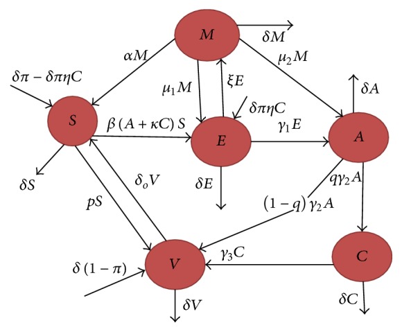
The complete flow diagram of hepatitis B virus transmission model.

3. Equilibria and Basic Reproduction Number

System (3) has the disease-free equilibrium at D _o = (S ^o, 0,0, 0,0); that is, S ^o = (δπ + δ _o)/(δ + δ _o + p). At D ₁ = (S ^∗, E ^∗, A ^∗, C ^∗, M ^∗), the endemic equilibria of system (3) are given by

$$\begin{array}{c}{S}^{\ast }=\frac{\left(\delta +{\gamma }_{\mathrm{1}}+\xi \right)\left(\delta +{\gamma }_{\mathrm{2}}\right)\left(\delta +{\gamma }_{\mathrm{3}}\right)\left(\alpha +\delta +{\mu }_{\mathrm{1}}+{\mu }_{\mathrm{2}}\right)-\left[\delta \pi \eta q{\gamma }_{\mathrm{2}}\left(\xi {\mu }_{\mathrm{2}}+{\gamma }_{\mathrm{1}}\left(\alpha +\delta +{\mu }_{\mathrm{1}}+{\mu }_{\mathrm{2}}\right)\right)+\xi {\mu }_{\mathrm{1}}\left(\delta +{\gamma }_{\mathrm{2}}\right)\left(\delta +{\gamma }_{\mathrm{3}}\right)\right]}{\beta \left(\left(\delta +{\gamma }_{\mathrm{3}}\right)+q\kappa {\gamma }_{\mathrm{2}}\right)\left(\xi {\mu }_{\mathrm{2}}+{\gamma }_{\mathrm{1}}\left(\alpha +\delta +{\mu }_{\mathrm{1}}+{\mu }_{\mathrm{2}}\right)\right)},\\ \\ E^{\ast }=\frac{\left(\delta +{\gamma }_{\mathrm{2}}\right)\left(\alpha +\delta +{\mu }_{\mathrm{1}}+{\mu }_{\mathrm{2}}\right)A^{\ast }}{\left({\gamma }_{\mathrm{1}}\left(\alpha +\delta +{\mu }_{\mathrm{1}}+{\mu }_{\mathrm{2}}\right)+{\mu }_{\mathrm{2}}\xi \right)},\\ \\ C^{\ast }=\frac{q{\gamma }_{\mathrm{2}}{A}^{\ast }}{\left(\delta +{\gamma }_{\mathrm{3}}\right)},\\ \\ M^{\ast }=\frac{\xi \left(\delta +{\gamma }_{\mathrm{2}}\right)A^{\ast }}{\left(\xi {\mu }_{\mathrm{2}}+{\gamma }_{\mathrm{1}}\left(\alpha +\delta +{\mu }_{\mathrm{1}}+{\mu }_{\mathrm{2}}\right)\right)}.\\ \end{array}$$ (5)

The basic reproduction number ℛ ₀ for system (3) can be obtained by using the method in [4]. We obtain the following matrices:

$$\begin{array}{c}F=\left(\begin{array}{cccc}\mathrm{0}& \beta S^o& \beta \kappa S^o& \mathrm{0}\\ \mathrm{0}& \mathrm{0}& \mathrm{0}& \mathrm{0}\\ \mathrm{0}& \mathrm{0}& \mathrm{0}& \mathrm{0}\\ \mathrm{0}& \mathrm{0}& \mathrm{0}& \mathrm{0}\end{array}\right),\\ V\\ =\left(\begin{array}{cccc}\left(\delta +\xi +{\gamma }_{\mathrm{1}}\right)& \mathrm{0}& -\delta \pi \eta & -{\mu }_{\mathrm{1}}\\ -{\gamma }_{\mathrm{1}}& \left(\delta +{\gamma }_{\mathrm{2}}\right)& \mathrm{0}& -{\mu }_{\mathrm{2}}\\ \mathrm{0}& -q{\gamma }_{\mathrm{2}}& \left(\delta +{\gamma }_{\mathrm{3}}\right)& \mathrm{0}\\ -\xi & \mathrm{0}& \mathrm{0}& \left(\alpha +\delta +{\mu }_{\mathrm{1}}+{\mu }_{\mathrm{2}}\right)\end{array}\right).\end{array}$$ (6)

The basic reproduction number ℛ ₀ for (3) is given by

$$\begin{array}{c}{\mathcal{R}}_0=\frac{\left[\beta S^o\left(\delta +{\gamma }_3+\kappa q{\gamma }_2\right)+\delta \pi \eta q{\gamma }_2\right]\left({\mu }_2\xi +{\gamma }_1\left(\alpha +\delta +{\mu }_1+{\mu }_2\right)\right)+{\mu }_1\xi \left(\delta +{\gamma }_2\right)\left(\delta +{\gamma }_3\right)}{\left(\delta +{\gamma }_1+\xi \right)\left(\delta +{\gamma }_2\right)\left(\delta +{\gamma }_3\right)\left(\alpha +\delta +{\mu }_1+{\mu }_2\right)}.\end{array}$$ (7)

Define

$$\begin{array}{c}{\mathcal{R}}_1=\frac{\left[\beta \left(\delta \pi +{\delta }_o\right)\left(\delta +{\gamma }_3+\kappa q{\gamma }_2\right)+\delta \pi \eta q{\gamma }_2\left(\delta +{\delta }_o+p\right)\right]{\gamma }_1}{\left(\delta +{\gamma }_1+\xi \right)\left(\delta +{\gamma }_2\right)\left(\delta +{\gamma }_3\right)\left(\delta +{\delta }_o+p\right)},\\ \\ {\mathcal{R}}_2=\frac{\beta \left(\delta \pi +{\delta }_o\right)\left(\delta +{\gamma }_3+\kappa q{\gamma }_2\right)\xi {\mu }_2+\xi \left(\delta +{\delta }_o+p\right)\left[\delta \pi \eta q{\gamma }_2{\mu }_2+{\mu }_1\left(\delta +{\gamma }_2\right)\left(\delta +{\gamma }_3\right)\right]}{\left(\delta +{\gamma }_1+\xi \right)\left(\delta +{\gamma }_2\right)\left(\delta +{\gamma }_3\right)\left(\delta +{\delta }_o+p\right)\left(\alpha +\delta +{\mu }_1+{\mu }_2\right)},\\ \end{array}$$ (8)

where S ^o = (δπ + δ _o)/(δ + δ _o + p) and ℛ ₀ = ℛ ₁ + ℛ ₂.

4. Stability of Disease-Free Equilibrium (DFE)

In this section, we discuss the local and global stability of system (3) at disease-free equilibrium. We have the following results.

Theorem 1 . —

The disease-free equilibrium D _o of system (3) is locally asymptotically stable if ℛ ₀ < 1 and the conditions (γ ₂ + δ)(γ ₃ + δ) > βS ^o γ ₁ and (γ ₂ + δ) > βS ^o are satisfied; otherwise, they become unstable.

Proof —

At the disease-free equilibrium D _o the corresponding Jacobian matrix J _o(ζ) of system (3) is computed as follows:

(9)

where T ₂ = (δπη + βκS ^o + δ _o). The root −(δ + δ _o + p) of J _o(ζ) is clearly negative; the other roots can be obtained from the following equation:

$$\begin{array}{c}{\lambda }^{\mathrm{4}}+c_{\mathrm{1}}{\lambda }^{\mathrm{3}}+c_{\mathrm{2}}{\lambda }^{\mathrm{2}}+c_{\mathrm{3}}\lambda +c_{\mathrm{4}}=\mathrm{0},\end{array}$$ (10)

where

$$\begin{array}{c}{c}_{\mathrm{1}}=\left({\gamma }_{\mathrm{2}}+\delta \right)+\left({\gamma }_{\mathrm{3}}+\delta \right)+\left(\alpha +\delta +{\mu }_{\mathrm{1}}+{\mu }_{\mathrm{2}}\right)\\ +\left({\gamma }_{\mathrm{1}}+\delta +\xi \right),\\ c_{\mathrm{2}}=\left(\alpha +\delta +{\mu }_{\mathrm{2}}\right)\left({\gamma }_{\mathrm{1}}+\delta +\xi \right)+{\mu }_{\mathrm{1}}\left({\gamma }_{\mathrm{1}}+\delta \right)\\ +\left(\left({\gamma }_{\mathrm{2}}+\delta \right)\left({\gamma }_{\mathrm{3}}+\delta \right)-\beta {\gamma }_{\mathrm{1}}{S}^o\right)\\ +\left(\left({\gamma }_{\mathrm{2}}+\delta \right)+\left({\gamma }_{\mathrm{3}}+\delta \right)\right)\\ ·\left[\left(\alpha +\delta +{\mu }_{\mathrm{1}}+{\mu }_{\mathrm{2}}\right)+\left({\gamma }_{\mathrm{1}}+\delta +\xi \right)\right],\\ c_{\mathrm{3}}=\left[\left({\gamma }_{\mathrm{2}}+\delta \right)+\left({\gamma }_{\mathrm{3}}+\delta \right)\right]{\mu }_{\mathrm{1}}\left({\gamma }_{\mathrm{1}}+\delta \right)\\ +\left(\alpha +\delta +{\mu }_{\mathrm{1}}+{\mu }_{\mathrm{2}}\right)\left(\left({\gamma }_{\mathrm{2}}+\delta \right)\left({\gamma }_{\mathrm{3}}+\delta \right)-\beta {\gamma }_{\mathrm{1}}{S}^o\right)\\ +\left({\gamma }_{\mathrm{2}}+\delta \right)\left(\left(\alpha +\delta \right)\left({\gamma }_{\mathrm{1}}+\delta +\xi \right)+{\mu }_{\mathrm{2}}\left({\gamma }_{\mathrm{1}}+\delta \right)\right)\\ +{\mu }_{\mathrm{2}}\xi \left(\left({\gamma }_{\mathrm{2}}+\delta \right)-\beta S^o\right)+\left({\gamma }_{\mathrm{1}}+\delta +\xi \right)\left({\gamma }_{\mathrm{3}}+\delta \right)\\ ·\left[\left(\alpha +\delta +{\mu }_{\mathrm{2}}\right)+\left({\gamma }_{\mathrm{2}}+\delta \right)\left(\mathrm{1}-{\mathcal{R}}_{\mathrm{1}}\right)\right],\\ c_{\mathrm{4}}=\left({\gamma }_{\mathrm{2}}+\delta \right)\left({\gamma }_{\mathrm{3}}+\delta \right)\left(\alpha +\delta +{\mu }_{\mathrm{1}}+{\mu }_{\mathrm{2}}\right)\left({\gamma }_{\mathrm{1}}+\delta +\xi \right)\\ ·\left(\mathrm{1}-{\mathcal{R}}_{\mathrm{0}}\right).\end{array}$$ (11)

The eigenvalues of the characteristics equation have negative real part if the Routh-Hurwitz condition is satisfied; that is, c _i, i = 1,2, 3,4, with c ₁ c ₂ c ₃ − c ₃ ² − c ₁ ² c ₄ > 0. Therefore, if ℛ ₀ < 1 and (γ ₂ + δ)(γ ₃ + δ) > βS ^o γ ₁ and (γ ₂ + δ) > βS ^o, we get c _i > 0 for i = 1,2, 3,4. Thus, at D _o the disease-free equilibrium of system (3) is locally asymptotically stable if the above conditions are satisfied.

Next, we show the global stability of DFE by using the method in [5].

Theorem 2 . —

The disease-free equilibrium of system (3) is globally asymptotically stable if ℛ ₀ < 1.

Proof —

Consider Y ₁ = S, Y ₂ = (E, A, C, M)^T, and Y = (Y ₁, Y ₂). The invariant domain Γ is clearly a compact positive set. We can present the subsystem Y ₁ = G ₁(Y ₁, 0)(Y ₁ − Y ₁ ^∗) as

$$\begin{array}{c}\dot{S}=-\left(\delta +{\delta }_o+p\right)\left(S-\frac{\delta \pi +{\delta }_o}{\left(\delta +{\delta }_o+p\right)}\right).\end{array}$$ (12)

System (3) represents a linear system which is globally asymptotically stable at Y ₁ ^∗ = (δπ + δ _o)/(δ + δ _o + p). The hypotheses in [5] are satisfied. The matrix G ₂(Y) is given by

$$\begin{array}{c}{G}_{\mathrm{2}}\left(Y\right)=\left(\begin{array}{cccc}-\left(\delta +{\gamma }_{\mathrm{1}}+\xi \right)& \beta S& \beta \kappa S+\delta \pi \eta & {\mu }_{\mathrm{1}}\\ {\gamma }_{\mathrm{1}}& -\left(\delta +{\gamma }_{\mathrm{2}}\right)& \mathrm{0}& {\mu }_{\mathrm{2}}\\ \mathrm{0}& q{\gamma }_{\mathrm{2}}& -\left(\delta +{\gamma }_{\mathrm{3}}\right)& \mathrm{0}\\ \xi & \mathrm{0}& \mathrm{0}& -\left({\mu }_{\mathrm{1}}+{\mu }_{\mathrm{2}}+\delta +\alpha \right)\end{array}\right).\end{array}$$ (13)

Following the hypothesis H ₃ in [5], for any Y ∈ Γ the above matrix G ₂(Y) is Metzler and irreducible. Further, we check the fourth condition H ₄ in [5]. There is a maximum in Γ if S = (δπ + δ _o)/(δ + δ _o + p). This corresponds to disease-free equilibrium and the maximum $G_{\mathrm{2}}(\overline{Y})$ is given by

$$\begin{array}{c}{G}_{\mathrm{2}}\left(\overline{Y}\right)=\left(\begin{array}{cccc}-\left(\delta +{\gamma }_{\mathrm{1}}+\xi \right)& \beta S^o& \beta \kappa S^o+\delta \pi \eta & {\mu }_{\mathrm{1}}\\ {\gamma }_{\mathrm{1}}& -\left(\delta +{\gamma }_{\mathrm{2}}\right)& \mathrm{0}& {\mu }_{\mathrm{2}}\\ \mathrm{0}& q{\gamma }_{\mathrm{2}}& -\left(\delta +{\gamma }_{\mathrm{3}}\right)& \mathrm{0}\\ \xi & \mathrm{0}& \mathrm{0}& -\left({\mu }_{\mathrm{1}}+{\mu }_{\mathrm{2}}+\delta +\alpha \right)\end{array}\right).\end{array}$$ (14)

The last hypothesis H ₅ requires that $\alpha (G_{\mathrm{2}}(\overline{Y}))\le \mathrm{0}.$ We write $G_{\mathrm{2}}(\overline{Y})$ in block form as

$$\begin{array}{c}{G}_{\mathrm{2}}\left(\overline{Y}\right)=\left(\begin{array}{cc}{B}_{\mathrm{1}}& B_{\mathrm{2}}\\ B_{\mathrm{3}}& B_{\mathrm{4}}\end{array}\right),\end{array}$$ (15)

where

$$\begin{array}{c}{B}_{\mathrm{1}}=-\left(\delta +{\gamma }_{\mathrm{1}}+\xi \right),\\ B_{\mathrm{2}}=\left(\beta S^o,\beta \kappa S^o+\delta \pi \eta ,{\mu }_{\mathrm{1}}\right),\\ B_{\mathrm{3}}=\left(\begin{array}{c}{\gamma }_{\mathrm{1}}\\ \mathrm{0}\\ \xi \end{array}\right),\\ B_{\mathrm{4}}\\ =\left(\begin{array}{ccc}-\left(\delta +{\gamma }_{\mathrm{2}}\right)& \mathrm{0}& {\mu }_{\mathrm{2}}\\ q{\gamma }_{\mathrm{2}}& -\left(\delta +{\gamma }_{\mathrm{3}}\right)& \mathrm{0}\\ \mathrm{0}& \mathrm{0}& -\left({\mu }_{\mathrm{1}}+{\mu }_{\mathrm{2}}+\delta +\alpha \right)\end{array}\right).\end{array}$$ (16)

Clearly B ₁ is stable Metzler matrix, so we can write α(B ₄ − B ₃ B ₁ ⁻¹ B ₂) ≤ 0. Let K = B ₄ − B ₃ B ₁ ⁻¹ B ₂.

(17)

The characteristics equation of K are given by

$$\begin{array}{c}{\lambda }^{\mathrm{3}}+l_{\mathrm{1}}{\lambda }^{\mathrm{2}}+l_{\mathrm{2}}\lambda +l_{\mathrm{3}}=\mathrm{0},\end{array}$$ (18)

where

$$\begin{array}{c}{l}_{\mathrm{1}}=\left({\gamma }_{\mathrm{1}}+\delta +\xi \right)\left[\left({\gamma }_{\mathrm{2}}+\delta \right)+\left({\gamma }_{\mathrm{3}}+\delta \right)+\left(\alpha +\delta +{\mu }_{\mathrm{2}}\right)+{\mu }_{\mathrm{1}}\left({\gamma }_{\mathrm{1}}+\delta \right)-\beta {\gamma }_{\mathrm{1}}{S}^o\right],\\ l_{\mathrm{2}}=\left({\gamma }_{\mathrm{2}}+\delta \right)\left({\gamma }_{\mathrm{3}}+\delta \right)\left(\mathrm{1}-{\mathcal{R}}_{\mathrm{1}}\right)+\left(\left({\gamma }_{\mathrm{2}}+\delta \right)+\left({\gamma }_{\mathrm{3}}+\delta \right)\right)\left(\left(\alpha +\delta +{\mu }_{\mathrm{2}}\right)+\frac{{\mu }_{\mathrm{1}}\left({\gamma }_{\mathrm{1}}+\delta \right)}{\left(\gamma +\delta +\xi \right)}\right)\\ +\frac{\beta S^o}{{\left({\gamma }_{\mathrm{1}}+\delta +\xi \right)}^{\mathrm{2}}}\left(\mathrm{2}{\gamma }_{\mathrm{1}}{\mu }_{\mathrm{1}}\xi -\left({\gamma }_{\mathrm{1}}+\delta +\xi \right)·\left(\xi {\mu }_{\mathrm{2}}+{\gamma }_{\mathrm{1}}\left(\alpha +\delta +{\mu }_{\mathrm{1}}+{\mu }_{\mathrm{2}}\right)\left({\gamma }_{\mathrm{1}}+\delta +\xi \right)\right)\right),\\ l_{\mathrm{3}}=\frac{\mathrm{2}{\mu }_{\mathrm{1}}\xi {\gamma }_{\mathrm{1}}}{{\left({\gamma }_{\mathrm{1}}+\delta +\xi \right)}^{\mathrm{2}}}\left[q{\gamma }_{\mathrm{2}}\left(\delta \pi \eta +\beta \kappa S^o\right)+\left({\gamma }_{\mathrm{3}}+\delta \right)\beta S^o\right]\\ +\left({\gamma }_{\mathrm{2}}+\delta \right)\left({\gamma }_{\mathrm{3}}+\delta \right)\times \left(\alpha +\delta +{\mu }_{\mathrm{1}}+{\mu }_{\mathrm{2}}\right)\left(\mathrm{1}-{\mathcal{R}}_{\mathrm{0}}\right).\end{array}$$ (19)

The Routh-Hurwitz criteria ensure that the above characteristics equation has three negative eigenvalues if ℛ ₀ < 1 and the condition l ₁ l ₂ − l ₃ > 0. All the conditions in [5] are satisfied. Thus, we conclude that system (3) at disease-free equilibrium is globally asymptotically stable.

5. Stability EE

In this section, we determine the local and global stability of (3) at endemic equilibrium.

Theorem 3 . —

If ℛ ₀ > 1, then model (3) at endemic equilibrium is locally asymptotically stable.

Proof —

The Jacobian matrix J ^∗ computed at D ₁ is given by

(20)

The characteristics equation at D ₁ is

$$\begin{array}{c}{\lambda }^{\mathrm{5}}+g_{\mathrm{1}}{\lambda }^{\mathrm{4}}+g_{\mathrm{2}}{\lambda }^{\mathrm{3}}+g_{\mathrm{3}}{\lambda }^{\mathrm{2}}+g_{\mathrm{4}}\lambda +g_{\mathrm{5}}=\mathrm{0},\end{array}$$ (21)

where

$$\begin{array}{c}{g}_{\mathrm{1}}=\mathrm{4}\delta +z_{\mathrm{1}}+\alpha +{\gamma }_{\mathrm{1}}+{\gamma }_{\mathrm{2}}+{\gamma }_{\mathrm{3}}+{\mu }_{\mathrm{1}}+{\mu }_{\mathrm{2}}+\xi ,\\ g_{\mathrm{2}}=\left(\alpha +\delta +{\mu }_{\mathrm{1}}+{\mu }_{\mathrm{2}}\right)\left[\left({\gamma }_{\mathrm{1}}+\delta \right)+\left({\gamma }_{\mathrm{2}}+\delta \right)+\left({\gamma }_{\mathrm{3}}+\delta \right)\right]+\xi \left(\alpha +\delta +{\mu }_{\mathrm{2}}\right)+\left[\left(\alpha +\delta +{\mu }_{\mathrm{1}}+{\mu }_{\mathrm{2}}\right)+\left({\gamma }_{\mathrm{1}}+\delta +\xi \right)+\left({\gamma }_{\mathrm{2}}+\delta \right)+\left({\gamma }_{\mathrm{3}}+\delta \right)\right]z_{\mathrm{1}}+\left({\gamma }_{\mathrm{2}}+\delta \right)\\ ·\left[\left({\gamma }_{\mathrm{1}}+\delta +\xi \right)+\left({\gamma }_{\mathrm{3}}+\delta \right)\right]+\left({\gamma }_{\mathrm{3}}+\delta \right)\left({\gamma }_{\mathrm{1}}+\delta +\xi \right)\\ -\left(z_{\mathrm{3}}+{\delta }_o{z}_{\mathrm{2}}\right),\\ g_{\mathrm{3}}=\left(\alpha +\delta +{\mu }_{\mathrm{1}}+{\mu }_{\mathrm{2}}\right)\\ ·\left[\left({\gamma }_{\mathrm{1}}+\delta +\xi \right)\left(\left({\gamma }_{\mathrm{3}}+\delta \right)+\left({\gamma }_{\mathrm{2}}+\delta \right)\right)+\left({\gamma }_{\mathrm{2}}+\delta \right)\left({\gamma }_{\mathrm{3}}+\delta \right)-{\delta }_o{z}_{\mathrm{2}}\right]+z_{\mathrm{2}}\xi \left[\left(\alpha -{\delta }_o\right)-\left({\gamma }_{\mathrm{3}}+\delta \right){\delta }_o-\left({\gamma }_{\mathrm{2}}+\delta \right){\delta }_o\right]+\left({\gamma }_{\mathrm{2}}+\delta \right)\\ ·z_{\mathrm{1}}\left[\left({\gamma }_{\mathrm{1}}+\delta +\xi \right)+\left({\gamma }_{\mathrm{3}}+\delta \right)\right]+\left(\alpha +\delta +{\mu }_{\mathrm{1}}+{\mu }_{\mathrm{2}}\right)\\ ·z_{\mathrm{1}}\left[\left({\gamma }_{\mathrm{1}}+\delta +\xi \right)+\left({\gamma }_{\mathrm{3}}+\delta \right)+\left({\gamma }_{\mathrm{2}}+\delta \right)\right]+\left({\gamma }_{\mathrm{3}}+\delta \right)\\ ·\left({\gamma }_{\mathrm{1}}+\delta +\xi \right)z_{\mathrm{1}}-z_{\mathrm{1}}\left({\mu }_{\mathrm{1}}\xi +z_{\mathrm{3}}\right)-{\gamma }_{\mathrm{1}}{z}_{\mathrm{2}}{z}_{\mathrm{4}}\\ -{\mu }_{\mathrm{1}}\xi \left[\left({\gamma }_{\mathrm{3}}+\delta \right)+\left({\gamma }_{\mathrm{2}}+\delta \right)\right]+\left({\gamma }_{\mathrm{2}}+\delta \right)\left({\gamma }_{\mathrm{3}}+\delta \right)\left({\gamma }_{\mathrm{1}}+\delta +\xi \right)-z_{\mathrm{5}}-z_{\mathrm{3}}\left(\alpha +\delta +{\mu }_{\mathrm{1}}+{\mu }_{\mathrm{2}}\right)-z_{\mathrm{3}}\left({\gamma }_{\mathrm{3}}+\delta \right)\\ -z_{\mathrm{6}},\\ g_{\mathrm{4}}=\left({\gamma }_{\mathrm{2}}+\delta \right)\left({\gamma }_{\mathrm{3}}+\delta \right)\left(\alpha +\delta +{\mu }_{\mathrm{1}}+{\mu }_{\mathrm{2}}\right)\left({\gamma }_{\mathrm{1}}+\delta +\xi \right)\\ -\left({\gamma }_{\mathrm{2}}+\delta \right){\delta }_o\left(\alpha +\delta +{\mu }_{\mathrm{1}}+{\mu }_{\mathrm{2}}\right)z_{\mathrm{2}}-\left({\gamma }_{\mathrm{3}}+\delta \right){\delta }_o\left(\alpha +\delta +{\mu }_{\mathrm{1}}+{\mu }_{\mathrm{2}}\right)z_{\mathrm{2}}+\xi \left({\gamma }_{\mathrm{2}}+\delta \right)z_{\mathrm{2}}\left(\alpha -{\delta }_o\right)+z_{\mathrm{2}}\xi \left({\gamma }_{\mathrm{3}}+\delta \right)\left(\alpha -{\delta }_o\right)-{\mu }_{\mathrm{1}}\xi \left({\gamma }_{\mathrm{2}}+\delta \right)z_{\mathrm{1}}-{\mu }_{\mathrm{1}}\xi \left({\gamma }_{\mathrm{3}}+\delta \right)z_{\mathrm{1}}\\ -\left({\gamma }_{\mathrm{2}}+\delta \right)\left({\gamma }_{\mathrm{3}}+\delta \right){\delta }_o{z}_{\mathrm{2}}-z_{\mathrm{3}}\left(\alpha +\delta +{\mu }_{\mathrm{1}}+{\mu }_{\mathrm{2}}\right)z_{\mathrm{1}}\\ +\left[\left({\gamma }_{\mathrm{2}}+\delta \right)+\left({\gamma }_{\mathrm{3}}+\delta \right)\right]\left(\alpha +\delta +{\mu }_{\mathrm{1}}+{\mu }_{\mathrm{2}}\right)\left({\gamma }_{\mathrm{1}}+\delta +\xi \right)z_{\mathrm{1}}-{\gamma }_{\mathrm{1}}\left({\gamma }_{\mathrm{3}}+\delta \right)z_{\mathrm{2}}{z}_{\mathrm{4}}-z_{\mathrm{1}}{z}_{\mathrm{5}}+\left({\gamma }_{\mathrm{2}}+\delta \right)\left({\gamma }_{\mathrm{3}}+\delta \right)\\ ·\left(\alpha +\delta +{\mu }_{\mathrm{1}}+{\mu }_{\mathrm{2}}\right)z_{\mathrm{1}}+\left({\gamma }_{\mathrm{2}}+\delta \right)\left({\gamma }_{\mathrm{3}}+\delta \right)\left({\gamma }_{\mathrm{1}}+\delta +\xi \right)z_{\mathrm{1}}-{\mu }_{\mathrm{2}}\xi z_{\mathrm{2}}{z}_{\mathrm{4}}-z_{\mathrm{3}}\left({\gamma }_{\mathrm{3}}+\delta \right)z_{\mathrm{1}}-z_{\mathrm{1}}{z}_{\mathrm{6}}-z_{\mathrm{1}}{z}_{\mathrm{5}}\\ -{\gamma }_{\mathrm{1}}\left(\alpha +\delta +{\mu }_{\mathrm{1}}+{\mu }_{\mathrm{2}}\right)z_{\mathrm{2}}{z}_{\mathrm{4}}+{\mu }_{\mathrm{1}}\xi \left({\gamma }_{\mathrm{2}}+\delta \right)\left({\gamma }_{\mathrm{3}}+\delta \right)\\ -\left(\alpha +\delta +{\mu }_{\mathrm{1}}+{\mu }_{\mathrm{2}}\right)z_{\mathrm{5}}-z_{\mathrm{7}}-z_{\mathrm{3}}\left({\gamma }_{\mathrm{3}}+\delta \right)\left(\alpha +\delta +{\mu }_{\mathrm{1}}+{\mu }_{\mathrm{2}}\right)-z_{\mathrm{6}}\left({\gamma }_{\mathrm{3}}+\delta \right),\\ g_{\mathrm{5}}=-\left({\gamma }_{\mathrm{2}}+\delta \right)\left({\gamma }_{\mathrm{3}}+\delta \right){\delta }_o\left(\alpha +\delta +{\mu }_{\mathrm{1}}+{\mu }_{\mathrm{2}}\right)z_{\mathrm{2}}\\ +\xi \left({\gamma }_{\mathrm{2}}+\delta \right)\left({\gamma }_{\mathrm{3}}+\delta \right)z_{\mathrm{2}}\left(\alpha -{\delta }_o\right)+\left({\gamma }_{\mathrm{2}}+\delta \right)\left({\gamma }_{\mathrm{3}}+\delta \right)\\ ·\left(\alpha +\delta +{\mu }_{\mathrm{1}}+{\mu }_{\mathrm{2}}\right)\left({\gamma }_{\mathrm{1}}+\delta +\xi \right)z_{\mathrm{1}}-{\mu }_{\mathrm{1}}\xi \left({\gamma }_{\mathrm{2}}+\delta \right)\\ ·\left({\gamma }_{\mathrm{3}}+\delta \right)z_{\mathrm{1}}-\left(\alpha +\delta +{\mu }_{\mathrm{1}}+{\mu }_{\mathrm{2}}\right)z_{\mathrm{5}}{z}_{\mathrm{1}}-z_{\mathrm{1}}{z}_{\mathrm{7}}\\ -z_{\mathrm{3}}\left({\gamma }_{\mathrm{3}}+\delta \right)\left(\alpha +\delta +{\mu }_{\mathrm{1}}+{\mu }_{\mathrm{2}}\right)z_{\mathrm{1}}-z_{\mathrm{6}}{z}_{\mathrm{1}}\\ -{\gamma }_{\mathrm{1}}{z}_{\mathrm{2}}q{\gamma }_{\mathrm{2}}\left(\alpha +\delta +{\mu }_{\mathrm{1}}+{\mu }_{\mathrm{2}}\right)z_{\mathrm{8}}-{\mu }_{\mathrm{2}}\xi q{\gamma }_{\mathrm{2}}{z}_{\mathrm{2}}{z}_{\mathrm{8}}\\ -{\gamma }_{\mathrm{1}}\left({\gamma }_{\mathrm{3}}+\delta \right)\left(\alpha +\delta +{\mu }_{\mathrm{1}}+{\mu }_{\mathrm{2}}\right)z_{\mathrm{2}}{z}_{\mathrm{4}}-{\mu }_{\mathrm{2}}\xi \left({\gamma }_{\mathrm{3}}+\delta \right)\\ ·z_{\mathrm{2}}{z}_{\mathrm{4}},\end{array}$$ (22)

where z ₁ = (δ + δ _o + p) + β(A ^∗ + κC ^∗), z ₂ = β(A ^∗ + κC ^∗), z ₃ = βγ ₁ S ^∗, z ₄ = (δ _o + βS ^∗), z ₅ = γ ₁ qγ ₂(πδη + βκS ^∗), z ₆ = βμ ₂ ξS ^∗, z ₇ = μ ₂ ξqγ ₂(πδη + βκS ^∗), and z ₈ = (πδη + δ _o + βκS ^∗). The characteristics equation will give negative roots if the following conditions are satisfied:

• (i) g ₁, g ₂, g ₃, g ₄, g ₅ > 0,
• (ii) g ₁ g ₂ − g ₃ > 0,
• (iii) g ₄ g ₅(g ₃(g ₁ g ₂ − g ₃) − g ₁ ² g ₄) > 0,
• (iv) g ₅ ²(2g ₁ g ₄ − g ₂(g ₁ g ₂ − g ₃) − g ₅) > 0.

Conditions (i) and (ii) are easy to satisfy. If conditions (iii) and (iv) are satisfied; then the characteristics equation given above will give negative eigenvalues. Thus, it follows from Routh-Hurwitz criteria that system (3) is locally asymptotically stable at D ₁.

Next result shows the global stability of the endemic equilibrium D ₁ of system (3) for special case when μ ₁ = 0 and α = 0. We have the following result.

Theorem 4 . —

The endemic equilibrium D ₁ of system (3) is globally asymptotically stable if condition (30) holds.

Proof —

We define the Lyapunov function in the following form:

$$\begin{array}{c}\mathcal{V}=w_{\mathrm{1}}\left(S-S^{\ast }-S^{\ast }\log \frac{S^{\ast }}{S}\right)\\ +w_{\mathrm{2}}\left(E-E^{\ast }-E^{\ast }\log \frac{E^{\ast }}{E}\right)+w_{\mathrm{3}}A+w_{\mathrm{4}}C+w_{\mathrm{5}}M.\end{array}$$ (23)

The time durative of 𝒱 is

$$\begin{array}{c}{\mathcal{V}}^{\prime }=w_{\mathrm{1}}\left(\mathrm{1}-\frac{S^{\ast }}{S}\right)S^{\prime }+w_{\mathrm{2}}\left(\mathrm{1}-\frac{E^{\ast }}{E}\right)E^{\prime }+w_{\mathrm{3}}{A}^{\prime }\\ +w_{\mathrm{4}}{C}^{\prime }+w_{\mathrm{5}}{M}^{\prime }.\end{array}$$ (24)

The coefficients w ₁,…, w ₅ are positive and will be determined later. At endemic steady state the first equation of (3) is given by

$$\begin{array}{c}\delta \pi +{\delta }_o=\delta \pi \eta C^{\ast }+\left(\delta +p\right)S^{\ast }+\beta \left(A^{\ast }+\kappa C^{\ast }\right)S^{\ast }\\ +{\delta }_o{X}^{\ast }.\end{array}$$ (25)

Using (25) and the S equation (3) we obtain

$$\begin{array}{c}{w}_{\mathrm{1}}\left(\mathrm{1}-\frac{S^{\ast }}{S}\right)S^{\prime }=w_{\mathrm{1}}\left(\mathrm{1}-\frac{S^{\ast }}{S}\right)\left[\delta \pi \eta C^{\ast }+\left(\delta +p\right)S^{\ast }+\beta \left(A^{\ast }+\kappa C^{\ast }\right)S^{\ast }+{\delta }_o{X}^{\ast }\right]-w_{\mathrm{1}}\left[\delta \pi \eta C+\left(\delta +p\right)S+\beta \left(A+\kappa C\right)S+{\delta }_{o}X\right]+w_{\mathrm{1}}\\ ·\frac{S^{\ast }}{S}\left[\delta \pi \eta C\left(t\right)+\left(\delta +p\right)S\left(t\right)+\beta \left(A\left(t\right)+\kappa C\left(t\right)\right)S\left(t\right)+{\delta }_{o}X\right].\end{array}$$ (26)

Similarly,

$$\begin{array}{c}{w}_{\mathrm{2}}\left(\mathrm{1}-\frac{E^{\ast }}{E}\right)E^{\prime }=w_{\mathrm{2}}\left[\beta \left(A\left(t\right)+\kappa C\left(t\right)\right)S\left(t\right)-\left(\delta +{\gamma }_{\mathrm{1}}+\xi \right)E\left(t\right)+\delta \pi \eta C\left(t\right)\right]-w_{\mathrm{2}}\frac{E^{\ast }}{E}\beta \left(A\left(t\right)+\kappa C\left(t\right)\right)S\left(t\right)+w_{\mathrm{2}}\beta \left(A^{\ast }+\kappa C^{\ast }\right)S^{\ast }+w_{\mathrm{2}}\delta \pi \eta C^{\ast }\\ +\delta \pi \eta C\left(t\right)\frac{E^{\ast }}{E}.\end{array}$$ (27)

Using the values of (26) and (27) and the last three equations of system (3) and substituting in (24) we obtain

$$\begin{array}{c}{\mathcal{V}}^{\prime }=w_{\mathrm{1}}\left(\mathrm{1}-\frac{S^{\ast }}{S}\right)\left[\delta \pi \eta C^{\ast }+\left(\delta +p\right)S^{\ast }+\beta \left(A^{\ast }+\kappa C^{\ast }\right)S^{\ast }+{\delta }_o{X}^{\ast }\right]-w_{\mathrm{1}}\delta \pi \eta C-w_{\mathrm{1}}\left(\delta +p\right)S-w_{\mathrm{1}}\beta \left(A+\kappa C\right)S-w_{\mathrm{1}}{\delta }_{o}X+w_{\mathrm{1}}\frac{S^{\ast }}{S}\\ ·\delta \pi \eta C\left(t\right)+w_{\mathrm{1}}\left(\delta +p\right)S+w_{\mathrm{1}}\beta \left(A+\kappa C\right)S\\ +w_{\mathrm{1}}{\delta }_{o}X+w_{\mathrm{2}}\left[\beta \left(A+\kappa C\right)S-\left(\delta +{\gamma }_{\mathrm{1}}+\xi \right)E+\delta \pi \eta C\right]-w_{\mathrm{2}}\frac{E^{\ast }}{E}\beta \left(A+\kappa C\right)S+w_{\mathrm{2}}\beta \left(A^{\ast }+\kappa C^{\ast }\right)\\ ·S^{\ast }+w_{\mathrm{2}}\delta \pi \eta C^{\ast }+w_{\mathrm{2}}\delta \pi \eta C\frac{E^{\ast }}{E}.\end{array}$$ (28)

After implication we obtain

$$\begin{array}{c}{\mathcal{V}}^{\prime }=-\frac{q{\gamma }_{\mathrm{2}}\left({\mu }_{\mathrm{2}}\xi +{\gamma }_{\mathrm{1}}\left({\mu }_{\mathrm{1}}+{\mu }_{\mathrm{2}}+\delta +\alpha \right)\right)}{\left({\mu }_{\mathrm{1}}+{\mu }_{\mathrm{2}}+\delta +\alpha \right)\left(\delta +{\gamma }_{\mathrm{1}}+\xi \right)}\left(\delta +p\right)\\ ·\frac{{\left(S-S^{\ast }\right)}^{\mathrm{2}}}{S}-\frac{q{\gamma }_{\mathrm{2}}\left({\mu }_{\mathrm{2}}\xi +{\gamma }_{\mathrm{1}}\left({\mu }_{\mathrm{1}}+{\mu }_{\mathrm{2}}+\delta +\alpha \right)\right)}{\left({\mu }_{\mathrm{1}}+{\mu }_{\mathrm{2}}+\delta +\alpha \right)\left(\delta +{\gamma }_{\mathrm{1}}+\xi \right)}\\ ·\beta S^{\ast }{A}^{\ast }\times \left(-\mathrm{2}+\frac{S^{\ast }}{S}+\frac{AS{E}^{\ast }}{A^{\ast }{S}^{\ast }E}\right)\\ -\frac{q{\gamma }_{\mathrm{2}}\left({\mu }_{\mathrm{2}}\xi +{\gamma }_{\mathrm{1}}\left({\mu }_{\mathrm{1}}+{\mu }_{\mathrm{2}}+\delta +\alpha \right)\right)}{\left({\mu }_{\mathrm{1}}+{\mu }_{\mathrm{2}}+\delta +\alpha \right)\left(\delta +{\gamma }_{\mathrm{1}}+\xi \right)}\beta S^{\ast }\kappa C^{\ast }\left(-\mathrm{2}+\frac{S^{\ast }}{S}+\frac{CS{E}^{\ast }}{C^{\ast }{S}^{\ast }E}\right)\\ -\frac{q{\gamma }_{\mathrm{2}}\left({\mu }_{\mathrm{2}}\xi +{\gamma }_{\mathrm{1}}\left({\mu }_{\mathrm{1}}+{\mu }_{\mathrm{2}}+\delta +\alpha \right)\right)}{\left({\mu }_{\mathrm{1}}+{\mu }_{\mathrm{2}}+\delta +\alpha \right)\left(\delta +{\gamma }_{\mathrm{1}}+\xi \right)}\left(-\mathrm{2}+\frac{S^{\ast }}{S}+\frac{C}{C^{\ast }}\frac{E^{\ast }}{E}-\frac{C}{C^{\ast }}\frac{S^{\ast }}{S}\right)\delta \pi \eta C^{\ast }-\left(\delta +{\gamma }_{\mathrm{2}}\right)\left(\delta +{\gamma }_{\mathrm{3}}\right)C\\ -\frac{q{\gamma }_{\mathrm{2}}\left({\mu }_{\mathrm{2}}\xi +{\gamma }_{\mathrm{1}}\left({\mu }_{\mathrm{1}}+{\mu }_{\mathrm{2}}+\delta +\alpha \right)\right)}{\left({\mu }_{\mathrm{1}}+{\mu }_{\mathrm{2}}+\delta +\alpha \right)\left(\delta +{\gamma }_{\mathrm{1}}+\xi \right)}{\delta }_o{X}^{\ast }\left(-\mathrm{1}+\frac{S^{\ast }}{S}+\frac{X}{X^{\ast }}-\frac{X}{X^{\ast }}\frac{S^{\ast }}{S}\right),\end{array}$$ (29)

where the constants w ₁,…, w ₅ are chosen as w ₄ = (δ + γ ₂), w ₃ = qγ ₂, w ₅ = qγ ₂ μ ₂/(μ ₁ + μ ₂ + δ + α), w ₂ = w ₁ = qγ ₂(μ ₂ ξ + γ ₁(μ ₁ + μ ₂ + δ + α))/(μ ₁ + μ ₂ + δ + α)(δ + γ ₁ + ξ), and X = S + E + A + C + M, X ^∗ = S ^∗ + E ^∗ + A ^∗ + C ^∗ + M ^∗.

Equation (29) 𝒱′ ≤ 0 if the following inequalities are satisfied:

$$\begin{array}{c}\left(-\mathrm{2}+\frac{S^{\ast }}{S}+\frac{C}{C^{\ast }}\frac{E^{\ast }}{E}-\frac{C}{C^{\ast }}\frac{S^{\ast }}{S}\right)\ge \mathrm{0},\\ \\ \left(-\mathrm{2}+\frac{S^{\ast }}{S}+\frac{CS{E}^{\ast }}{C^{\ast }{S}^{\ast }E}\right)\ge \mathrm{0},\\ \\ \left(-\mathrm{2}+\frac{S^{\ast }}{S}+\frac{C}{C^{\ast }}\frac{E^{\ast }}{E}-\frac{C}{C^{\ast }}\frac{S^{\ast }}{S}\right)\ge \mathrm{0},\\ \\ \left(-\mathrm{1}+\frac{S^{\ast }}{S}+\frac{X}{X^{\ast }}-\frac{X}{X^{\ast }}\frac{S^{\ast }}{S}\right)\ge \mathrm{0}.\\ \end{array}$$ (30)

The endemic equilibrium D ₁ of system (3) is said to be globally asymptotically stable if condition (30) holds.

6. Numerical Simulation

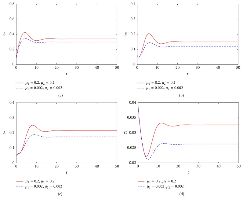
This section deals with the numerical solution of model (3). The numerical results for model (3) are presented in Figures 2 –8. In this paper, the value for α and ξ is taken between 0 and 1. The rest of the parameters values are taken from [1], except those mentioned in the figures. Figure 1 shows the population behavior of incidentals when μ ₁ = 0.1 and μ ₂ = 0.1. Figure 3 represents the population of incisiveness when μ ₁ = 0.2 and μ ₂ = 0.2. In Figures 2 and 3, the individuals of carriers decrease sharply. For μ ₁ = 0.001 and μ ₂ = 0.02, we present Figure 4. Figure 5 is population behavior of individuals when μ ₁ = 0.1 and μ ₂ = 0.2. Figures 6 and 7, respectively, represent the population of carriers individuals for different values of parameters. The population behavior of susceptible, exposed, acute, and carriers individuals for different parameters is presented in Figure 8. The numerical results from Figures 2 to 8 show when there is a decrease in the value of suggested parameters, and the population of individuals in the host decreases sharply.

Figure 2.

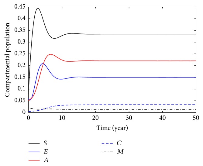
Population behavior of individuals when μ ₁ = 0.1, μ ₂ = 0.1.

Figure 3.

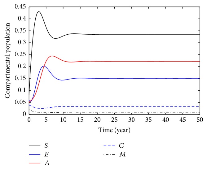
Population behavior of individuals when μ ₁ = 0.2, μ ₂ = 0.2.

Figure 4.

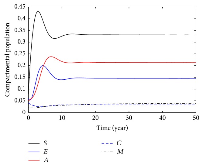
Population behavior of individuals when μ ₁ = 0.01,  μ ₂ = 0.02.

Figure 5.

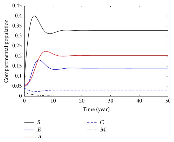
Population behavior of individuals when μ ₁ = 0.1, μ ₂ = 0.2.

Figure 6.

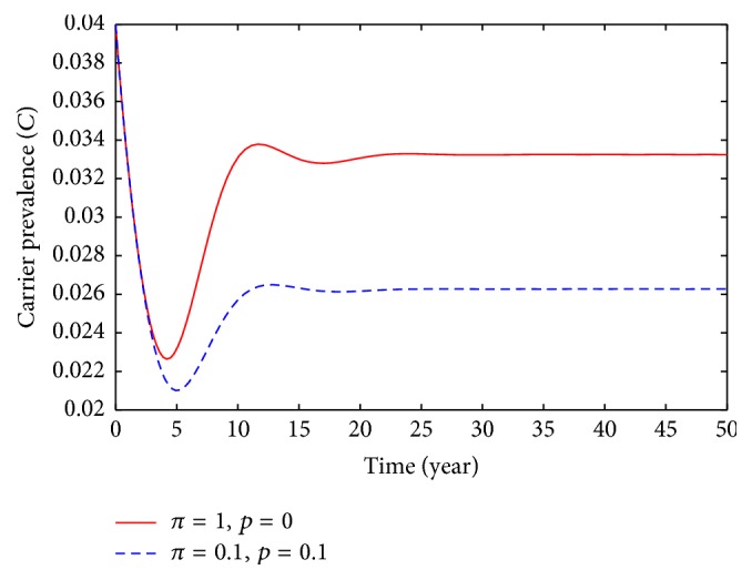
Population behavior of carriers individuals: solid line, π = 1, p = 0; dashed π = 0.1, p = 0.1.

Figure 7.

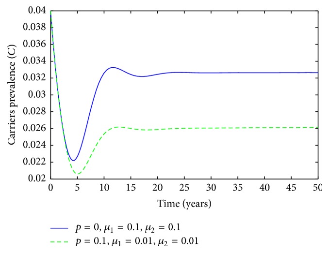
Population behavior of carriers individuals: solid line p = 0, μ ₁ = 0.1, and μ ₂ = 0.1; dashed p = 0.1, μ ₁ = 0.01, and μ ₂ = 0.01.

Figure 8.

Population behavior of susceptible, exposed, acute, and carriers individuals: solid line μ ₁ = 0.2, μ ₂ = 0.2; dashed μ ₁ = 0.002, μ ₂ = 0.002.

7. Conclusion

In this corrigendum, we make all the necessary changes to the published paper [1], which are highlighted in the comment papers [2, 3]. We added the parameter α, a rate from migrated class to susceptible, and ξ is the rate of flow from exposed to migrated classes. Further, the basic reproduction number has been investigated. The mathematical results for the revised model are presented successfully.

References

- 1.Khan M. A., Islam S., Arif M., Ul Haq Z. Transmission model of hepatitis b virus with the migration effect. BioMed Research International. 2013;2013:10. doi: 10.1155/2013/150681.150681 [DOI] [PMC free article] [PubMed] [Google Scholar]
- 2.Zeb A., Zaman G. Comment on ‘transmission model of hepatitis B virus with migration effect’. BioMed Research International. 2015;2015:4. doi: 10.1155/2015/492513.492513 [DOI] [PMC free article] [PubMed] [Google Scholar]
- 3.Lashari A. A. Comment on ‘transmission model of Hepatitis B virus with the migration effect’. BioMed Research International. 2015;2015:2. doi: 10.1155/2015/469240.469240 [DOI] [PMC free article] [PubMed] [Google Scholar]
- 4.van den Driessche P., Watmough J. Reproduction numbers and sub-threshold endemic equilibria for compartmental models of disease transmission. Mathematical Biosciences. 2002;180:29–48. doi: 10.1016/S0025-5564(02)00108-6. [DOI] [PubMed] [Google Scholar]
- 5.Kamgang J. C., Sallet G. Computation of threshold conditions for epidemiological models and global stability of the disease-free equilibrium (DFE) Mathematical Biosciences. 2008;213(1):1–12. doi: 10.1016/j.mbs.2008.02.005. [DOI] [PubMed] [Google Scholar]