Finding Significant Stress Episodes in a Discontinuous Time Series of Rapidly Varying Mobile Sensor Data

Abstract

Management of daily stress can be greatly improved by delivering sensor-triggered just-in-time interventions (JITIs) on mobile devices. The success of such JITIs critically depends on being able to mine the time series of noisy sensor data to find the most opportune moments. In this paper, we propose a time series pattern mining method to detect significant stress episodes in a time series of discontinuous and rapidly varying stress data. We apply our model to 4 weeks of physiological, GPS, and activity data collected from 38 users in their natural environment to discover patterns of stress in real-life. We find that the duration of a prior stress episode predicts the duration of the next stress episode and stress in mornings and evenings is lower than during the day. We then analyze the relationship between stress and objectively rated disorder in the surrounding neighborhood and develop a model to predict stressful episodes.

INTRODUCTION

Recent advances in wearable sensors and computational modeling have made it feasible to obtain continuous assessment of stress in the natural environment [32, 34, 52]. They have inspired research on visualization of dense time series of stress measurements together with associated contexts (e.g., location, activity, driving, etc.) that may inform the content and timing of just-in-time stress interventions [59].

Given the widespread adverse health consequences of stress (both in the short term and in the long term) [12,42,45,48,57], these advances hold tremendous promise to improve public health and wellbeing. But delivering a sensor-triggered stress intervention (e.g., breathing or relaxation exercises) is feasible only if there exists a method to detect clinically significant stress episodes in real time that can be used to trigger the intervention at most opportune moments.

To trigger a reactive stress intervention, we need to locate major stress episodes in the sensor data stream. This introduces several challenges. First, stress measurements obtained from sensors usually have to be inferred from physiological data, which by their very nature is rapidly varying, similar to real-time tracking of stock prices. Second, unlike stock-price data, the time series of stress is discontinuous due to factors such as sensor detachment and wireless losses [51, 55]. Third, sensor measurements are frequently confounded by physical activity (23% of the time [55]), that need to be filtered out for an accurate assessment of stress.

Another set of challenges concerns the triggering of the intervention. First, the decision to trigger must be made quickly so the intervention can be effective. Hence, simple methods that can be efficiently implemented on mobile devices are needed. Second, too-frequent prompts of an intervention can lead to alarm fatigue [38] and render the system useless. Ideally, the intervention policy should be personalized to the tolerance level of the individual and the frequency of intervention (e.g., once per day) desired by the user.

In this paper, we take first steps towards the development of such JITI and develop time-series-pattern mining methods to detect significant stress episodes in discontinuous ambulatory data. The goal of this work is to establish the foundation on which a just-in-time stress intervention can be developed.

For model development and application, we use data collected in a 4-week field study in 38 opioid-dependent poly-drug users receiving opioid agonist maintenance treatment, all of whom were in a larger trial investigating individual and environmental influences on drug use. Each participant wore wireless physiological sensors for 10+ hours per day, from which we obtained a continuous measure of stress [34].

In brief, we first developed methods to deal with physical activity and discontinuities in the time-series data. We then applied the cStress model [34], imputed the missing data, and validated the output of cStress (together with its imputation) against self-reported stress. Next, we trained a stock prediction method called Moving Average Convergence Divergence (MACD) [3] to locate the time of an increase in stress in rapidly varying continuous time-series data. We estimated the probability distribution of the likelihood of stress assessments and the probability distribution of stress durations (in the smoothed time series) to personalize the algorithm for each individual. The threshold on stress likelihood can correspond to tolerance level, and the duration can be selected to meet the expected intervention frequency preference.

We assessed relationships between stress and the neighborhood environment with independently obtained data from the Neighborhood Inventory for Environmental Typology (NIfETy) [25]. Finally, as a next step toward developing a just-in-time proactive stress intervention, we investigated the feasibility of predicting whether a rapid rise in stress would lead to a significant stress episode from spatio-temporal context and the users’ prior history. The development and deployment of a JITI represents a future research opportunity.

RELATED WORKS

The first category of related works are the ones on stress monitoring. Assessment of stress and physiology can be obtained episodically when a user interacts with a device or continuously via sensors on the body or in the user’s environment. Examples of the former include capturing ECG from a smartphone camera (during gaming [26]) or from electrodes embedded on smartphone jackets (e.g., Alivecore), hand arm dynamics from the computer mouse [61], and pressure from pressure sensitive keyboard and mouse [28]. Physiology can be obtained continuously from wearable physiological sensors [19]. Stress detection can be done from a variety of physiological parameters including ECG and respiration [34, 52], electrodermal response [43], photoplethysmography from fingertip [40], or near-infrared spectroscopy from forehead [29]. Our method can be applied to stress measurements obtained from any of the above methods.

The second category of works are those that assess interruptibility, workload, or availability to decide when to deliver a prompt for intervention, self-report, or phone call [22, 35, 36, 62]. A recent work [58] proposed a model that uses stress, time, location, and the current context to determine the availability or interruptibility of users, in their natural environment, to respond to randomly triggered self-report prompts. It found that users are least available at work and during driving, and most available when walking outside. These works are complementary to ours. Once a trigger for intervention has been generated by our model, it should be delivered to the user only when they are determined as being physically, cognitively, and socially available.

The third category includes works on stress interventions. An example is a reflective intervention called AffectAura [44] that logs physiological state using audio, visual, sensors, and user activities and aims to support reflection via visualization. Visualization is replaced by a wearable butterfly in [41] that helps users reflect on their stress level and regulate it. Textiles have been designed that can actuate in response to stress [14]. These complementary works indicate interesting intervention possibilities, if appropriate methods such as ours can reliably detect stress episodes in real-life.

The fourth category of related works are sensor-triggered JITIs that have emerged in other contexts. For example, [9] presented a JITI to prevent emotional food intake. Another example is [53] that proposed a system where earpieces (to monitor chewing and swallowing), augmented-reality glasses (for capturing food consumed) and a physiological sensor (for heart rate) are connected to a mobile-phone application that processes the data and gives feedback to the user. Sensor-triggered JITIs have also been proposed for preventive maintenance of a plant (see a review in [11]) and for GPS-based vehicle navigation [2, 4]. But, none of these methods can be used directly to mine the time series of stress to find significant stress episodes.

The closest related works are those that aim to discover or predict stress episodes from time series of physiological data. MoodLight [43] finds episodes of arousal from electrodermal activity (EDA) in the lab environment and regulates the color of a desk lamp to reflect the user’s stress level. When users reduce their stress level, the light color changes to blue. In [37], the authors present a method to predict the time series of heart-rate variability (HRV) using a first-order Hidden Markov Model. The algorithm was tested in a simulated patient environment using a beta distribution (α = 0.1 and β = 1). In contrast to these works, our model addresses real-life challenges of discontinuity and rapid variability.

DATA DESCRIPTION

We used data collected as part of a larger outpatient study of relationships among stress, addictive behaviors, and daily activities. The parent study, and this substudy, were approved by the Institutional Review Board (IRB), and all participants provided written informed consent. The participant demographics, study setup, and the data we collected appear below.

Devices and Sensor Measurements

Sensor Suite

During the study, participants wore a wireless suite of physiological sensors under their clothes. The sensor suite consisted of an unobtrusive, flexible band worn around the chest. It provided respiration data by measuring the expansion and contraction of the chest via inductive plethysmography (RIP) and included a two-lead electrocardiograph (ECG), and a 3-axis accelerometer. The measurements were transmitted wirelessly using ANT radio [1] to an Android smartphone. The sampling rates for the sensors were 128 Hz for ECG, 64 Hz for respiration, 32 Hz for each accelerometer axis. They were downsampled at the sensor before wireless transmission at the rate of 28 packets/second, where each packet has 5 samples.

Mobile Phone

Each participant also carried a smartphone. It received and stored data from the sensors; it also sampled and stored data from its own sensors (e.g., accelerometers).

Field Study Procedure

Participants were trained in the proper use of the devices. They were shown how to remove the sensors before going to bed and how to put them back on correctly the next morning. They were also asked to take them off during showers and any contact sport. Participants received an overview of the smartphone software’s user interface. Once the study coordinator felt that participants understood the technology, they left the research clinic and went about their normal lives. Participants were asked to wear the sensors during their waking hours, complete self-reported questionnaires when prompted, and record instances of drug use and craving on the phone.

Participants were asked to return to the research clinic daily. The study coordinator uploaded the data collected the previous day and reviewed the physiological measurements to ensure that sensors were working and were being worn properly. On the final day, participants returned study equipment and completed an Equipment and Experience Questionnaire. Finally, participants were debriefed on their experiences and comfort with the study.

We recruited 38 polydrug users (age 41 ± 10 years, 11 female, 6 dropped out) who agreed to wear the sensor suite. Because drug use does not occur every day in all these users, we conducted the study for four weeks to maximize the likelihood of capturing real-life drug use events.

Compensation

Participants received $10/day for wearing the sensors (and $5 bonus for 14+ hours of wearing), carrying the smartphone, and completing device-prompted questionnaires consisting of 32 items. In total, participants were paid up to $380 plus bonus (if any) for four weeks of participation.

Self-report

The smartphone initiated Ecological Momentary Assessment (EMA) questionnaires at random times. The 32-item EMA asked participants to rate their subjective assessment of affect on a 6-point scale. In addition, participants were asked about the presence of drug and smoking cues.

Data Collected

Participants wore the physiological sensors and carried the smartphone for 12.52 hours each day in their daily, free-living condition. Due to sensor detachment, displacement, loosening, and wireless loss between phone and the sensor, some of the ECG data were not of acceptable quality. We computed the amount of unacceptable ECG data using a method proposed in [55] and discarded them. Acceptable ECG data were obtained 10.54 hours per day on average (around 10,447 hours of data in total); these were the data we used for stress inference. We observed that most of the participants wore the sensor and contributed data between 6:00 AM to 8:00 PM of a day. A total of 5,755 EMA responses were collected (5.8/day), with a compliance rate of 88.0%.

STRESS INFERENCE FROM PHYSIOLOGICAL DATA

In this section, we describe the procedure we used to infer physiological stress from wearable sensors. We adapt a recent model called cStress proposed in [34].

cStress Model for Stress Assessment

The cStress model uses electrocardiogram (ECG) and respiration data to infer stress. This model is applied to a set of features collected from a minute’s worth of sensor measurements, whereby consecutive minutes are non-overlapping, and it determines whether that minute’s sensor readings correspond to a physiological response to stressors. The model includes 80^th percentile of R-R intervals and Heart-Rate Variability (HRV) from the ECG data, and the mean IE ratio and the median of Stretch from the respiration data [34]. This model was shown to classify stress and non-stress minutes with 95% accuracy on independent subject validation (different from training set) in lab stress testing. It also showed that using HRV measure alone from ECG, as has been the case in several prior works [46, 47], leads to a significantly lower F1 score (from 0.78 to 0.56). Finally, the model was evaluated against self-report from independent subjects in the field and was found to have a F1 score of 0.71 [34]. We modified the model to generate stress measurements every five seconds from overlapping windows to get a smoother time series.

Inferred Measures of Stress

The cStress model provides a continuous measure of stress, scaled to be between 0 and 1, for every 5 seconds of overlapping one-minute sensor data. This time-series of 5-second probability-like measures of stress, for a particular participant, is referred to hereafter as “stress likelihood.”

To assess stress within intervals longer than a minute, we use a different measure, called “stress density,” which accounts for likely variation in contexts and activities (e.g. morning vs. afternoon, driving vs. home). We define stress density as the area under the stress-likelihood time-series divided by the length of the interval.

REDUCING THE IMPACT OF CONFOUNDING FACTORS

Although physiology is affected by several kinds of events in daily life, the main confounder for stress assessment is physical activity. To isolate data affected by activity, we first detect physical activity from chest-worn 3-axis accelerometer data, using an existing model [55]. Second, we estimate the time it takes for physiology to recover from the effect of a just concluded activity episode. Both data are then excluded.

Physiological readings generally return to baseline within 2 minutes after physical activity (unless the activity is especially intense) [20]. However, the majority of activity episodes in our daily life are of short durations. Although our participants were physically active 22.7% of their sensor-wearing time, 95% of their activities lasted less than 2.1 minutes. Discarding 2 minutes of data after each activity episode would result in excluding 35.0% of additional data. We, therefore, need a more systematic person- and situation-specific method to estimate recovery time. We consider two approaches — a data based method and a model based method.

Data Based Approach

To estimate the time it takes for physiology (e.g. heart-rate) to recover after each episode of physical activity, as detected using accelerometry, we can simply record the heart-rate before physical activity, designating it as the resting heart-rate, and then compute the time it takes for the heart-rate to return to the resting heart-rate after the end of physical activity. Heart-rate (HR) is defined as the number of beats per minute.

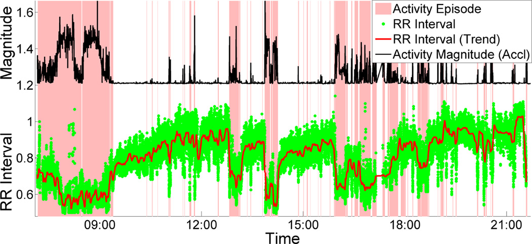
A key weakness of this direct approach for computing the recovery time is that, in the field setting, the HR may take a very long time to recover to the most recent resting HR (see Figure 1), due to confounding factors, such as caffeine intake, during or after the physical activity episode, that typically raise the HR, resulting in a higher resting HR.

Figure 1.

ECG RR interval decreases due to activity which recovers exponentially during stationary period.

Model Based Approach

To address this weakness, we developed an alternate, model-based approach, which learns a participant-specific HR recovery rate that can be used to estimate the time during which the heart-rate should recover, given the most recent peak heart-rate during physical activity and resting heart-rate before physical activity. An additional benefit of the model is that it summarizes the data succinctly in one parameter. Finally, computation of the recovery rate in the natural environment could serve as an indicator of cardiovascular fitness, similar to the 6-minute walk tests [56] done in clinics.

Estimation of Recovery Rate

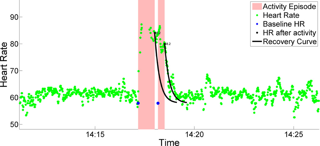
According to [23, 33], heart-rate after an arousal (e.g., activity) recovers exponentially (see equation (1)). Figure 2, which plots one participant’s heart-rate during a physical activity episode, illustrates this exponential recovery. In equation (1), HR_Rest is the resting heart-rate before the physical activity episode, HR_Peak is end-of-activity heart rate at time t₀, and HRR is heart rate during the recovery period at time t. The constant τ represents the exponential recovery rate. Whilst there is a possibility that it can vary across time, our model makes a simplifying assumption of a constant participant-specific recovery rate.

Figure 2.

Heart-rate increases due to activity. Exponential recovery parameter τ is learnt for each participant. 99% exponential recovery curve (equation 1) is shown. Before the heart rate is recovered another activity happened. So baseline heart rate is carry forwarded.

After we have learned the recovery rate for a particular participant, we can use equation (2) to estimate the recovery duration once physical activity is over.

$$HRR=H{R}_{\mathit{\text{Rest}}}+(H{R}_{\mathit{\text{Peak}}}-H{R}_{\mathit{\text{Rest}}})e^{-\frac{t-t_0}{\tau }}$$ (1)

$$t-t_0=\tau \text{ ln}\frac{H{R}_{\mathit{\text{Peak}}}-H{R}_{\mathit{\text{Rest}}}}{HRR-H{R}_{\mathit{\text{Rest}}}}$$ (2)

To learn the recovery rate parameter τ for each participant, we first identify and isolate clean episodes where there is at least a 2-minute rest period (detected by accelerometry), needed to compute HR_Rest, followed by an activity period of at least 2 minutes to represent a significant activity episode, and lastly at least a 2-minute stationary period so we can compute the latency to recover. Next, for each such episode, we derive HR_Rest as the median HR of the last one minute of the initial rest period, and HR_Peak as the median HR of the last 10 seconds of the activity period. Finally, we compute the times required for the HR to drop 10%, 20%, up to 90% of the total increase in HR from rest to peak — [HR_Peak − HR_Rest]. With these quantities defined for all episodes, equation (2) can be used to learn τ using least-squares regression.

We computed the recovery rate τ for each participant. The mean of recovery rates across all 38 participants τ̄ is 19.8 seconds (SD=6.3). Participants’ mean 95% recovery duration of 59.3 seconds (SD=18.9), is consistent with the literature [20].

Isolating and Excluding Activity Confounds

Figure 2 shows an example of the effect of activity on heart rate in daily life. For any such activity episode, we compute HR_Rest and HR_Peak. Then, we use equation (2) and the learned value of τ to estimate the time interval (t − t₀) required for the heart-rate to return to resting heart-rate. Rather than requiring HRR to return to HR_Rest exactly, we consider the heart-rate that has dropped down to the line HR_Rest + σ_HR as fully recovered, where σ_HR is the standard deviation of all heart-rates during stationary intervals. Adding σ_HR to HR_Rest allows for any natural variations in the resting heart-rate throughout the day.

Using this model, in addition to the entire physical activity interval, the estimated recovery interval (t − t₀) that follows is excluded from analysis, i.e., considered missing for the purpose of stress inferencing. With this approach, only 7.4% of data (as opposed to 35%) are excluded due to recovery from physical activity, in addition to 22.7% that are directly affected by physical activity (for a total of 30.1% of all data).

MISSING DATA IMPUTATION

Standard methods for finding trends in time-series data [3, 8] require continuous data streams. To apply these methods, we needed a method to impute the missing data. Missing data in time series of stress assessments can be due to unavailability of data or due to presence of confounder such as physical activity. Before imputation, we need to rule out the possibility that the data are Missing Not At Random (MNAR) [17]. We use the self-report item “Nervous/Stressed?” (Likert 1–6) to check the assumption of independence. To address participant biases, we use the z-score of self-report responses. We find no significant difference in self-reported stress during stationary moments and moments of physical activity (p = 0.984 on Wilcoxon signed-rank test, paired two-tail, n = 31). We also find no significant difference in self-reported stress between stationary and missing data periods (p = 0.841 on Wilcoxon signed-rank test, paired two-tail, n = 24). Therefore, we conclude that our missing data in stress assessments are not MNAR. They can be either Missing Completely At Random (MCAR) or Missing At Random (MAR) [17].

We believe that our missing data should be considered Missing At Random (MAR) [10] because stress can be explained by other known contextual variables [21, 24, 54] such as day of the week, time of day, previous stress levels, and the slope and intercept of previous time-series samples. We use these variables to impute the missing data using the K-Nearest Neighbor method proposed in [27, 60, 63].

We note that although we impute missing data to have a continuous time-series of stress assessments, we programmed our JITI model so that it provides an intervention only when there are non-imputed sensor-inference data (data-loss <50%) with no confounding physical activity.

FIELD VALIDATION OF STRESS ASSESSMENT

The previously-described cStress model captures the instantaneous physiological response to stress. Although this model was validated in both lab and field settings [34], before using it on our dataset obtained from polydrug users, we validate it against their field self-reports. We use the same approach described in [34] to map cStress output to self-report ratings.

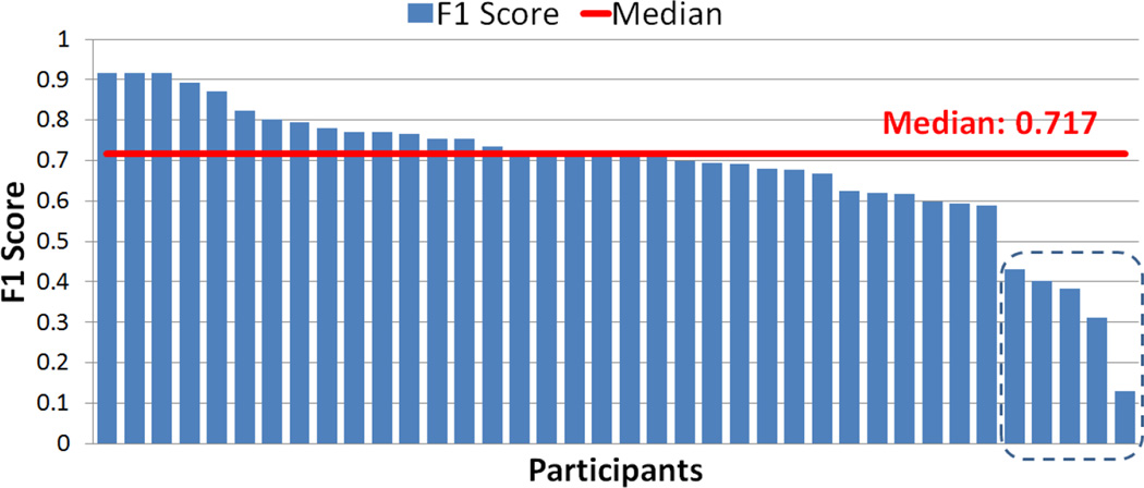
Figure 3 summarize the F1 scores across participants. They range from 0.130 to 0.917 with a median of 0.717. Although the F1 scores are acceptable for majority of the participants, there are 5 participants whose low F1 score seem to suggest poor agreement between self-reported stress and the model output. This observation has lead us to analyze the consistency of their self-reports, because they may be subject to consistent bias or careless responding.

Figure 3.

F1 score between self-report and sensor assessment range from 0.130 to 0.917 with median 0.717. Bottom 5 have unacceptable self-report consistency score with median cronbach’s alpha score 0.335 while overall consistency score is 0.843.

We use Cronbach’s alpha [5] to assess the consistency of the self-reported responses. Cronbach’s alpha measures the internal consistency of items that measures the same psychological construct. In most studies, an alpha score of 0.7 or higher is regarded as acceptable [5].

We compute the Cronbach’s alpha using 5 affect items of self-report — “Cheerful?”, “Happy?”, “Frustrated/Angry?”, “Nervous/Stressed?”, and “Sad?” (The two positive items, “Cheerful?” and “Happy?”, were reverse-coded). The overall consistency score across of all participant’s self-reports is 0.843. We compute Cronbach’s alpha for the 5 participants from Figure 3 who show poor F1 score. They have unacceptable self-report consistency scores with a median Cronbach’s alpha of 0.335. Furthermore, the participant with the smallest F1 score (0.13) answered “3” on item “Nervous/Stressed?” in 173 out of 177 self-reports, suggesting a bias toward neutral self-assessment. These observations also demonstrate the value of an objective sensor-based model of stress.

The above test not only demonstrated the validity of the cStress model in our independent data set, but it also shows the effectiveness of the imputation process since this validation was done on the imputed time series.

LOCATING STRESSFUL EPISODES

There are two types of JITIs. Proactive JITIs are intended to precede and prevent an adverse event, such as an escalation of moderate stress to severe stress. Reactive JITIs follow an adverse event and are intended to mitigate its effects. Although we did not implement a JITI in the current project, we developed our assessment methods with that goal in mind. For either type of JITI, we need a method to determine from a time series of stress data whether a significant stress episode is occurring and if so, when it starts and ends.

To find significant stress episodes in our rapidly varying time-series data, we adapt a stock-prediction model. Such a model operates on a similar dataset, where there exist time-series of stock prices and the objective is to predict the precise moments of buy or sell events, based on prior observations. Methods such as the Relative Strength Index (RSI) [64] and Bollinger Band [6] estimate whether stock is in an oversold or overbought condition and provide a buy or sell signal, respectively. “Oversold” means there are fewer people who can sell the stock relative to the number wishing to buy, indicating that the stock is undervalued and will eventually increase in price. The reverse is true for stocks that are overbought.

However, the assumptions that apply to stock prices do not hold for stress levels. If someone is extremely relaxed it does not imply that his/her stress level will go up as a consequence. Fortunately, this assumption is not built into the method we use, called Moving Average Convergence Divergence (MACD) [3], which has recently been used to detect trends in physiological data [33]. MACD estimates the trend based on short-term and long-term Exponential Moving Average (EMA). It provides one signal when the trend is going up and another signal when it is going down. When applied on the stress likelihood time-series, MACD can provide a signal for a proactive intervention when the stress likelihood is going up and a reactive intervention when the stress likelihood is going down.

MACD is computed as follows:

$$M=EMA(L;w_{\mathit{\text{slow}}})-EMA(L;w_{\mathit{\text{fast}}})$$ (3)

$$S=EMA(M;w_{\mathit{\text{signal}}}),$$

where L is the stress likelihood time-series, M is the so-called MACD line, and S is the so-called MACD Signal Line. As the formula shows, M is calculated by subtracting a fast-moving, short-term EMA line from a slow-moving, long-term EMA line. The intersection of M and S indicates a change in trend, and the sign of the difference between M and S indicates whether the trend is positive or negative.

Before applying MACD, it is important to address the fact that the stress likelihood time-series is rapidly varying and that it may contain inaccuracies as it is the output of a machine learning model that is rarely perfect. To account for this, we first smooth the stress likelihood time-series using a simple moving average with a 2 minute window length, a duration we selected based on visual inspection.

We tune the window length parameters, w_slow, w_fast, and w_signal, used in (3), seeking to maximize $\frac{\mathit{\text{gain}}}{N}$, where gain is defined as the total area under the stress likelihood time-series curve during positive-trend intervals, whereby the start and end of each positive-trend interval are dictated by the MACD rule, mentioned above, and N is the number of positive-trend intervals. Dividing by N discourages window lengths that result in a very large number of short positive-trend intervals. Using a grid search with progressive zoom, with initial grids covering the range from 5 seconds to 30 minutes for each parameter, we found that the optimal window lengths are: w_slow = 7.5 minutes, w_fast = 1.67 minutes, and w_signal = 14.2 minutes, respectively.

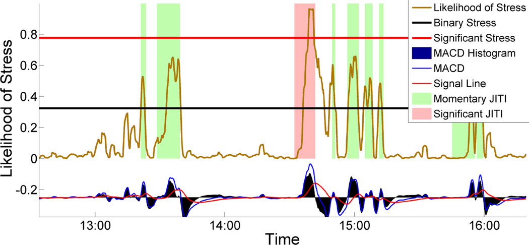
Figure 4 shows a typical example of stress likelihood time-series, with colored boxes highlighting the positive-trend intervals, chosen by the MACD rule using the optimal window length parameters. As the figure illustrates, this approach is able to detect starts for good-quality positive-trend intervals in stress likelihood time-series. Additionally, we show that stress densities for the minute after the detected positive-trend interval starts are significantly greater than those for the preceding minute (p < 0.001 on Wilcoxon signed-rank test, paired one-tail, n = 15, 434). As an added bonus, we can use the MACD rule to comprehensively mark the start and end of each stress episode, defined as the interval containing a positive-trend interval and an immediately following negative-trend interval.

Figure 4.

Timing of just-in-time stress intervention for momentary and significant stress episode. Starting of a rectangular region indicates precise proactive intervention timings generated by MACD.

Defining Significant and Momentary Stress Episode

We define two types of stress episodes: Significant Stress Episode (SSE) and Momentary Stress Episode (MSE). MACD divides the stress-likelihood time-series into smaller variable length, increasing and decreasing episodes. An episode in the time-series is defined as an increasing trend, immediately followed by a decreasing trend. There are 15,434 such episodes. However, in some episodes, stress-likelihood does not cross the binary stress classification threshold (from cStress). Such instances are discarded, leaving 9,087 episodes for further analysis. Significant stress episodes are those that have a high likelihood of stress and persist for a significant duration. All others are momentary.

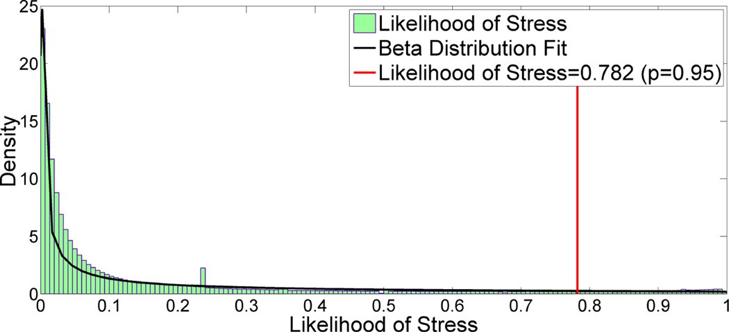
To decide which stress likelihoods are significantly high, we calculate a stress-likelihood threshold ν based on the 95^th percentile of stress-likelihood values. To address the between-participant differences, we calculate participant-specific thresholds, based on each participant’s stress likelihoods only. All stress episodes with likelihoods above this threshold are marked as SSE candidates.

Figure 5 is a histogram of all stress likelihoods pooled together. As it shows, the stress likelihoods are skewed to the left and follow the Beta distribution with parameter estimates α = 0.222 and β = 1.027. We had sufficient data for every participant, from which ν’s could be easily found. If sufficient data are not available for a participant (e.g., when a participant has just begin providing data), we can compute ν based on the estimated parameters of the Beta distribution. In particular, the likelihood threshold ν can be calculated using the inverse Beta Cumulative Distribution Function (CDF), $F_{\mathit{\text{Beta}}}^{-1}(p=0.95|\alpha =0.222,\beta =1.027)$.

Figure 5.

The likelihood of stress follow beta distribution with shape parameter α = 0.222 and β = 1.027. Significant stress threshold is 0.782 (p=0.95).

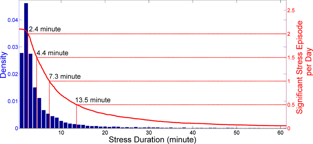
Figure 6 illustrates how duration threshold, λ, informs the selection process for SSE candidates. We first select the desired number of significant stress episodes per day, d, and then, we can simply select the λ that corresponds to d episodes per day. The durations of SSE candidates follow the LogNormal distribution, with estimated parameters μ = 2.064 and σ = 0.871. Out of 9,087 stress episodes, 2,082 contains high stress likelihood (2.1/day). Researchers who are in the designing phase of a stress intervention with no access to data, can calculate λ using the following formula: E(SSE/day) = (1 − F_logNorm (λ|μ = 2.064, σ = 0.871))* 2.1, where F_logNorm(d|μ, σ) is the LogNormal CDF.

Figure 6.

Stress episode with high likelihood of stress (95th percentile) (see figure 5) and a duration of more than duration threshold is marked as a significant stress episode. For a duration threshold 7.3 minute leads to one expected significant stressful episode per day (10+ hours of sensor wearing time).

The rule for identifying the SSEs is as follows — all those stress episodes that have stress likelihoods greater than the threshold of ν and persist for duration greater than λ. We identify other stress episodes as MSEs. Figure 4 shows several examples of SSEs and MSEs.

Table 1 summarizes descriptive statistics for SSEs and MSEs. In total, there are 9,087 stress episodes, with an expected daily frequency of 9.2. A duration threshold of 13.5 minutes labels 498 (or 0.5/day) as significant stress episodes.

Table 1.

In total there are 9,087 stress episodes with an expected count per day of 9.2. A duration threshold of 13.5 minutes labels 498 significant stress episodes, with an expected daily count 0.5.

Significant Stress Episode			Momentary Stress Episode
Duration (minute)	Total Count	E(count) per day	Total Count	E(count) per day
13.5	498	0.5	8,589	8.7
7.3	997	1.0	8,090	8.2
2.4	1,992	2.0	7,095	7.2

APPLICATIONS OF OUR MODEL

To demonstrate the utility of our model, we analyze the relationship between successive stress episodes and the variabilities in stress episodes across persons and situations, time of day, physical activity, and location. Finally, we investigate the feasibility of predicting the onset of a significant episode upon observing a rapid rise in stress.

Role of Prior Stress

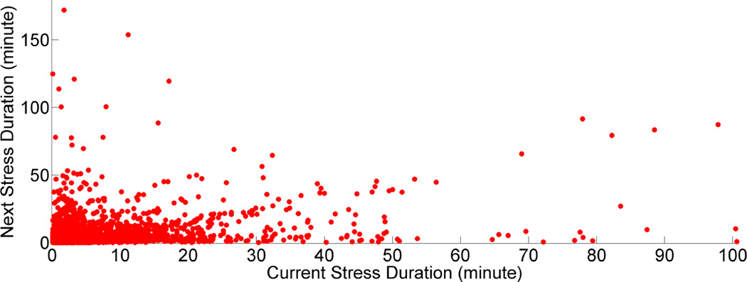
We analyze the relationship between durations of successive stress episodes. Figure 7 is a scatter plot of the duration of the current stress episode versus the duration of the preceding stress episode. We observe a healthy correlation of 0.42. This correlation can be explained by theory and evidence [30, 31, 50] suggesting a spiral process where current exposure to stressors can lead to subsequent reactivity to other stressors by attenuating the state coping capability of the person. For example, stressors such as facing financial troubles may decrease the person’s stress coping capacity. This may lead the person to respond with subsequent stress to an event or an environment that would, in other circumstances, be easy to deal with, such as being in a noisy environment.

Figure 7.

Next stress duration as a function of current stress duration. Surprisingly, the correlation observed here is 0.4243.

Need for Personalization

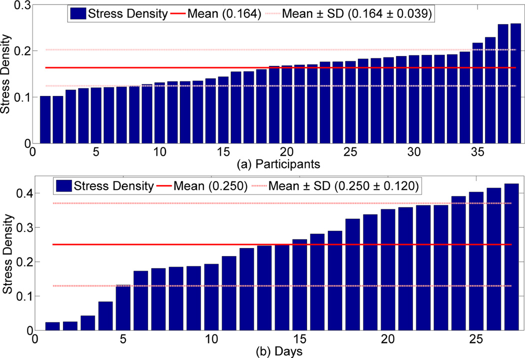
We next analyze the variability in stress densities across participants and across days for the same participant. Figure 8(a) shows the stress density for each participant in increasing order. There is wide between-person variation. The two most stressed participants are twice as stressed, on average, as the two least stressed participants. Figure 8(b) shows daily stress for the participant with maximum overall stress density. Here, for 4 (out of 27) days, that participant had three times lower stress density than he/she had on average. On the other hand, the most stressful day has a stress density twice the overall average. These observations demonstrate that the frequency (or even the content) of stress interventions may need to be calibrated to each person and for each day.

Figure 8.

(a) Overall participants stress. We observe that there exist wide between person variation. (b) Day wise stress for the participant with maximum stress density. We observe that there exist wide between day variation.

Temporal Effect on Stress

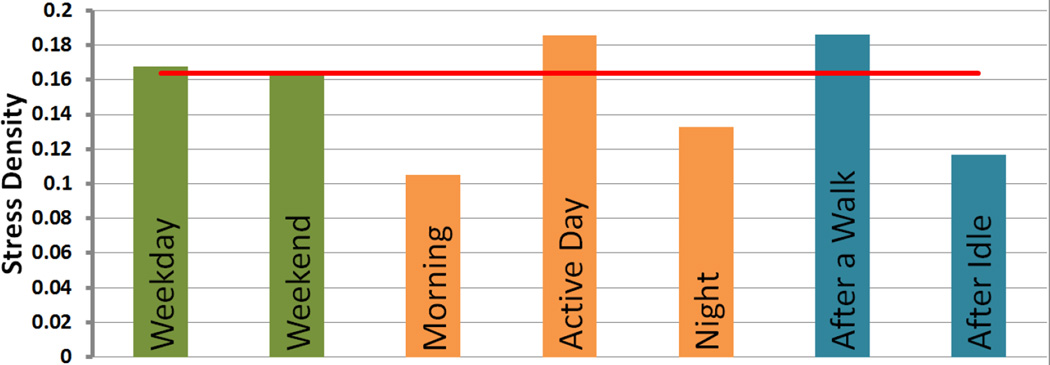
We do not observe any significant difference in stress level between weekdays and weekends (0.168 vs. 0.163, p = 0.744 on Wilcoxon signed-rank test, paired two-tail, n = 38). Most of our participants did not have full-time jobs; this may explain the absence of a difference.

As hypothesized in [39], we observe that in our sample, stress varies by time of day. It is low in the mornings, rises during the middle portion of the day, and subsides again at night. These differences were significant in pairwise comparisons of midday versus morning (0.186 vs. 0.105, p < 0.001 on Wilcoxon signed-rank test, one-tail, n = 38) and midday versus night (0.186 vs. 0.133, p = 0.001 on Wilcoxon signed-rank test, one-tail, n = 38), and not morning versus night (0.105 vs. 0.133, p = 0.055 on Wilcoxon signed-rank test, one-tail, n = 38). These are expected observations, as the active day is likely spent looking for work and drugs and being exposed to drug cues and potential conflicts. Some of these events may occur during evening and night times as well, but are less likely than during the daytime.

Effect of Activity on Stress

Even after we remove the confounding periods of moderate to high physical activity, we still find that stress density for the next 15 minutes after a walk is higher than usual, as shown in Figure 9. In contrast, stress density was lower in the 60 minutes following a 60 minutes of inactivity, (which generally happen at home) (0.186 vs. 0.117, p = 0.001 on Wilcoxon signed-rank test, paired one-tail, n = 38).

Figure 9.

Role of temporal and activity on stress density. Here morning is defined as before 8 AM, day time as 8 AM to 7 PM, and night as after 7 PM. Red line represents the overall stress density.

This observation seems to contradict the common belief that physical activity such as walking helps to reduce stress [15]. This apparent contradiction could be because our participants’ physical activities usually corresponds to transportation (e.g., walking and public transport). Upon conclusion of these episodes, they could have been exposed to cues, unpleasant environments, work challenges, etc. They could also have been engaged in jobs that required significant physical activity. This observation prompted us to investigate the role of environmental context in stress.

Environmental Effect on Stress

To analyze the effect of environment on stress, we use the Neighborhood Inventory for Environmental Typology (NIfETy) [25] as a measure of environmental disorder. GPS data is mapped to this index. The collection of NIfETy data has occurred in several waves, starting in 2005. We use data from Wave Eight, because they were collected close in time to our participants’ provision of GPS data. During Wave Eight, trained NIfETy raters sampled 528 individual georeferenced blockfaces in the city where the study was conducted. The raters noted the presence or absence of each of 77 variables, which were divided a priori into five categories: (1) Social Disorder, (2) Physical Disorder, (3) Drug Paraphernalia, (4) Adult Activity, and (5) Youth Activity.

Method

To estimate probable NIfETy ratings for the areas between the 528 rated city blockfaces, we develop a model that incorporated data from remote-sensing-derived maps of surface imperviousness and landcover [65]. The remote-sensing data consist of 180,000 pixel values measured as an image across the city. Next, we use a distance matrix to measure the distance between all NIfETy blockfaces and the centroid coordinate location for individual pixels in the remote sensing image of the city. We complete the distance measurements iteratively, where the first matrix is the distance from each of the 180,000 pixels to the closest NIfETy blockface. The second iteration is the distance from each pixel to second-closest NIfETy blockface. This process is replicated with the distance matrix for all 528 NIfETy blockfaces, so that we have 528 distance layers for each of the 180,000 pixels. These layers are then rasterized for the city and sampled for each NIfETy location.

Next, we develop a RandomForest based classifier [7] to predict a dichotomous outcome (i.e., 0 = “absent” or 1 = “present”) for each of the 77 NIfETy variables, using the 2 remote sensing layers, coordinate location, and the 528 distance values. We reason that with the distance values included, the machine-learning model would generate predictions similar to those of Kriging, a common geospatial interpolation method that uses distance alone to make its predictions [18]. By adding remote-sensing data to our model, we account for real-world physical environments in the city.

We then generate a citywide map of inferred probabilities for each of the 77 NIfETy variables at each pixel. We use Cohen’s kappa to compare model-inferred probabilities to actual ratings at the NifETy blockfaces (representing a gold standard). Only NIfETy values with a kappa greater than 0.4 are used in our analysis here (n=61) as predictors of stress ratings. The posterior probability computed by the Random Forest model is used to infer the binary labels: “absent”/“present”, using 0.5 as the binary threshold.

Findings

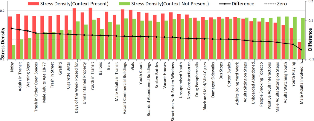
Figure 10 presents the stress densities across 37 different location contexts, for which the classification κ > 0.7, distinguishes between cases where the context is present and absent. We observe that noisy location; presence of graffiti, cigarette butts, trash in street, and bars are associated with high stress likelihood. Bars may be a potent cue for drugs and hence may elevate stress in our population. In contrast, locations where the NIfETy raters had seen male adults involved in positive interaction and youth playing are associated with lower stress than average.

Figure 10.

Effect on stress density across different location contexts detected with κ > 0.7. Noisy environment is highly associated with stress.

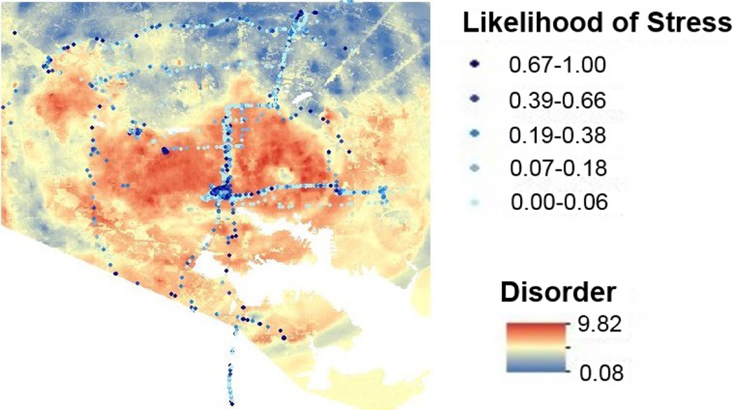
This suggests that geolocation tracking can help inform the timing of JITIs, that might, for example, propose a relatively less stressful route. As an example, Figure 11 shows one participant’s stress assessments overlaid on disorder map of the city. Disorder here is the aggregated posterior probability value for the top 10 NIfETy variables with κ > 0.70. The figure suggests that people are more likely to be stressed in some specific parts of the city with high disorder score.

Figure 11.

The likelihood of stress for one participant overlaid on the disorder map. Disorder here is the aggregated posterior probability value for top 10 NIfETy variables (see figure 10) with κ > 0:70.

Prediction for Proactive Stress Intervention

As another application of our model, we employ it to train a classifier for predicting significant stress episodes. As described earlier, we use the MACD method to identify and locate stress episodes. All stress episodes, momentary or significant, are considered candidate windows during the training process. Our goal in this prediction task is to determine early on, as soon as an MSE is detected, whether it will become an SSE, which essentially becomes a MSE/SSE classification task. For this task, we identify and compute 173 candidate features, and then train a model with 100 selected features.

Feature Computation

We compute 173 features to train a MSE/SSE classifier. These features are based on the observations and findings presented earlier.

Time and Day (3 features)

As shown in Figure 9, there are temporal factors that affect stress, such as time of day. Therefore, we include the following features: “time of day,” “hour of day,” and “weekday”.

Previous Stress Episode (3 features)

As shown in Figure 7, durations of adjacent stress episodes are correlated. Hence, we include the features “duration of previous stress episode,” “time since previous episode,” and “time required to cross binary stress threshold.”

Slope and Intercept (22 features)

We use the slope and intercept of a best-fit line, fitted to past stress likelihood values. The rationale behind the inclusion of this feature was an assumption of a “calm before the storm.” In addition, a fast ramp-up of the stress likelihood has a good potential to break into an SSE. To compute these features, we use the slope and intercept associated with the crossing of the binary stress threshold. We also use the slope and intercept of prior 30 sec, 1 min, 2 min, etc., up to 10 min.

Prior Stress Density and Skewness (30+30 features)

Figure 7 suggests that the prior stress density is correlated with the current stress density. Hence, we compute the stress densities of the previous N minutes, where N increases from 1 to 30. We also compute the skewness of the previous N minutes, varying N from 1 to 30.

Location (61 features)

Figure 10 shows the apparent effect of location on stress density. We use 61 NIfETy scores out of 77 which are detected with performance κ > 0.4.

Physical Activity (24 features)

Figure 9 shows that there is a significant association between the post-walk period and a high stress likelihood. Inspired by [58], we use 24 aggregated features of activity (All-N, Any-N, Duration-N, and Change-N) over windows of varying size N — 5 min, 10 min, 15 min, 20 min, 25 min, and 30 min.

Feature Selection

To improve the generalization performance of the classifier, we perform feature selection and retain only the top 100 features with the highest information gain [13]. This ensure approximately one feature for every 100 samples (total 9,087 samples).

Model

We train a RandomForest learning algorithm [7] to discriminate between MSEs and SSEs. To address the issue of imbalanced class sizes, we use a cost-sensitive classification approach [16], assigning a higher cost to misclassifications of actual SSEs. For evaluation, we use leave-one-subject-out validation.

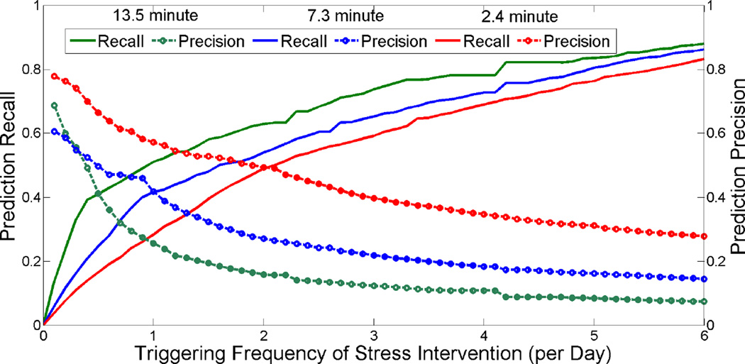
Table 2 summarizes the performance of our model. The model is able to predict SSEs with a duration of 13.5 minutes with accuracy of 94.8% and κ = 0.444. Figure 12 shows the tradeoff analysis. The x-axis represents a triggering frequency of stress intervention per day and the two y-axes represent precision and recall for predicting SSEs. Researchers designing an intervention can use this information to find a triggering frequency that will achieve specific values of precision and recall.

Table 2.

Performance of the prediction of Significant Stress Episodes with duration 13.5, 7.3, and 2.4 minute.

Duration (minute)	E(count) per day	Accuracy	Kappa
13.5	0.5	94.8%	0.444
7.3	1.0	88.3%	0.428
2.4	2.0	77.7%	0.495

Figure 12.

Tradeoff analysis for triggering frequency of stress intervention. The x-axis represents model proposed triggering frequency of stress intervention per day and two y-axes represent precision and recall for predicting SSEs.

DISCUSSION, LIMITATIONS, AND FUTURE WORK

Our work has several limitations. First, physiological indices of stress can be confounded by pharmacological factors, such as smoking, coffee intake, or other drugs. Automated detection of those events could help further refine stress inferences.

Second, we assume that the recovery rate is constant for a participant, but, in reality the rate may change over the course of a day or context (e.g., caffeine intake). Calibrating the recovery rate to time of day or to contexts (e.g., smoking, drinking, etc.) represents interesting future work opportunities.

Third, our model for generating stress intervention triggers can be supplemented with visual-exposure (via smart eyeglasses), digital traces (e.g., appointments on a smartphone calendar), and social exposures (e.g., twitter, facebook, etc.) to improves its accuracy and context sensitivity.

Fourth, our dataset was collected from a specific population from a specific location, whose lapses due to stress might lead to devastating consequences. Therefore, the findings and their implications may differ with other populations. Nevertheless, we present a method together with its feasibility and applicability that can potentially be carried over to other populations and locations.

Finally, our work demonstrates only the mechanism for determining when to intervene. It does not directly provide an efficacious intervention, which requires making choices on not only the timing of delivery, but also the right content, the adaptation mechanisms for personalizing it to the individual and the user’s context, and selecting the right modality for delivery (e.g., on the phone, on a smart watch). Conducting a micro-randomized trial [49] could be a natural next step to determine the most efficacious strategy for personalized JITIs. Several populations can be targeted for stress JITI where stress plays a significant role. They include those with problems of addiction, migraine, panic disorders, depression, etc.

CONCLUSION

Just-in-time interventions have been possible for quite some time for applications such as traffic-aware navigation. GPS sensors have also made it possible to explore interventions that are based on geofencing. Our work presents the first approach to analyze the time-series of stress data for determining the timing of just-in-time stress intervention. Given the wide prevalence of stress and its adverse impacts on health, job performance, and quality of life, stress management is useful for everyone. This work opens up numerous opportunities to now design efficacious interventions for helping dealing with daily stress in work life, social life, or otherwise. For the specific population addressed here — outpatients undergoing treatment for addiction-stress management in real-world circumstances will be most valuable if it is linked to prevention of drug craving and relapse.

In addition to showing how time-series data can be mined for determining the timing of interventions, our work makes several methodological contributions. For example, our method of estimating the recovery time of physiology from a physical activity episode could possibly be used as a measure of cardiovascular fitness outside of controlled settings for heart patients. Our work also proposes a method to mine time series sensor data on human health status and explore the tradeoffs between intervention frequency and probability of capturing the event of interest. This approach can be adopted to analysis of other sensor data that may help determine the best timing and frequency for mHealth interventions in daily life.

REFERENCES

- 1.ANT Radio. [Accessed: January 2016]; http://www.thisisant.com/ [Google Scholar]
- 2.Abbott H, Powell D. Land-vehicle navigation using gps. Proceedings of the IEEE. 1999;87(1):145–162. [Google Scholar]
- 3.Appel G. Technical analysis: power tools for active investors. FT Press; 2005. [Google Scholar]
- 4.Aswani A, Tomlin C. American Control Conference (ACC) IEEE; 2011. Game-theoretic routing of gps-assisted vehicles for energy efficiency; pp. 3375–3380. [Google Scholar]
- 5.Bland J, Altman D. Statistics: notes cronbach’s alpha. BMJ. 1997;314(7080):572–572. doi: 10.1136/bmj.314.7080.572. [DOI] [PMC free article] [PubMed] [Google Scholar]
- 6.Bollinger J. Bollinger on bollinger band [Google Scholar]
- 7.Breiman L. Random forests. Machine learning. 2001;45(1):5–32. [Google Scholar]
- 8.Brown R. Smoothing, forecasting and prediction of discrete time series. Courier Corporation; 2004. [Google Scholar]
- 9.Carroll E, Czerwinski M, Roseway A, Kapoor A, Johns P, Rowan K, Schraefel M. Food and mood: Just-in-time support for emotional eating. IEEE ACII. 2013:252–257. [Google Scholar]
- 10.Chandola T, Brunner E, Marmot M. Chronic stress at work and the metabolic syndrome: prospective study. Bmj. 2006;332(7540):521–525. doi: 10.1136/bmj.38693.435301.80. [DOI] [PMC free article] [PubMed] [Google Scholar]
- 11.Choudhary AK, Harding JA, Tiwari MK. Data mining in manufacturing: a review based on the kind of knowledge. Journal of Intelligent Manufacturing. 2009;20(5):501–521. [Google Scholar]
- 12.Chrousos G, Gold P. The concepts of stress and stress system disorders: overview of physical and behavioral homeostasis. JAMA. 1992;267(9):1244. [PubMed] [Google Scholar]
- 13.Cover TM, Thomas JA. Elements of information theory. John Wiley & Sons; 2012. [Google Scholar]
- 14.Davis F, Roseway A, Carroll E, Czerwinski M. Actuating mood: design of the textile mirror; International Conference on Tangible, Embedded and Embodied Interaction; 2013. pp. 99–106. [Google Scholar]
- 15.Davis M, Eshelman E, McKay M. The relaxation and stress reduction workbook. New Harbinger Publications; 2008. [Google Scholar]
- 16.Domingos P. Metacost: A general method for making classifiers cost-sensitive. ACM KDD. 1999:155–164. [Google Scholar]
- 17.Donders A, van der Heijden G, Stijnen T, Moons K. Review: a gentle introduction to imputation of missing values. Journal of clinical epidemiology. 2006;59(10):1087–1091. doi: 10.1016/j.jclinepi.2006.01.014. [DOI] [PubMed] [Google Scholar]
- 18.Epstein D, Tyburski M, Craig I, Phillips K, Jobes M, Vahabzadeh M, Mezghanni M, Lin J, Furr-Holden D, Preston K. Real-time tracking of neighborhood surroundings and mood in urban drug misusers: application of a new method to study behavior in its geographical context. Drug and alcohol dependence. 2014;134:22–29. doi: 10.1016/j.drugalcdep.2013.09.007. [DOI] [PMC free article] [PubMed] [Google Scholar]
- 19.Ertin E, Stohs N, Kumar S, Raij A, al’Absi M, Shah S. Autosense: Unobtrusively wearable sensor suite for inferring the onset, causality, and consequences of stress in the field. ACM SenSys. 2011:274–287. [Google Scholar]
- 20.Esco M, Olson M, Williford H, Blessing D, Shannon D, Grandjean P. The relationship between resting heart rate variability and heart rate recovery. Clinical Autonomic Research. 2010;20(1):33–38. doi: 10.1007/s10286-009-0033-2. [DOI] [PubMed] [Google Scholar]
- 21.Evans G, Wener R, Phillips D. The morning rush hour predictability and commuter stress. Environment and Behavior. 2002;34(4):521–530. [Google Scholar]
- 22.Fogarty J, Hudson S, Lai J. Examining the robustness of sensor-based statistical models of human interruptibility. ACM CHI. 2004:207–214. [Google Scholar]
- 23.Freeman J, Dewey F, Hadley D, Myers J, Froelicher V. Autonomic nervous system interaction with the cardiovascular system during exercise. Progress in cardiovascular diseases. 2006;48(5):342–362. doi: 10.1016/j.pcad.2005.11.003. [DOI] [PubMed] [Google Scholar]
- 24.Fritz C, Sonnentag S, Spector P, McInroe J. The weekend matters: Relationships between stress recovery and affective experiences. Journal of Organizational Behavior. 2010;31(8):1137–1162. [Google Scholar]
- 25.Furr-Holden D, Smart M, Pokorni J, Ialongo N, Leaf P, Holder H, Anthony J. The nifety method for environmental assessment of neighborhood-level indicators of violence, alcohol, and other drug exposure. Prevention Science. 2008;9(4):245–255. doi: 10.1007/s11121-008-0107-8. [DOI] [PMC free article] [PubMed] [Google Scholar]
- 26.Han T, Xiao X, Shi L, Canny J, Wang J. Balancing accuracy and fun: Designing camera based mobile games for implicit heart rate monitoring. ACM CHI. 2015:847–856. [Google Scholar]
- 27.Hastie T, Tibshirani R, Sherlock G, Eisen M, Brown P, Botstein D. Imputing missing data for gene expression arrays. 1999 [Google Scholar]
- 28.Hernandez J, Paredes P, Roseway A, Czerwinski M. Under pressure: sensing stress of computer users. ACM CHI. 2014:51–60. [Google Scholar]
- 29.Hirshfield LM, Solovey ET, Girouard A, Kebinger J, Jacob RJ, Sassaroli A, Fantini S. ACM CHI. ACM; 2009. Brain measurement for usability testing and adaptive interfaces: an example of uncovering syntactic workload with functional near infrared spectroscopy; pp. 2185–2194. [Google Scholar]
- 30.Hobfoll SE. Conservation of resources: A new attempt at conceptualizing stress. American psychologist. 1989;44(3):513. doi: 10.1037//0003-066x.44.3.513. [DOI] [PubMed] [Google Scholar]
- 31.Hobfoll SE, Vinokur AD, Pierce PF, Lewandowski-Romps L. The combined stress of family life, work, and war in air force men and women: A test of conservation of resources theory. International Journal of Stress Management. 2012;19(3):217. [Google Scholar]
- 32.Hong J, Ramos J, Dey A. Understanding physiological responses to stressors during physical activity. ACM UbiComp. 2012:270–279. [Google Scholar]
- 33.Hossain S, Ali A, Rahman M, Ertin E, Epstein D, Kennedy A, Preston K, Umbricht A, Chen Y, Kumar S. Identifying drug (cocaine) intake events from acute physiological response in the presence of free-living physical activity. ACM IPSN. 2014:71–82. [PMC free article] [PubMed] [Google Scholar]
- 34.Hovsepian K, al’Absi M, Ertin E, Kamarck T, Nakajima M, Kumar S. cstress: towards a gold standard for continuous stress assessment in the mobile environment. ACM UbiComp. 2015:493–504. doi: 10.1145/2750858.2807526. [DOI] [PMC free article] [PubMed] [Google Scholar]
- 35.Iqbal S, Zheng X, Bailey B. Task-evoked pupillary response to mental workload in human-computer interaction. ACM CHI Extended Abstracts. 2004:1477–1480. [Google Scholar]
- 36.Iqbal ST, Adamczyk PD, Zheng XS, Bailey BP. Towards an index of opportunity: understanding changes in mental workload during task execution. ACM CHI. 2005:311–320. [Google Scholar]
- 37.Jaimes L, Llofriu M, Raij A. A stress-free life: just-in-time interventions for stress via real-time forecasting and intervention adaptation. ICST BODYNETS. 2014:197–203. [Google Scholar]
- 38.Kapoor A, Horvitz E. Experience sampling for building predictive user models: a comparative study. ACM CHI. 2008:657–666. [Google Scholar]
- 39.Kudielka B, Schommer N, Hellhammer D, Kirschbaum C. Acute hpa axis responses, heart rate, and mood changes to psychosocial stress (tsst) in humans at different times of day. Psychoneuroendocrinology. 2004;29(8):983–992. doi: 10.1016/j.psyneuen.2003.08.009. [DOI] [PubMed] [Google Scholar]
- 40.Lyu Y, Luo X, Zhou J, Yu C, Miao C, Wang T, Shi Y, Kameyama K-i. Measuring photoplethysmogram-based stress-induced vascular response index to assess cognitive load and stress. ACM CHI. 2015:857–866. [Google Scholar]
- 41.MacLean D, Roseway A, Czerwinski M. Moodwings: a wearable biofeedback device for real-time stress intervention. ACM PETRA. 2013:66. [Google Scholar]
- 42.Mark G, Gudith D, Klocke U. The cost of interrupted work: more speed and stress. ACM CHI. 2008:107–110. [Google Scholar]
- 43.Matthews M, Snyder J, Reynolds L, Chien JT, Shih A, Lee JW, Gay G. Real-time representation versus response elicitation in biosensor data. ACM CHI. 2015:605–608. [Google Scholar]
- 44.McDuff D, Karlson A, Kapoor A, Roseway A, Czerwinski M. Affectaura: an intelligent system for emotional memory. ACM CHI. 2012:849–858. [Google Scholar]
- 45.McEwen B. Protection and damage from acute and chronic stress. Ann NY Acad Sci. 2004;1032:1–7. doi: 10.1196/annals.1314.001. [DOI] [PubMed] [Google Scholar]
- 46.McEwen B. Stress, adaptation, and disease: Allostasis and allostatic load. Annals of the New York Academy of Sciences. 2006;840(1):33–44. doi: 10.1111/j.1749-6632.1998.tb09546.x. [DOI] [PubMed] [Google Scholar]
- 47.McEwen B. Physiology and neurobiology of stress and adaptation: Central role of the brain. Physiological Reviews. 2007;87(3):873–904. doi: 10.1152/physrev.00041.2006. [DOI] [PubMed] [Google Scholar]
- 48.McEwen B, Stellar E. Stress and the individual: mechanisms leading to disease. Archives of Internal Medicine. 1993;153(18):2093. [PubMed] [Google Scholar]
- 49.Murphy S. Micro-randomized trials & mhealth. 2014 doi: 10.1002/sim.6847. [DOI] [PMC free article] [PubMed] [Google Scholar]
- 50.Nahum-Shani I, Hekler E, Spruijt-Metz D. Building health behavior models to guide the development of just-in-time adaptive interventions: a pragmatic framework. Health Psychology. doi: 10.1037/hea0000306. [DOI] [PMC free article] [PubMed] [Google Scholar]
- 51.Ni K, Ramanathan N, Chehade M, Balzano L, Nair S, Zahedi S, Kohler E, Pottie G, Hansen M, Srivastava M. Sensor network data fault types. ACM TOSN. 2009;5(3):25. [Google Scholar]
- 52.Plarre K, Raij A, Hossain S, Ali A, Nakajima M, Al’absi M, Ertin E, Kamarck T, Kumar S, Scott M, et al. Continuous inference of psychological stress from sensory measurements collected in the natural environment. IEEE/ACM IPSN. 2011:97–108. [Google Scholar]
- 53.Purpura S, Schwanda V, Williams K, Stubler W, Sengers P. Fit4life: the design of a persuasive technology promoting healthy behavior and ideal weight. ACM CHI. 2011:423–432. [Google Scholar]
- 54.Ragsdale J, Beehr T, Grebner S, Han K. An integrated model of weekday stress and weekend recovery of students. International Journal of Stress Management. 2011;18(2):153. [Google Scholar]
- 55.Rahman M, Bari R, Ali A, Sharmin M, Raij A, Hovsepian K, Hossain S, Ertin E, Kennedy A, Epstein D, Preston K, Jobes M, Beck G, Kedia S, Ward K, alAbsi M, Kumar S. Are we there yet? feasibility of continuous stress assessment via wireless physiological sensors. ACM BCB. 2014:479–488. doi: 10.1145/2649387.2649433. [DOI] [PMC free article] [PubMed] [Google Scholar]
- 56.Rasekaba T, Lee A, Naughton M, Williams T, Holland A. The six-minute walk test: a useful metric for the cardiopulmonary patient. Internal medicine journal. 2009;39(8):495–501. doi: 10.1111/j.1445-5994.2008.01880.x. [DOI] [PubMed] [Google Scholar]
- 57.Sapolsky RM. Why zebras don’t get ulcers: The acclaimed guide to stress, stress-related diseases, and coping-now revised and updated. Macmillan; 2004. [Google Scholar]
- 58.Sarker H, Sharmin M, Ali A, Rahman M, Bari R, Hossain S, Kumar S. Assessing the availability of users to engage in just-in-time intervention in the natural environment. ACM UbiComp. 2014:909–920. doi: 10.1145/2632048.2636082. [DOI] [PMC free article] [PubMed] [Google Scholar]
- 59.Sharmin M, Raij A, Epstien D, Nahum-Shani I, Beck JG, Vhaduri S, Preston K, Kumar S. Visualization of time-series sensor data to inform the design of just-in-time adaptive stress interventions. ACM UbiComp. 2015:505–516. doi: 10.1145/2750858.2807537. [DOI] [PMC free article] [PubMed] [Google Scholar]
- 60.Speed T. Statistical analysis of gene expression microarray data. CRC Press; 2004. [Google Scholar]
- 61.Sun D, Paredes P, Canny J. Moustress: detecting stress from mouse motion. ACM CHI. 2014:61–70. [Google Scholar]
- 62.Tan CSS, Schöning J, Luyten K, Coninx K. Investigating the effects of using biofeedback as visual stress indicator during video-mediated collaboration. ACM CHI. 2014:71–80. [Google Scholar]
- 63.Troyanskaya O, Cantor M, Sherlock G, Brown P, Hastie T, Tibshirani R, Botstein D, Altman R. Missing value estimation methods for dna microarrays. Bioinformatics. 2001;17(6):520–525. doi: 10.1093/bioinformatics/17.6.520. [DOI] [PubMed] [Google Scholar]
- 64.Wilder JW. New concepts in technical trading systems. NC: Trend Research Greensboro; 1978. [Google Scholar]
- 65.Xian G, Homer C. Updating the 2001 national land cover database impervious surface products to 2006 using landsat imagery change detection methods. Remote Sensing of Environment. 2010;114(8):1676–1686. [Google Scholar]