A global distributed basin morphometric dataset

Abstract

Basin morphometry is vital information for relating storms to hydrologic hazards, such as landslides and floods. In this paper we present the first comprehensive global dataset of distributed basin morphometry at 30 arc seconds resolution. The dataset includes nine prime morphometric variables; in addition we present formulas for generating twenty-one additional morphometric variables based on combination of the prime variables. The dataset can aid different applications including studies of land-atmosphere interaction, and modelling of floods and droughts for sustainable water management. The validity of the dataset has been consolidated by successfully repeating the Hack’s law.

Background & Summary

Morphometry, the topographic and bathymetric features of the earth surface, is known as interactions among multiple factors including climate, tectonic, and erosion, and is known to impact landscape, ecology, and consequentially the occurrence and severity of hydro-meteorological hazards. To understand how the natural surface has grown into its current state^1–4, what it will become⁵, and in which way it impacts the environment^6–12, we need distributed geomorphological data at global scale. The most commonly cited geomorphological features, listed in Table 1, were defined nearly 20 years ago, while currently a number of global or regional gridded topographic datasets^13–16 are available to support newly derived geomorphological features.

Table 1. Basin characteristics included in the proposed dataset.

Variable (File Name)	Description	Definition	References
Sμ (SO)	Stream Order(Strahler)	Strahler stream order, numerical measure of river’s branching complexity	28
Nμ (Nu)	Stream Number	order-wise stream segments based on Sμ	29
Lμ (Lu)	Stream Length	order-wise total stream length based on Sμ	29
LMF (MFL)	Maximal Flow Length	the length along the longest watercourse from the mouth to the head of the channel	30
Lv (Lv)	Down Valley Length	The straight distance from the river cell of interest to the basin mouth	30
Lg (Lg)	Length of Overland Flow	The overland flow length to river	29
RB (BR)	Basin Relief	The elevation difference between the highest point on the drainage divide and the mouth	10
LB (BL)	Basin Length	The maximal length of the line from a basin mouth to a point on the perimeter equidistant from the basin mouth in either direction around the perimeter	31
P(P)	Basin Perimeter	The outer boundary of the watershed that enclosed its area	32
Rb	Bifurcation Ratio	Rbμ=Nμ/Nμ+1 (10)	32
BW	Weighted Mean Bifurcation Ratio	${\mathit{B}}_{\mathit{w}}=\frac{1}{{\sum }_1^{\mathit{max}\left({\mathit{S}}_{\mathit{\mu }}\right)-1}\left({\mathit{N}}_{\mathit{\mu }}+{\mathit{N}}_{\mathit{\mu }+1}\right)}\sum _1^{\mathit{max}\left({\mathit{S}}_{\mathit{\mu }}\right)-1}{\mathit{R}}_{b\mathit{\mu }}\left({\mathit{N}}_{\mathit{\mu }}+{\mathit{N}}_{\mathit{\mu }+1}\right)$ (11)	33
Lmμ	Mean Stream Length	Lmμ=Lμ/Nμ (12)	34
Lmrμ	Stream Length Ratio	Lmrμ=Lμ/Lμ-1 (13)	29
Si	Sinuosity Index	Si=LMF/Lv (14)	35
Ff	Form Factor	Ff=A/LB, where A is the drainage area (15)	36
Rr	Relief Ratio	Rr=RB/LB (16)	32
Re	Elongation Ratio	Re=2/LB×(A/π)0.5 (17)	32
Rt	Texture Ratio	Rt=N1/P (18)	29
Rc	Circularity Ratio	Rc=4πA/P2 (19)	37
k	Lemniscate’s value	k=LB2/A (20)	38
Dtμ	Drainage Texture	Dtμ=Nμ/P (21)	29
Dd	Drainage Density	Dd=Lμ/A (22)	31,36
Cc	Compactness Coefficient	Cc=0.2841 P/A0.5 (23)	39
RW	Wandering Ratio	RW=LMF/LB (24)	40
Rf	Fitness Ratio	Rf=LMF/P (25)	41
MB	Basin Magnitude	MB=N1 (26)	10
Fs	Channel Frequency	Fs=Nμ/A (27)	36
Di	Drainage Intensity	Fs/Dd (28)	42
If	Infiltration Number	If=Fs×Dd (29)	42
Rn	Ruggedness Number	Rn=RB×Dd (30)	43

Numerous local geomorphological studies have been conducted using sparse and limited data^{4,6,8,9,17,18}. Only uniform geomorphological features are available for large basins^12,19. Due to the heavy computation of basin delineation and boundary tracing at global scale, some critical features missing from existing datasets are based on boundary information such as basin length and perimeter. A common solution has been to convert those features from easy-to-obtain features (such as drainage area) by means of statistical relations²⁰, which is bound to empirical experience and less accuracy, as will be shown in the Technical Validation Section.

The objective of this paper is to share the first distributed global geomorphological dataset available at 30 arc seconds (denoted as 30’ hereafter) resolution. This dataset groups 30 basin characteristics into two categories, prime (the first 9 variables) and derived (the rest 21 variables) as listed in Table 1. The prime characteristic variables are computed strictly by geomorphic definitions following the from-upstream-to-downstream (FUTD) framework²¹ and using all cells within the basin, while the derived variables are calculated numerically based on the prime variables, therefore they are not archived.

Methods

The dataset is made available by a recently released tool²¹ that can reduce the computation to linear complexity, O(N). Input data used in the morphometric characteristics’ computations include digital elevation model (DEM) flow direction (FDR) and flow accumulation (FAC) maps at 30’ resolution contained in the global shuttle elevation derivatives available at multiple Scales (HydroSHEDS) dataset. The tool is built on a FUTD framework that starts from the most upstream grids (where FAC is equal to 1) and then ‘flows’ to the downstream direction while computing. Redundant computations are avoided by inheriting tributary basin characteristics and eliminating the process of basin delineation and boundary tracing. Through this process, each grid is visited minimal times, which maximizes computation efficiency. For the details of calculating each prime variable in the FUTD framework, a demonstration of the algorithm for a small-scale basin consisting of 44 grids is given at this product’s website, http://engr.uconn.edu/~xshen/GDBC/#example.

Code availability

The matlab codes and user manual of the tool used to generating the dataset are accessible at http://engr.uconn.edu/~xshen/GDBC/software/.

Data Records

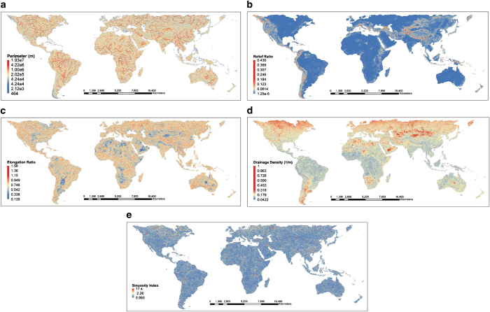
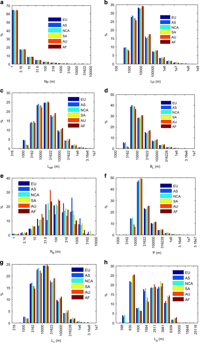
The HydroSHEDS dataset¹³ used in this study can be accessed at http://www.hydrosheds.org. Figure 1 gives snapshot of some selected basin characteristics. In Fig. 1b, large relief ratio appears at mountainous areas including the Alps-Himalaya belt, Cordillera belt, Altai belt, and New Guinea highlands. The probability of basins with high drainage density roughly increases with latitude in both hemispheres. Figure 2 shows the distribution (converted from number of grids to percentage) of prime variables grouped by continent. It shows that distributions of any given prime variable except the basin relief are almost identical among different continents. The significant distinction between basin relief and other prime variables is that the former is a vertical measurement while the latter are all horizontal descriptors.

Figure 1. Selected Geomorphological Variables of the proposed dataset:

(a) perimeter, (b) relief ratio, (c) elongation ratio, (d) drainage density and (e) sinuosity.

Figure 2. Distribution of prime basin characteristics:

(a) Nμ (b) Lμ, (c) L_MF, (d) L_B, (e) R_B, (f) P, (g) L_v, and (h) L_g, grouped by continent: Europe (EU), Asia (AS), North and Central America (NCA), South America (SA), Australia (AU) and Africa (AF). N_μ and L_μ are only displayed for first order streams, i.e., μ=1.

The nine prime variables are can be accessed at figshare via https://figshare.com/s/6cd00491b850bad716d7 (Data Citation 1). Files are stored in GeoTiff format and are projected in world geodetic system 1984 (WGS84). Basin characteristics are compressed into a single file for each continent. An example file name is ‘AF.zip’ with AF standing for Africa. The rest continents are AS for Asia, EU for Europe, AU for Australia, CA for Central America, NA for North America and SA for South America. One will find the file, ‘AF_BL.tif’, among other characteristics by decompressing the ‘AF.zip’ file. Other variable abbreviations include BR, Lg, Nu, Lu, Lv, MFL, P and SO, standing for basin relief, length of overland flow, stream number, stream length, down valley length, main (maximal) flow length, perimeter and stream order, respectively. It is noted that each variable appears stored in a single band image file except stream number and stream length that are stored in stream order-indexed multi-band files. Therefore, the number of bands of stream number and stream length files depends on the maximum stream order for a given continent.

Technical Validation

Quality control of the production method

The production method is carried out using the recently published algorithm²¹, with every variable strictly following their original definition listed in Table 1. The algorithm is fully automated, therefore main error sources include errors in the input data i.e., the HydroSHEDS dataset, and on the assumption of single flow direction (SFD). The first error source is primarily due to the existence of dense vegetation, unknown situation under permanent water and the upscaling process, however can be mitigated by a proposed procedure of correcting the dataset²². The effect of the second error is mitigated using 30’ resolution.

Validation using Hack’s law and closing remarks

Since similar datasets do not exist for comparison, we performed indirect validation of the proposed dataset via the Hack’s law.The Hack’s law is an empirical power law between drainage area, A and different measures of length, L, main flow or basin length, as written in equation (1), which was originally proposed by fixing C and n to 1.4 and 0.6 respectively²⁰, the modified by^23,24 to improve the estimation of n, and finally generalized as cumulative density function for both basin area and length, as given by equations (2) and (3), most recently^25–27.

$$\begin{array}{}\text{(1)}& L\mathit{=}C{\mathit{A}}^{\mathit{n}}\end{array}$$

$$\begin{array}{}\text{(2)}& \mathit{P}\left(\mathit{A}>a\right)\propto {\mathit{a}}^{-\mathit{\beta }}\end{array}$$

$$\begin{array}{}\text{(3)}& \mathit{P}\left({\mathit{L}}_{\mathit{B}}>l\right)\propto {\mathit{l}}^{-\mathit{\beta }/\mathit{n}}\equiv {\mathit{l}}^{-\mathit{\gamma }}\end{array}$$

where

$$\begin{array}{}\text{(4)}& \mathit{\beta }=1-\mathit{n}\end{array}$$

Using the proposed dataset, we first tested the accuracy of equation (1) by regressing C and n for all grids in each continent, then that of equations (2) and (3) in the long river in each continent. From equation (2) the probability density function (PDF) of drainage area can be written by equation (5):

$$\begin{array}{}\text{(5)}& \mathit{p}\left(\mathit{A}\right)\propto {\mathit{A}}^{-\left(1+\mathit{\beta }\right)}\end{array}$$

If we set

$$\begin{array}{}\text{(6)}& \mathit{B}=\mathbf{l}\mathbf{n}\left(\mathit{A}\right)\end{array}$$

then,

$$\begin{array}{}\text{(7)}& \mathit{p}\left(\mathit{B}\right)\propto {\mathit{e}}^{-\mathit{\beta }B}\end{array}$$

Similarly,

$$\begin{array}{}\text{(8)}& \mathit{p}\left(\mathit{M}\right)\propto {\mathit{e}}^{-\mathit{\gamma }M}\end{array}$$

where,

$$\begin{array}{}\text{(9)}& \mathit{M}=\mathbf{l}\mathbf{n}\left({\mathit{L}}_{\mathit{B}}\right)\end{array}$$

The distribution of B and M are easier to be visualized than A and L_B because the high concentration on basins of small scales. It is understood that grids of L_B<10 km are ruled out for this validation because of the possibility of losing accuracy of small L_B derived from 1 km source data. Following the convention of the Hack’s law, the unit of length and area are converted to mile and squared mile before fitting. Since the method of computingnremains controversial in the past literatures, one way to validate equations (7) and (8) is through inspecting the linearity of ln [p (B)] and ln [p (M)].

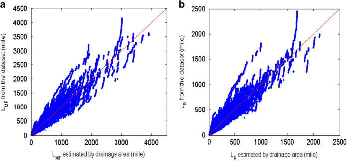
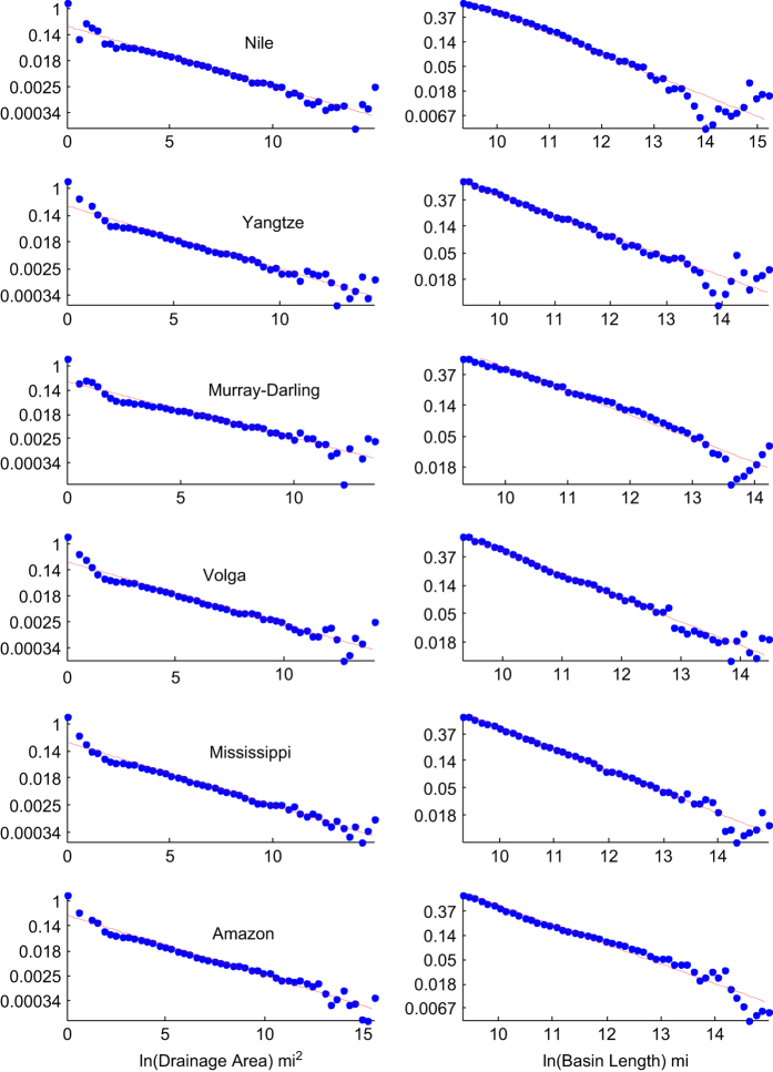
Scatter plots of equation (1) with setting L to L_MF and L_B are given in Fig. 3a,b. The Pearson correlation coefficient varies from 0.96 to 0.99 and the root mean squared error (RMSE) varies from 10.95 to 41.67 mi for L_MF and from 4.982 to 12.00 mi for L_B, respectively, as given in Table 2. The linearity of the pdf of equations (7) and (8) are tested in the following river basins, Nile, Yangtze, Mississippi, Amazon, Murray-Darling and Volga Rivers, as shown in Fig. 4. The goodness of fit of the distribution and the estimated β and γ are listed in Table 3. Except the slight deviation at both ends, the overall power law distribution is very well represented by the proposed dataset with obtaining Pearson correlation coefficients from 0.89–0.98, and the estimated β fallen between 0.4–0.5 (indicating that n is between 0.5–0.6). At this point, we have proved that the proposed data satisfy the Hack’s law.

Figure 3. Validation of the Hack’s law:

(a) basin area versus main flow length and (b) basin area versus basin length. The correlation value and RMSE of this fitting are given in Table 2.

Table 2. Fitting error and coefficients of the Hack’s law.

	AF	AS	AU	NA	CA	SA	EU	AF	AS	AU	NA	CA	SA	EU
	Pearson Correlation							RMSE (mi)
LMF	0.9828	0.9633	0.9754	0.9875	0.9912	0.9798	0.9760	25.60	41.67	15.97	22.11	10.95	31.79	21.23
LB	0.9765	0.9629	0.9680	0.9837	0.9846	0.9782	0.9668	9.695	12.00	6.415	7.520	4.982	10.39	7.840
	C							n
LMF	1.8102	1.4318	1.8672	1.9455	0.8945	2.8166	2.1845	0.5329	0.5715	0.5268	0.5326	0.6157	0.4944	0.5168
LB	2.0910	1.7300	1.9922	2.0133	0.9584	2.8204	2.3020	0.4808	0.5048	0.4825	0.4829	0.5696	0.4526	0.4641

Figure 4. Validation of the PDF of drainage area and basin length given by equations (7) and (8) in the left and right column respectively.

Each row contains the results from a river. From the top to the bottom, they are Nile River in Africa, Yangtze River in Asia, Murray–Darling River in Australia, Volga River in Europe, Mississippi River in North America, and Amazon River in South America.

Table 3. Slope and the goodness of-fit of equations (7) and (8).

	Nile	Yangtze	Murray-Darling	Mississippi	Amazon	Volga	Nile	Yangtze	Murray-Darling	Mississippi	Amazon	Volga
Pearson Correlation							Slope (β for p(B) and γ for p(M))
p(B)	0.9312	0.9346	0.8935	0.9590	0.9568	0.9210	0.4679	0.4667	0.4628	0.4621	0.4853	0.4798
p(M)	0.9196	0.9345	0.9485	0.9736	0.9594	0.9753	0.8566	0.7536	0.7671	0.7907	0.8080	0.8243

Additional information

How to cite this article: Shen, X. et al. A global distributed basin morphometric dataset. Sci. Data 4:160124 doi: 10.1038/sdata.2016.124 (2017).

Publisher’s note: Springer Nature remains neutral with regard to jurisdictional claims in published maps and institutional affiliations.

References

- Twidale C. River patterns and their meaning. Earth-Science Reviews 67, 159–218 (2004). [Google Scholar]
- Ibanez D. M., Riccomini C. & de Miranda F. P. Geomorphological evidence of recent tilting in the Central Amazonia Region. Geomorphology 214, 378–387 (2014). [Google Scholar]
- Seoane J. C. S. C. & de Barros Silva A. R. Gold—anomalous catchment basins: a GIS prioritization model considering drainage sinuosity. Journal of Geochemical Exploration 67, 335–344 (1999). [Google Scholar]
- Han Z., Wu L., Ran Y. & Ye Y. The concealed active tectonics and their characteristics as revealed by drainage density in the North China plain (NCP). Journal of Asian Earth Sciences 21, 989–998 (2003). [Google Scholar]
- Church M. & Ferguson R. Morphodynamics: Rivers beyond steady state. Water Resour. Res. 51, 1883–1897 (2015). [Google Scholar]
- Zhang S., Guo Y. & Wang Z. Correlation between flood frequency and geomorphologic complexity of rivers network–a case study of Hangzhou China. J. Hydrol. 527, 113–118 (2015). [Google Scholar]
- Pardo-Iguzquiza E., Durán-Valsero J. J. & Rodríguez-Galiano V. Morphometric analysis of three-dimensional networks of karst conduits. Geomorphology 132, 17–28 (2011). [Google Scholar]
- De Scally F., Owens I. & Louis J. Controls on fan depositional processes in the schist ranges of the Southern Alps, New Zealand, and implications for debris-flow hazard assessment. Geomorphology 122, 99–116 (2010). [Google Scholar]
- Di Lazzaro M., Zarlenga A. & Volpi E. Hydrological effects of within-catchment heterogeneity of drainage density. Advances in Water Resources 76, 157–167 (2015). [Google Scholar]
- Costa J. E. Hydraulics and basin morphometry of the largest flash floods in the conterminous United States. J. Hydrol. 93, 313–338 (1987). [Google Scholar]
- Glade T. Linking debris-flow hazard assessments with geomorphology. Geomorphology 66, 189–213 (2005). [Google Scholar]
- Raux J., Copard Y., Laignel B., Fournier M. & Masseï N. Classification of worldwide drainage basins through the multivariate analysis of variables controlling their hydrosedimentary response. Global and Planetary Change 76, 117–127 (2011). [Google Scholar]
- Lehner B., Verdin K. & Jarvis A. New global hydrography derived from spaceborne elevation data. Eos 89, 93–94 (2008). [Google Scholar]
- (ed NASA LP DAAC) (NASA EOSDIS Land Processes DAAC, USGS Earth Resources Observation and Science (EROS) Center, Sioux Falls, South Dakota https://lpdaac.usgs.gov (2015).
- Simley J. D. & Carswell Jr W. J. The National Map—Hydrography: U.S. Geological Survey Fact Sheet 4, 2009–3054 (2009). [Google Scholar]
- Wu H., Kimball J. S., Mantua N. & Stanford J. Automated upscaling of river networks for macroscale hydrological modeling. Water Resour. Res. 47, W03517 (2011). [Google Scholar]
- Altın T. B. The Flood Risk of the Yeşilırmak Basin (upper course), Turkey. Procedia-Social and Behavioral Sciences 120, 460–467 (2014). [Google Scholar]
- Rowberry M. D. A comparison of three terrain parameters that may be used to identify denudation surfaces within a GIS: A case study from Wales, United Kingdom. Computers & Geosciences 43, 147–158 (2012). [Google Scholar]
- Guth P. Drainage basin morphometry: a global snapshot from the shuttle radar topography mission. Hydrology and Earth System Sciences 15, 2091–2099 (2011). [Google Scholar]
- Hack J. Studies of longitudinal profiles in Maryland and Virginia, US Geol. Sum. Prof. Pap. B 294, 45–92 (1957). [Google Scholar]
- Shen X. et al. GDBC: A tool for generating global-scale distributed basin morphometry. Environmental Modelling & Software 83, 212–223 (2016). [Google Scholar]
- Lehner B., Verdin K. & Jarvis A. HydroSHEDS technical documentation, version 1.0. World Wildlife Fund US, Washington, DC 1–27 (2006). [Google Scholar]
- Mueller J. E. Re-evaluation of the relationship of master streams and drainage basins. Geological Society of America Bulletin 83, 3471–3474 (1972). [Google Scholar]
- Mesa O. J. & Gupta V. K. On the main channel length‐area relationship for channel networks. Water Resour. Res. 23, 2119–2122 (1987). [Google Scholar]
- Rigon R. et al. On Hack’s law. Water Resour. Res. 32, 3367–3374 (1996). [Google Scholar]
- Maritan A., Rinaldo A., Rigon R., Giacometti A. & Rodríguez-Iturbe I. Scaling laws for river networks. Physical review E—Statistical Physics, Plasmas, Fluids, and Related Interdisciplinary Topics 53, 1510–1515 (1996). [DOI] [PubMed] [Google Scholar]
- Rinaldo A., Rodriguez-Iturbe I. & Rigon R. Channel networks. Annual Review of Earth and Planetary Sciences 26, 289–327 (1998). [Google Scholar]
- Strahler A. N. Dynamic basis of geomorphology. Geological Society of America Bulletin 63, 923–938 (1952). [Google Scholar]
- Horton R. E. Erosional development of streams and their drainage basins; hydrophysical approach to quantitative morphology. Geological society of America bulletin 56, 275–370 (1945). [Google Scholar]
- Mueller J. E. An introduction to the hydraulic and topographic sinuosity indexes 1. Annals of the Association of American Geographers 58, 371–385 (1968). [Google Scholar]
- Gregory K. & Walling D. The variation of drainage density within a catchment. Hydrological Sciences Journal 13, 61–68 (1968). [Google Scholar]
- Schumm S. A. Evolution of drainage systems and slopes in badlands at Perth Amboy, New Jersey. Geological Society of America Bulletin 67, 597–646 (1956). [Google Scholar]
- Te Chow V. Advances in hydroscience Vol. 1 452 (Academic Press, 1964). [Google Scholar]
- Strahler A. N. in Handbook of applied hydrology, edCHOW VT ED.Mc Graw-Hill, 1964). [Google Scholar]
- Wolman M. G. & Miller J. P. Magnitude and frequency of forces in geomorphic processes. The Journal of Geology 68, 54–74 (1960). [Google Scholar]
- Horton R. E. Drainage‐basin characteristics. Eos, Transactions American Geophysical Union 13, 350–361 (1932). [Google Scholar]
- Miller O. & Summerson C. H. Slope-zone maps. Geographical Review 50, 194–202 (1960). [Google Scholar]
- Chorley R. J. Illustrating the laws of morphometry. Geological Magazine 94, 140–150 (1957). [Google Scholar]
- Gravelius H. Flusskunde (Berlin, Goschensche Verlagshandlung, 1914).
- Smart J. & Surkan A. The relation between mainstream length and area in drainage basins. Water Resour. Res. 3, 963–974 (1967). [Google Scholar]
- Melton M. A. An analysis of the relations among elements of climate, surface properties, and geomorphology (DTIC Document, 1957). [Google Scholar]
- Faniran A. The index of drainage intensity-A provisional new drainage factor. Australian Journal of Science 31, 328–330 (1968). [Google Scholar]
- Strahler A. in The Encyclopedia of Geomorphology (ed. Fairbridge R. W.) (Reinhold Book Corporation, 1968). [Google Scholar]
Associated Data
This section collects any data citations, data availability statements, or supplementary materials included in this article.
Data Citations
- Shen X. 2016. Figshare. http://dx.doi.org/10.6084/m9.figshare.c.3302111