Impact of analysing continuous outcomes using final values, change scores and analysis of covariance on the performance of meta‐analytic methods: a simulation study

Abstract

When meta‐analysing intervention effects calculated from continuous outcomes, meta‐analysts often encounter few trials, with potentially a small number of participants, and a variety of trial analytical methods. It is important to know how these factors affect the performance of inverse‐variance fixed and DerSimonian and Laird random effects meta‐analytical methods. We examined this performance using a simulation study.

Meta‐analysing estimates of intervention effect from final values, change scores, ANCOVA or a random mix of the three yielded unbiased estimates of pooled intervention effect. The impact of trial analytical method on the meta‐analytic performance measures was important when there was no or little heterogeneity, but was of little relevance as heterogeneity increased. On the basis of larger than nominal type I error rates and poor coverage, the inverse‐variance fixed effect method should not be used when there are few small trials.

When there are few small trials, random effects meta‐analysis is preferable to fixed effect meta‐analysis. Meta‐analytic estimates need to be cautiously interpreted; type I error rates will be larger than nominal, and confidence intervals will be too narrow. Use of trial analytical methods that are more efficient in these circumstances may have the unintended consequence of further exacerbating these issues. © 2015 The Authors. Research Synthesis Methods published by John Wiley & Sons, Ltd. © 2015 The Authors. Research Synthesis Methods published by John Wiley & Sons, Ltd.

1. Introduction

Systematic reviews are a valuable tool for informing decisions about health care. Meta‐analyses of randomised trials often form an important component of systematic reviews, from which conclusions about the effectiveness of healthcare interventions are drawn. Continuous outcomes are commonly evaluated in systematic reviews (Davey et al., 2011) and are of particular importance in, for example, psychological and psychiatric healthcare interventions musculoskeletal interventions and nutrition interventions. Complexity in combining the effects of interventions from continuous outcomes measured on the same scale arises from factors such as the variety of analytical methods used in the component trials, the size of the trials (which are typically smaller compared with trials of binary primary outcomes (Davey et al., 2011)) and the number of trials per meta‐analysis (which are generally few) (Davey et al., 2011).

In many parallel group randomised trials, the continuous outcome is measured at baseline, before the intervention has occurred, and at one (pretest–posttest) or multiple follow‐up periods (pretest–posttest–follow‐up). Many analytical approaches exist for analysing continuous data from pretest–posttest randomised trials, where the approaches can be considered in three categories defined by the method used to adjust for the baseline variable. The baseline variable can be ignored (no adjustment) or can be adjusted using either ‘crude’ or ‘covariate’ adjustment. Commonly employed analytical methods representing each of these categories respectively (and further described in Section 2) include a simple analysis of final values (SAFV), simple analysis of change scores (SACS) and analysis of covariance (ANCOVA). The qualifier ‘simple analysis’ is borrowed from Senn (2006) to indicate that these approaches do not involve covariate adjustment.

The statistical properties of SAFV, SACS and ANCOVA have been extensively reviewed (e.g. (Senn, 1989; Senn, 1993; Wei and Zhang, 2001)). ANCOVA has been recommended in preference to SAFV and SACS on the grounds that it will generally yield the most efficient analysis (Wei and Zhang, 2001; Van Breukelen, 2006; Senn, 2007a; Borm et al., 2007), with the comparative efficiency between SAFV and SACS dependent on the correlation between the baseline and follow‐up measurements. Moreover, for trialists concerned about observed baseline imbalance, ANCOVA yields unbiased estimates of intervention effect and maintains the nominal type I error rate, conditional on the observed baseline imbalance, which both SAFV and SACS do not (Senn, 1993; Wei and Zhang, 2001). At the meta‐analytic level, bias resulting from baseline imbalance is arguably of less relevance; across a series of properly conducted randomised trials, baseline imbalance will randomly vary about zero, resulting in overestimation of the intervention effect for some trials, but for an equal proportion of trials, underestimation of the intervention effect. However, it is of interest to examine the relative efficiency of meta‐analytic methods, which combine results generated from the three analytical methods, and further, how the properties of the meta‐analytic methods may be affected by violations in assumptions of the analytical methods at the trial level (e.g. heteroscedasticity in follow‐up variances and heterogeneity of slopes).

Inverse‐variance fixed and random effects meta‐analytic methods weight the intervention effects by the reciprocal of their variance. These meta‐analytic methods have wide appeal because of their extensive application (e.g. pooling different metrics of intervention effect, from different study designs and from more complex models). Across a set of randomised trials with continuous outcomes measured using the same scale (e.g. systolic blood pressure and Hamilton Depression Rating Scale), estimates of intervention effect from SAFV, SACS and ANCOVA can easily be combined using the inverse‐variance method. Under the fixed effect model, the variances of the effect estimates are assumed to be known, and inference is made assuming the pooled estimates of intervention effect are normally distributed (Normand, 1999). In practice, the variances are unknown and have to be estimated. For trials of at least a moderate size, the within‐trial variances can be adequately estimated; however, for small trials, this need not be so, and the resulting estimate of variance of the pooled effect may be compromised.

Further complexity arises in the case of random effects meta‐analysis, which additionally involves estimation of the between‐trial variance. The commonly used method of moments estimator, proposed by DerSimonian and Laird (1986), ignores uncertainty in the estimation of the between‐trial variance. Shortcomings of the DerSimonian and Laird random effects method have long been recognised (e.g. (Hardy and Thompson, 1996; Follmann and Proschan, 1999; Brockwell and Gordon, 2001; Hartung and Knapp, 2001; Ziegler et al., 2001; Sanchez‐Meca and Marin‐Martinez, 2008)), which has led to development of methods that attempt to allow for imprecision in the estimate of the between‐trial variance (e.g. marginal profile method (Hardy and Thompson, 1996)). These methods are often more complex to implement and may still be problematic when there are a small number of trials (Brockwell and Gordon, 2001; Borenstein et al., 2010).

There has been little research examining how inverse variance meta‐analytical methods perform for continuous outcomes, and how the choice of trial analytical method may affect this performance. Banerjee et al. (2008) examined through statistical simulation the impact of meta‐analysing SAFV and SACS, in different combinations, on bias, precision and statistical significance. This investigation did not consider ANCOVA and was limited to fixed effect meta‐analysis. Riley et al. (2013) illustrated through four case examples different methods for meta‐analysing data from pretest–posttest randomised trials (including ANCOVA, SAFV and SACS), considering scenarios with and without access to individual participant data and with and without baseline imbalance between intervention groups.

In this paper, we aim to extend and address gaps in previous research by using statistical simulation to examine how inverse‐variance fixed and random effects meta‐analytical methods perform for continuous outcomes across a wide range of scenarios. We focus on circumstances where the assumptions of the meta‐analysis methods may not be met and examine how the trial analytical method (SAFV, SACS and ANCOVA) may impact on the performance. We begin by describing the assumed distributions of data (on which the simulations are based) and the resulting implied models and provide a brief review of the trial analytical methods and meta‐analysis models in Section 2. In Section 3, we outline the simulation study methods. The results from the simulation study are presented in Section 4 and discussed in Section 5.

2. A review of the trial analytical methods and meta‐analysis models

We begin by describing notation, the assumed distributions of data and resulting implied models. Let Y represent the observed continuous outcome variable measured at follow‐up and X the baseline measure of this outcome variable. We assume that X and Y follow a bivariate normal distribution. More specifically, we assume that the measurements from the control group (ctrl) in a particular trial i, follow a bivariate normal distribution with the following parameters:

$$\left(\begin{array}{c}\hfill X_{ctr{l}_i}\hfill \\ \hfill Y_{ctr{l}_i}\hfill \end{array}\right)~BVN\left(\left(\begin{array}{c}\hfill 0\hfill \\ \hfill \alpha \hfill \end{array}\right),\left(\begin{array}{cc}\hfill 1\hfill & \hfill \rho \hfill \\ \hfill \rho \hfill & \hfill 1\hfill \end{array}\right)\right)\text{,}$$ (1)

where ρ is the correlation between the baseline and follow‐up measurements and α is the mean at follow‐up, representing change in the mean outcome over time. The variance of the measurements at both baseline ( ${\sigma }_{X_{\mathit{\text{ctrl}}}}^2$) and follow‐up ( ${\sigma }_{Y_{\mathit{\text{ctrl}}}}^2$) is assumed to be one. In the intervention group (int), we assume the measurements follow:

$$\left(\begin{array}{c}\hfill X_{\mathit{\text{in}}{t}_i}\hfill \\ \hfill Y_{\mathit{\text{in}}{t}_i}\hfill \end{array}\right)~BVN\left(\left(\begin{array}{c}\hfill 0\hfill \\ \hfill \theta +\alpha +u_i\hfill \end{array}\right),\left(\begin{array}{cc}\hfill 1\hfill & \hfill \rho {\sigma }_{Y_{int}}\hfill \\ \hfill \rho {\sigma }_{Y_{int}}\hfill & \hfill {\sigma }_{Y_{int}}^2\hfill \end{array}\right)\right)\text{,}$$ (2)

where α is as defined in Equation 1, θ represents the mean intervention effect across all trials and u _i represents a random effect, which allows for the intervention effect to vary across trials, and is distributed as follows:

$$u_i~N\left(0,{\tau }^2\right)\text{,}$$ (3)

with τ ² representing the between‐trial (heterogeneity) variance. The parameter θ is our target parameter for inference in this paper. The correlation (ρ) is assumed to be the same in the intervention and control groups. The variance at baseline ( ${\sigma }_{X_{int}}^2)$ is assumed to be 1, and at follow‐up ${\sigma }_{Y_{int}}^2$. The bivariate normal model implies the expected mean of Y _a conditional on X _a is (Larsen and Marx, 1986):

$$E\left(Y_a|X_a,u_i,T\right)=\alpha +\left(\theta +u\right)T+\rho {\sigma }_{Y_a}{X}_a\text{,}$$

where a represents either the intervention or control group, T is an indicator variable representing the intervention group (i.e. T = I(a = int)) and u represents the expected value of the random effects. The product $\rho {\sigma }_{Y_a}={\beta }_a$ describes the slope of the linear relationship between the baseline and follow‐up measurements, which under the assumed distributions of data may differ by intervention group if the variance of the follow‐up measurements differs (i.e. if ${\sigma }_{Y_{int}}^2\ne {\sigma }_{Y_{\mathit{\text{ctrl}}}}^2=1$).

2.1. Methods for analysing randomised trials with continuous outcomes

2.1.1. Simple analysis of final values

An estimate of the intervention effect θ can be calculated simply as the difference in means at follow‐up between groups:

$${\widehat{\theta }}_{SAF{V}_i}={\overline{Y}}_{int}-{\overline{Y}}_{\mathit{\text{ctrl}}}$$

with the variance calculated as

$$\widehat{Var}\left({{\widehat{\theta }}_{\mathit{\text{SAFV}}}}_{\mathit{i}}\right)=S{D}_{Y_P}^2\left(\frac{1}{n_{int}}+\frac{1}{n_{\mathit{\text{ctrl}}}}\right)\text{,}$$

where n _int and n _ctrl represent the sample sizes per intervention group and $S{D}_{Y_P}^2$ is an estimate of the pooled variance of the measurements at follow‐up and is calculated as

$$S{D}_{Y_P}^2=\frac{\left(n_{int}-1\right)S{D}_{Y_{int}}^2+\left(n_{\mathit{\text{ctrl}}}-1\right)S{D}_{Y_{\mathit{\text{ctrl}}}}^2}{\left(n_{int}+n_{\mathit{\text{ctrl}}}-2\right)}\text{,}$$

with $S{D}_{Y_{int}}^2$ and $S{D}_{Y_{\mathit{\text{ctrl}}}}^2$ being the sample estimates of the variance of measurements at follow‐up in the intervention and control groups, respectively, where the underlying variances are assumed equal across intervention groups. This estimate of intervention effect and its variance can be obtained by least squares from a regression model with final values as the outcome and the intervention group included as a binary explanatory variable. This model ignores the relationship between baseline and follow‐up measurements, and it assumes equal error variances.

2.1.2. Simple analysis of change scores

An alternative estimate of the intervention effect θ can be obtained by computing a change score for each participant (i.e. CS = Y − X) and then calculating the difference in mean change between groups:

$${{\widehat{\theta }}_{\mathit{\text{SACS}}}}_i=\left({\overline{Y}}_{int}-{\overline{X}}_{int}\right)-\left({\overline{Y}}_{\mathit{\text{ctrl}}}-{\overline{X}}_{\mathit{\text{ctrl}}}\right)=\left({\overline{Y}}_{int}-{\overline{Y}}_{\mathit{\text{ctrl}}}\right)-\left({\overline{X}}_{int}-{\overline{X}}_{\mathit{\text{ctrl}}}\right)$$

with the variance calculated as

$$\widehat{Var}\left({{\widehat{\theta }}_{\mathit{\text{SACS}}}}_{\mathit{i}}\right)=S{D}_{C{S}_P}^2\left(\frac{1}{n_{int}}+\frac{1}{n_{\mathit{\text{ctrl}}}}\right)\text{,}$$

where $S{D}_{C{S}_P}^2$ is an estimate of the pooled variance of change scores and is calculated as

$$S{D}_{C{S}_P}^2=\frac{\left(n_{int}-1\right)S{D}_{{CS}_{int}}^2+\left(n_{\mathit{\text{ctrl}}}-1\right)S{D}_{{CS}_{ctrl}}^2}{\left(n_{int}+n_{\mathit{\text{ctrl}}}-2\right)}$$

with $S{D}_{C{S}_{\mathit{\text{int}}}}^2$ and $S{D}_{C{S}_{\mathit{\text{ctrl}}}}^2$ being the sample estimates of the variance of change scores in the intervention and control groups, respectively, where the underlying variances are assumed equal across intervention groups. Sample estimates of the variance of change scores can also be calculated from the variances of measurements at baseline and follow‐up, and the correlation between the baseline and follow‐up measurements using

$$S{D}_{C{S}_a}^2=S{D}_{Y_a}^2+S{D}_{X_a}^2-2r_{a}S{D}_{Y_a}S{D}_{X_a}\text{,}$$

where a represents either the intervention or control group and r _a is the estimated correlation between the baseline and follow‐up measurements.

This estimate of intervention effect and its variance can be obtained by least squares using a regression model with change scores as the outcome, and the intervention group can be included as a binary explanatory variable. This model assumes that the slope between the baseline and follow‐up measurements is one in each group, implying that for every one‐unit increase in the baseline measure, a one‐unit increase would be expected in the follow‐up value (Bonate, 2000; Ganju, 2004). This model provides a ‘crude’ adjustment for the baseline measure in the sense that the implied correlation between the baseline and follow‐up measurements is one, which in practice, is unlikely to occur. The model assumes equal error variances.

2.1.3. Analysis of covariance

Covariate adjustment provides an alternative method to adjust for baseline imbalance. This adjustment can be achieved through fitting a regression model with final values (or change scores) as the outcome, and the intervention group included as a binary explanatory variable along with the baseline measure of the outcome. This specification of the model assumes equal slopes between the baseline and follow‐up measurements in each group and equal error variances. This modelling approach is commonly known as ANCOVA. The estimate of intervention effect is calculated as follows:

$${{\widehat{\theta }}_{\mathit{\text{ANCOVA}}}}_i=\left({\overline{Y}}_{int}-{\overline{Y}}_{\mathit{\text{ctrl}}}\right)-\widehat{\beta }\left({\overline{X}}_{int}-{\overline{X}}_{\mathit{\text{ctrl}}}\right)\text{,}$$

where $\hat{\beta }$ is the estimated slope from the regression model. Formula for the estimated variance of the ANCOVA estimate is available in the work of Armitage et al. (2002).

2.1.4. Comparison between the three methods

The three analytical methods can be easily compared using the simplifying assumptions that the variances of the baseline and follow‐up measurements are known and are equal (i.e. ${\sigma }_{Y_a}^2={\sigma }_{X_a}^2={\sigma }^2$), the correlation between baseline and follow‐up measurements are known and equal across groups and n _int = n _ctrl = n. We re‐express the ANCOVA estimator as a weighted average of the SAFV and SACS estimators (Senn, 1993), such that

$${{\widehat{\theta }}_{\mathit{\text{ANCOVA}}}}_i=\left(1-\rho \right){{\widehat{\theta }}_{\mathit{\text{SAFV}}}}_{\mathit{i}}+\rho {{\widehat{\theta }}_{\mathit{\text{SACS}}}}_{\mathit{i}}\text{.}$$

Under the simplifying assumption of equal variances, the estimate of intervention effect from an ANCOVA will lie between the SACS and SAFV estimates. When the correlation is close to zero, the ANCOVA estimate will be located towards the SAFV estimate; when the correlation is close to one, the ANCOVA estimate will be located towards the SACS estimate.

Under the noted simplifying assumptions, the variances of the trial analytical methods reduce to (Senn, 2007a)

$$Var\left({{\widehat{\theta }}_{\mathit{\text{SAFV}}}}_{\mathit{i}}\right)=\frac{2{\sigma }^2}{n}$$

$$Var\left({{\widehat{\theta }}_{\mathit{\text{SACS}}}}_{\mathit{i}}\right)=\frac{2{\sigma }^2}{n}\left(2\left(1-\rho \right)\right)$$

$$Var\left({{\widehat{\theta }}_{\mathit{\text{ANCOVA}}}}_{\mathit{i}}\right)=\frac{2{\sigma }^2}{n}\left(1-{\rho }^2\right)\text{.}$$

When the correlation is known, the ANCOVA estimate will have a smaller variance than SAFV or SACS because (1 − ρ ²) ≤ 2(1 − ρ) and (1 − ρ ²) ≤ 1, respectively. For correlations < 0.5, the SAFV estimate will have a smaller variance than the SACS, with this relationship reversed for correlations > 0.5.

2.2. Meta‐analysis models

The estimates of intervention effect obtained from either a SAFV, SACS or ANCOVA can be combined across the trials assuming either a fixed or random effects model. The fixed effect model assumes that there is one true intervention effect (θ) and that each trial yields an estimate $\left({\hat{\theta }}_{\mathit{i}}\right)$ of this true effect. This model may more descriptively be described as the common‐effect model (Borenstein et al., 2010). The model can be specified by

$${\widehat{\theta }}_i=\theta +{ϵ}_i$$

$${ϵ}_i~N\left(0,Var\left({\widehat{\theta }}_i\right)\right)\text{,}$$

where the effect estimate variance $\left(Var\left({\widehat{\theta }}_i\right)\right)$ is assumed known. Under this assumption, the maximum likelihood estimator of θ is a simple weighted average of the ${\widehat{\theta }}_{i}s$, with the optimal weights (W _i) given by the reciprocal of $Var\left({\widehat{\theta }}_i\right)$ (Normand, 1999). The inverse‐variance estimator of θ is given by

$$\widehat{\theta }=\frac{{\displaystyle \sum }{W}_i{\widehat{\theta }}_i}{{\displaystyle \sum }{W}_i}\text{,}$$

and the variance of this estimator is

$$Var\left(\widehat{\theta }\right)=\frac{1}{{\displaystyle \sum }{W}_i}\text{.}$$

The information contributed by any trial is reflected in the proportion of the weight that the trial contributes to the total sum of the weights.

The random effects model is more general compared with the fixed effect model, allowing for the true intervention effects to vary. The model can be specified by

$${\widehat{\theta }}_i=\theta +u_i+{ϵ}_i\text{,}$$

$$u_i~N\left(0,{\tau }^2\right)\text{,}$$

$${ϵ}_i~N\left(0,Var\left({\widehat{\theta }}_i\right)\right)\text{,}$$

where θ is the average intervention effect and u _i is a random effect that allows a separate intervention effect for each trial (θ + u _i). The trial intervention effects are assumed to be normally distributed about the average intervention effect with between‐trial variance τ ². ϵ _i represents the error in estimating a trial's true effect from a sample of participants. The random effects, u _i and ϵ _i, are assumed to be independent. Under the assumption that $Var\left({\widehat{\theta }}_i\right)$ and τ ² are known, the maximum likelihood estimate of θ is a weighted average of the ${\widehat{\theta }}_{i}s$, with the trial weights equal to the inverse of $Var\left({\widehat{\theta }}_i\right)+{\tau }^2$ (Normand, 1999). Different estimators of τ ² are available; however, the method of moments estimator proposed by DerSimonian and Laird (1986) is commonly used.

3. Simulation methods

In brief, the simulation study consisted of generating small randomised trials, analysing the trials using a range of analytical methods and meta‐analysing the estimated intervention effects using both fixed and random effects meta‐analysis. The number of randomised trials per meta‐analysis was randomly varied (from a uniform distribution of between three and eight trials per meta‐analysis). Design parameter values were combined using a fully factorial approach, with 60 000 replicate meta‐analyses generated per combination. Various criteria evaluating the performance of the meta‐analytic methods were calculated. An overview of the steps in the simulation study is presented in Figure 1.

Figure 1.

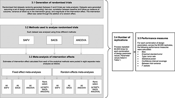
An overview of the steps in the simulation study. Titles in the boxes refer to section headings in the publication. SAFV, simple analysis of final values; ANCOVA, analysis of covariance; SACS, simple analysis of change scores

3.1. Generation of randomised trials

Randomised trials were generated by randomly sampling data from the bivariate normal distributions specified in Equations 1 and 2 (Section 2). Across simulation scenarios, the correlation between baseline and follow‐up measurements, ρ, was varied between 0 and 0.95 (Table 1) for both the control and intervention groups. A wide range of correlations was investigated because they are plausible in different applications (Frison and Pocock, 1992; Hewitt et al., 2010; Balk et al., 2012; Bell and McKenzie, 2013). For a particular simulation scenario, the trial datasets were constructed assuming a constant correlation.

Table 1.

Parameter values used in the simulation study.

Parameter	Values
Randomised trial
Analytical method	SAFV, SACS and ANCOVA
Correlation between baseline and follow‐up measurement of outcome (ρ)	0, 0.05, 0.25, 0.5, 0.75 and 0.95
Follow‐up intervention group variance ( ${\sigma }_{Y_{int}}^2$)	12 and 1.32
Intervention effect (θ)	0, 0.2, 0.5 and 0.8
Random effect (u i) allowing for between‐trial heterogeneity	u i ~ N(0, τ 2) where τ 2 = 0, 0.32, 0.62, 0.92
Change in the mean between baseline and follow‐up in each group (α)	0.1
Randomised trial size	N(20, 9)
Meta‐analyses
Number of trials per meta‐analysis	U(3, 8)
Combination of analytical methods used to analyse trials within a meta‐analysis	all SAFV, all SACS, all ANCOVA and random selection

SAFV, simple analysis of final values; ANCOVA, analysis of covariance; SACS, simple analysis of change scores.

The intervention effect, θ, was modelled as a shift in location of 0, 0.2, 0.5 and 0.8. These latter three shifts in location are Cohen's (Cohen, 1988) ‘small’, ‘moderate’ and ‘large’ effect sizes when the variance is one. The intervention effect was varied through the addition of the parameter u _i to allow for between‐trial heterogeneity, which may occur as a result of clinical or methodological diversity, or both. The random effect, u _i, was distributed N(0, τ ²), where τ ² was 0, 0.3², 0.6²or 0.9² representing no, low, moderate and high between‐trial heterogeneity, respectively. Assuming five trials per meta‐analysis, with 10 participants per group within each trial, equal variances of measurements at follow‐up of 1, and SAFV estimates, these heterogeneity parameters result in expected 95% prediction limits (and I ² values) of ±0.39 (0%), ±0.75 (61%), ±1.35 (76%) and ±1.97 (80%), respectively.

In the intervention group, the variance of the follow‐up measurements, ${\sigma }_{Y_{int}}^2$, was either 1 or 1.3². The latter value was included to investigate the effect of heteroscedasticity in follow‐up variances. Heteroscedasticity may occur when the intervention modifies the variation in the outcome, as may occur when the magnitude of intervention effect varies across participants.

The total size of each randomised trial was randomly sampled from a normal distribution with mean 20 and standard deviation of 3. A lower limit of a total of six participants was set, and randomised trials with fewer than this were discarded. The sample size was evenly distributed between the intervention and control groups. In instances where the total sample size was odd, the additional participant was randomly assigned with equal probability to either the intervention or control group.

3.2. Methods used to analyse randomised trials

The methods used to analyse the trial datasets were a SAFV, SACS and ANCOVA. These analyses were carried out using least squares regression using the models specified as described in Section 2.1.

3.3. Meta‐analysis of intervention effects

Estimates of intervention effect calculated from the analytical methods in each meta‐analysis were pooled using four combinations: (i) all SAFV, (ii) all SACS, (iii) all ANCOVA and (iv) a random selection of the three methods (each with equal probability of selection). Inverse‐variance weighting, using both fixed and random effects models, was used to combine the estimates. The method of moments estimator proposed by DerSimonian and Laird (1986) was used to estimate the between‐trial variance (τ ²) for use in the random effects analyses. Confidence intervals for the meta‐analytic effect were constructed using the Wald‐type method. The meta‐analytical methods were implemented using the ado package meta (Sharp and Sterne, 1997; Sharp and Sterne, 1998a; Sharp and Sterne, 1998b) in the statistical package stata (StataCorp, Texas, USA, 2007).

3.4. Number of replications

For each combination of design parameter values, 60 000 replicate meta‐analyses were created. For the performance measures type I error, power and coverage, this resulted in 95% confidence intervals of width less than 1% across all rates. This number of replicates allowed us to examine the effect of the number of trials per meta‐analysis on the performance measures with adequate power, providing at least 90% power to detect a difference in performance rates of 2.5% between two fixed values of the number of trials per meta‐analysis (e.g. meta‐analyses with three versus eight trials).

3.5. Performance measures

For each combination of design parameters, the results of the 60 000 meta‐analyses were assessed using the following performance measures: bias (the difference between the mean observed pooled intervention effect and the underlying intervention effect), empirical standard error (the standard deviation of observed pooled intervention effects across the simulations), type I error rate (the percentage of simulations for which the observed pooled intervention effect was significantly different from zero at the 5% level when the underlying intervention effect was zero), statistical power (the percentage of simulations for which the observed pooled intervention effect was significantly different from zero at the 5% level when the underlying intervention effect was greater than zero) and confidence interval coverage (the percentage of simulations for which the observed 95% confidence interval for the pooled intervention effect included the underlying intervention effect). In addition, two heterogeneity measures (between‐trial variance (τ ²) and a measure of the degree of inconsistency in intervention effects (I ²) (Higgins and Thompson, 2002)) were summarised.

3.6. Simulation procedures

Simulations were carried out using the statistical package stata (StataCorp, 2007). For each simulation scenario, a different starting seed was specified. A ‘moderately independent’ simulation design was used, where for each simulation scenario, the performance of fixed and random effects meta‐analysis was assessed on the same set of independently generated trial datasets (Figure 1) (Burton et al., 2006).

4. Results

4.1. Bias

For both fixed and random effects meta‐analysis, pooling estimates of intervention effect from randomised trials analysed by all SAFV, all SACS, all ANCOVA or a random selection resulted in unbiased estimates of pooled intervention effect across all simulation scenarios (maximum absolute bias was 0.004).

4.2. Precision

The precision (empirical standard errors) of the meta‐analytic estimators in these simulations are reflective of only sampling variability (which is a function of within‐trial and between‐trial variabilities), because there was no systematic bias. Across all simulation scenarios, precision was not modified by the underlying intervention effect. In scenarios with no between‐trial heterogeneity, precision of the fixed effect estimator was dependent on both the analytical methods employed in the trials and the correlation between the baseline and follow‐up measurements (Figure 2). The observed patterns were reflective of the relative efficiencies of the trial analytical methods. Combining all ANCOVA estimates resulted in either equivalent or increased precision compared with combining all SAFV, all SACS or a random selection. For correlations less than 0.5, combining all SAFV estimates resulted in increased precision compared with all SACS; this was reversed for correlations greater than 0.5. For any particular meta‐analysis, the estimate of the intervention effect could be substantially different from the underlying intervention effect; the use of ANCOVA being somewhat redeeming.

Figure 2.

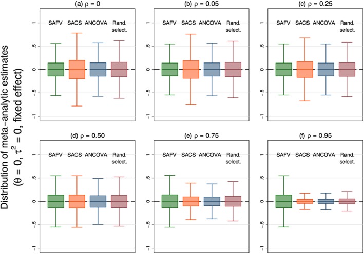
Box plots representing the distribution of meta‐analytic estimates calculated from four combinations of analytical methods (all SAFV, all SACS, all ANCOVA and Rand. select.) using a fixed effect model. Box plots represent simulation scenarios with θ = 0, ${\sigma }_{Y_{int}}^2=1$ and τ ² = 0. Separate plots represent different correlations. Note that outliers are not plotted. SAFV, simple analysis of final values; ANCOVA, analysis of covariance; SACS, simple analysis of change scores; Rand. select., random selection

The precision of the random effects estimator was less influenced by either the trial analytical method or correlation when there was between‐trial heterogeneity, particularly in simulation scenarios with high heterogeneity (Figure S1 in the Supporting Information).

4.3. Type I error rate

Type I error rates were always larger than nominal for fixed effect meta‐analysis (Figure 3). When there was no between‐trial heterogeneity, the type I error rate was invariant to the trial analytical method and correlation, with a mean rate of 7.9% over all analytical methods and correlations. Increasing between‐trial heterogeneity was associated with greater inflation of the type I error rate (ranging from 31% to 78% over all combinations of trial analytical methods and correlations when there was high heterogeneity). In the presence of heterogeneity, the fixed effect model is a misspecified model, and its performance is expected to be poor. Despite this, the fixed effect model is commonly applied in the presence of heterogeneity (Riley et al., 2011).

Figure 3.

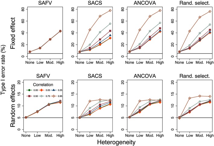
Plots of type I error rate (%) versus heterogeneity for the fixed and random effects meta‐analytical estimators calculated from four combinations of analytical methods (all SAFV, all SACS, all ANCOVA and Rand. select.). Plots represent simulation scenarios with θ = 0 and ${\sigma }_{Y_{int}}^2=1$. The horizontal line represents the nominal 5% type I error rate. Vertical scales differ for the fixed effect (top row) and random effects (bottom row) plots. SAFV, simple analysis of final values; ANCOVA, analysis of covariance; SACS, simple analysis of change scores; Rand. select., random selection

Type I error rates of the random effects meta‐analysis method were invariant to the trial analytical method and correlation when there was no heterogeneity (Figure 3) and were close to the nominal rate of 5% (ranging from 4.8% to 5.3% over all combinations of trial analytical methods and correlations). Increasing heterogeneity resulted in inflated (larger than nominal) type I error rates for all combinations of trial analytical methods (Figure 3). The degree of inflation was modified by correlation for combinations that included SACS and ANCOVA estimates. When there was high heterogeneity, type I error rates ranged from 10.7% to 14.0%, over all combinations of trial analytical methods and correlations.

4.4. Statistical power

The percentage of random effects meta‐analytic estimates that were significantly different from zero at the 5% level of significance for varying intervention effects is presented in Figure 4. In simulation scenarios with no heterogeneity, power resulting from both fixed and random effects methods was similar (results from the fixed effect method not shown), with differences between the methods occurring primarily as a result of the larger than nominal type I error rates observed from the fixed effect method. Predictably, power increased with larger intervention effects. However, the particular values of power need to be interpreted cautiously in the presence of larger than nominal type I error rates, as occurred when there was between‐trial heterogeneity (Figure 3). Power was dependent on the combination of analytical method and correlation for low‐to‐moderate heterogeneity, with meta‐analysis of all ANCOVA estimates always yielding equivalent or better power, but was less influenced by these factors for high levels of heterogeneity. Power decreased with increasing heterogeneity, particularly in simulation scenarios with moderate and large underlying intervention effects.

Figure 4.

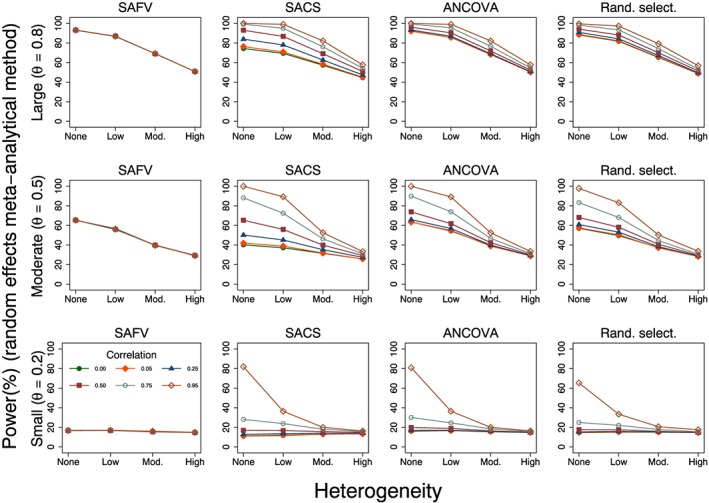
Plots of power (%) versus heterogeneity for the random effects meta‐analytic estimator calculated from four combinations of analytical methods (all SAFV, all SACS, all ANCOVA and Rand. select.) with ${\sigma }_{Y_{int}}^2=1$. Rows represent small, moderate and large underlying intervention effects. SAFV, simple analysis of final values; ANCOVA, analysis of covariance; SACS, simple analysis of change scores; Rand. select., random selection

4.5. Confidence interval coverage

The simulation results for coverage reflected those of type I error rate because no bias was observed in the meta‐analytic estimates of intervention effect. Coverage was always less than the nominal 95% level for fixed effect meta‐analysis and was invariant to the trial analytical method and correlation when there was no between‐trial heterogeneity (Figure 5). Furthermore, coverage was not affected by the magnitude of intervention effect; across these simulation scenarios, mean coverage was 92.0%.

Figure 5.

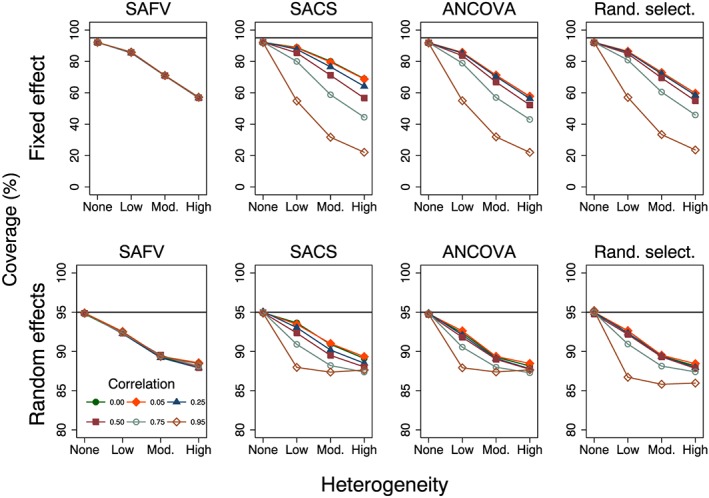
Plots of per cent coverage of 95% confidence intervals versus heterogeneity for the fixed and random effects meta‐analytical estimators calculated from four combinations of analytical methods (all SAFV, all SACS, all ANCOVA and Rand. select.). Plots represent simulation scenarios with θ = 0 and ${\sigma }_{Y_{int}}^2=1$. The horizontal line represents the nominal 95% coverage level. Vertical scales differ for the fixed effect (top row) and random effects (bottom row) plots. SAFV, simple analysis of final values; ANCOVA, analysis of covariance; SACS, simple analysis of change scores; Rand. select., random selection

For equivalent simulation scenarios, coverage levels resulting from random effects models were close to the nominal 95% level, with coverage ranging from 94.7% to 95.2% (Figure 5). Increasing heterogeneity resulted in increasingly anticonservative coverage levels for all analytical methods. For low and moderate heterogeneity, the coverage levels were associated with correlation for SACS and ANCOVA. However, for a particular level of heterogeneity, unless the correlations were extreme, the range of coverage levels for these two analytical methods did not differ to any important degree (Figure 5). When there was high heterogeneity, all combinations of analytical method and correlation resulted in similar coverage levels, ranging from 85.9% to 89.3%.

4.6. Heterogeneity measures

The mean estimates of DerSimonian and Laird's method of moments estimator of between‐trial variance $\left({\overline{\hat{\mathit{\tau }}}}^2\right)$ were invariant to the magnitude of treatment effect. The distributions of estimated between‐trial variance were positively skewed, with the particular shape of the distribution dependent on the combination of trial analytical method, correlation and the magnitude of the underlying heterogeneity parameter (τ ²) (Figure 6). In simulation scenarios with no underlying heterogeneity, τ ² was typically overestimated, while in the presence of heterogeneity, τ ² was underestimated in the majority of meta‐analyses.

Figure 6.

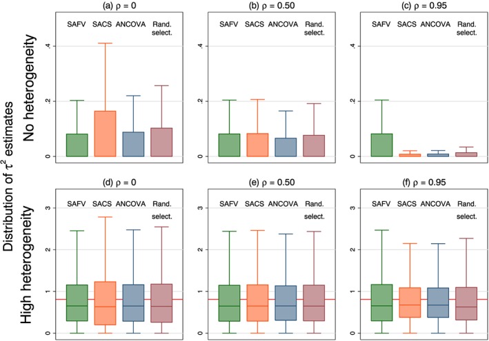
Box plots representing the distribution of τ ² estimates calculated from four combinations of analytical methods (all SAFV, all SACS, all ANCOVA and Rand. select.). Box plots represent select simulation scenarios with θ = 0 and ${\sigma }_{Y_{int}}^2=1$. The horizontal line in the bottom row represents underlying heterogeneity (τ ² = 0.9²). Vertical scales differ for the no (top row) and high (bottom row) heterogeneity plots. Note that outliers are not plotted. SAFV, simple analysis of final values; ANCOVA, analysis of covariance; SACS, simple analysis of change scores; Rand. select., random selection

The second measure of heterogeneity, the I ² statistic, was also invariant to the magnitude of intervention effect and appropriately reflected increasing underlying heterogeneity through increasing estimates of I ² (Figure 7). However, the I ² statistic was dependent on the combination of analytical methods and correlations and yielded variable estimates of I ² for the same underlying magnitude of heterogeneity when combining SACS, ANCOVA or a mix (e.g. mean I ² ranged from 67% (ρ = 0) to 95% (ρ = 0.95) when combining all ANCOVA estimates with τ ² = 0.9²). For a particular correlation, combining all ANCOVA yielded an equivalent or larger estimate of I ² compared with the largest I ² estimate from combining any of the other trial analytical methods. The distribution of I ² displayed extreme positive skew when there was no underlying heterogeneity, and in the presence of heterogeneity, the distribution of I ² was generally negatively skewed, with a cluster of estimates at zero.

Figure 7.

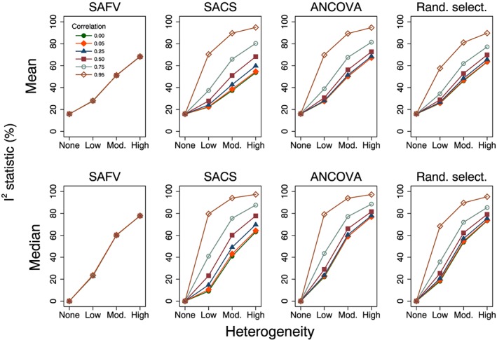
Plots of mean and median estimates of the I ² statistic (%) versus heterogeneity. Plots represent simulation scenarios with θ = 0 and ${\sigma }_{Y_{int}}^2=1$. SAFV, simple analysis of final values; ANCOVA, analysis of covariance; SACS, simple analysis of change scores; Rand. select., random selection

4.7. Impact of heteroscedasticity of follow‐up variances within trials on performance measures

Heteroscedasticity of follow‐up variances within randomised trials resulted in larger variances of intervention effects in the component trials, and in turn the meta‐analytic intervention effect. However, this increase in the variance of the meta‐analytic intervention effect did not result in any important differences across the performance measures (Figures S2–S8 in the Supporting Information).

4.8. Impact of the number of trials per meta‐analysis on performance measures

The number of randomised trials per meta‐analysis was allowed to randomly vary (between three and eight) in the simulation scenarios because we wished to examine the average performance of the meta‐analytic methods with a small number of randomised trials. We undertook some additional analyses to investigate if the performance measures bias and type I error rate were modified by the number of trials per meta‐analysis.

Examination of the simulation scenarios stratified by the number of trials per meta‐analysis revealed no relationship between this factor and bias. Both fixed and random effects meta‐analysis yielded unbiased estimates of pooled intervention effect for each simulation scenario stratified by the number of trials per meta‐analysis.

Type I error rates for both fixed and random effects meta‐analysis were not modified by the number of trials per meta‐analysis when there was no between‐trial heterogeneity. Examination of the type I error rates of the random effects method in the presence of heterogeneity revealed that the number of trials per meta‐analysis did modify type I error rates and, furthermore, that the degree of modification was dependent on the combination of trial analytical methods, correlation between the baseline and follow‐up measurements and magnitude of the underlying heterogeneity (Figure 8). However, the key determinants of differences in type I error rates were the number of trials per meta‐analysis and the underlying magnitude of heterogeneity. Type I error rates were larger when there were fewer trials per meta‐analysis. For example, combining all ANCOVA estimates with high underlying heterogeneity yielded type I error rates ranging from 9.1% (eight trials per meta‐analysis) to 17.9% (three trials per meta‐analysis), with an average type I error rate across all strata of 12.3% (Figure 8; plot in row 3, column 6).

Figure 8.

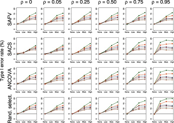
Plots of type I error rate (%) versus heterogeneity for the random effects meta‐analytical method. All plots represent simulation scenarios with θ = 0 and ${\sigma }_{Y_{int}}^2=1$. Separate plots depict each combination of analytical method (all SAFV, all SACS, all ANCOVA and Rand. select.), correlation and the number of trials per meta‐analysis. The number of trials per meta‐analysis is depicted by the following colours and symbols: 3 trials = solid green circle; 4 trials = solid orange diamond; 5 trials = solid navy triangle; 6 trials = solid maroon square; 7 trials = hollow teal circle; and 8 trials = hollow sienna diamond. The horizontal line represents the nominal 5% type I error rate. SAFV, simple analysis of final values; ANCOVA, analysis of covariance; SACS, simple analysis of change scores; Rand. select., random selection

5. Discussion

A frequently cited advantage of meta‐analysis is the ability to combine results from a series of small randomised trials to answer a question of effectiveness that could otherwise not be answered. In the case of randomised trials with primary continuous outcomes, the trials are generally smaller, and there are often only few trials included in a meta‐analysis. In these circumstances, the statistical properties of the meta‐analytical methods are most compromised. Further complexity arises from the different analytical methods available to adjust for the baseline measure of the outcome in the trials. The results of this simulation study have provided some insight into how the most commonly used standard inverse‐variance meta‐analytic methods perform in these circumstances.

The empirical standard errors of the meta‐analytic estimates for the examined simulation scenarios were generally large, particularly in the presence of moderate‐to‐high between‐trial heterogeneity, indicating that there was little precision in estimating the pooled intervention effect; some meta‐analytic estimates indicated substantial benefit, while others indicated substantial harm. When there was no heterogeneity, the trial analytical methods influenced precision and power of both the fixed and random effects meta‐analytic methods in an important way. In these circumstances, the performance measures of the meta‐analytic methods reflected the relative efficiencies of the trial analytical methods. This occurred because the weights of the fixed effect model are only a function of within‐trial variance, and in the case of random effects meta‐analysis, weights are primarily dependent on within‐trial variance when there is no underlying heterogeneity. Combining estimates from all ANCOVA yielded either equivalent or better precision compared with the analytical method (either all SAFV or all SACS) that had greatest precision for a particular correlation. Therefore, when the correlations differ across trials included in a meta‐analysis, the use of ANCOVA may be of particular benefit compared with combining either all SAFV or all SACS.

The importance of the trial analytical method on the precision and power of the random effects model became less relevant as between‐trial heterogeneity increased. Weights of the random effects model are a function of both within‐trial and between‐trial variances and, in the case of high heterogeneity, will primarily depend on between‐trial variance. Consequently, the choice of trial analytical method will become irrelevant.

Fixed effect meta‐analysis yielded larger than nominal type I error rates and confidence intervals that were too narrow. This observation was unsurprising because poor estimation of the within‐trial variances will compromise the estimate of variance of the pooled effect, with consequences for hypothesis testing and the calculation of confidence limits, which assume normality (Normand, 1999).

In contrast to fixed effect meta‐analysis, the random effects model (with the DerSimonian and Laird between‐trial variance estimator) provided a better solution; type I error rates and confidence interval coverage of the random effects model were closer to the nominal levels, and in the case of no heterogeneity, the random effects model yielded the correct type I error rate. This latter finding occurred because some datasets exhibited heterogeneity by chance, and in this circumstance, DerSimonian and Laird's method of moments estimator of τ ² yielded a positively biassed estimate. When this variance estimate was incorporated into the weights of the random effects model, the resulting standard errors of the meta‐analytic estimates were larger. This inflation of the standard error of the meta‐analytic estimate, for these simulation scenarios, fortuitously compensated for the imprecision in the estimates of within‐trial variance, resulting in the nominal type I error rate.

However, the random effects model did not provide a complete solution because it yielded larger than nominal type I error rates and confidence intervals that were too narrow in the presence of heterogeneity. This occurred primarily as a result of the underestimation of τ ² in the presence of heterogeneity. Estimation of τ ² was poorer when the underlying heterogeneity was larger, which resulted in a concomitant increase in the type I error rates; the DerSimonian and Laird method of moments estimator has been shown to be negatively biassed when τ ² is large (Sidik and Jonkman, 2007; Sidik and Jonkman, 2005). Furthermore, the degree of inflation was modified by the number of trials per meta‐analysis in the presence of moderate‐to‐high heterogeneity, with fewer trials resulting in larger type I error rates. Type I error rates in these circumstances were further exacerbated when all ANCOVA estimates were combined, a result of the distribution of ${\hat{\tau }}^2$ based on ANCOVA estimates having less variability compared with those distributions based on the other trial methods, and as such there being less compensation for poor estimation of the variance of the intervention effects.

In practice, for any particular meta‐analysis, when the between‐trial variance is estimated to be greater than zero, it will not be known if the observed variance is caused by real differences between‐trials or is as a result of poor estimation. Therefore, meta‐analysts will not be able to differentiate between situations where there truly is and is not heterogeneity, and thus, whether the nominal 5% type I error rate applies. This implies that even when the random effects model is employed, borderline findings of statistical significance need to be carefully interpreted; that is, not to falsely claim an intervention effect when the observed effect is more likely to be a result of chance. Particular care should be taken when there are only three or four trials.

The I ² statistic appropriately reflected increasing underlying heterogeneity through increasing estimates of I ². In the presence of heterogeneity, the statistic was influenced in an important way by the trial analytical method and the strength of correlation. The I ² statistic is not independent of the precisions of the estimates of intervention effect (Higgins and Thompson, 2002; Rucker et al., 2008). Therefore, I ² will differ for meta‐analyses where the underlying heterogeneity is the same, but the precisions of the estimates of intervention effect differ. In the case of SACS and ANCOVA, precision is a function of sample size and correlation; therefore, increasing correlation will result in larger values of I ². This finding provides additional justification for the recommendations of others that the decision of whether to synthesise the results, or choice of meta‐analytic model to use if the results are synthesised, should not be based on the I ² statistic (Ioannidis et al., 2008; Rucker et al., 2008; Riley et al., 2011).

Heteroscedasticity of follow‐up variances within randomised trials results in larger variances of intervention effects in the component trials, and in turn the meta‐analytic intervention effect. This increase in the variance of the pooled intervention effect did not result in any important differences across the performance measures. Importantly, ANCOVA provided equivalent or better performance compared with both SAFV and SACS when its assumptions were compromised (heterogeneity of slopes) and the trials were small.

Finally, we consider the generalisability of the results from our simulation study. In practice, meta‐analysts are likely to encounter a mix of SAFV, SACS and ANCOVA. The degree to which the results from these simulations are applicable will, in part, depend on the mechanisms underpinning the choice of trial analytical method. Our simulations are premised on this choice being made independent of the ensuing estimates of intervention effect (and their associated test statistics). For example, the results of our simulations would generalise to scenarios where, a priori, the choice of analytical method was based on the likely precision, or because the method was commonly used within a particular discipline. If the choice of analytical method is based on the ensuing estimates of intervention effect (e.g. selecting the most favourable of SACS or SAFV estimates), this will lead to bias in the meta‐analytic effect (McKenzie, 2011).

5.1. Strengths and limitations

This study provides an extension of previous research by examining through simulation the impact of ANCOVA, in addition to the more commonly employed SAFV and SACS (Banerjee et al., 2008). A particular strength of our simulation study is the wide range of simulation parameters and performance measures investigated for both the standard inverse‐variance fixed and random effects models. The chosen parameters were selected so that the simulation results would be applicable to commonly occurring scenarios.

A limitation of all simulation studies is that the results and ensuing interpretation depend on the selected parameters and methods chosen to construct the datasets. For example, the baseline and follow‐up measures in these simulations were generated assuming a bivariate normal distribution. Therefore, the performance of the trial analytical and meta‐analytical methods from these scenarios is likely to be more favourable than would be the case if the data were generated from non‐normal distributions. Choices over whether a simulation parameter is fixed or allowed to randomly vary in the construction of the datasets (e.g. fixing the underlying correlation and variances across trials within a meta‐analysis versus randomly selecting the correlations and variances from assumed distributions) may also impact on the simulation results.

5.2. Future research

The results of this study raise many questions that require further research. When the size of the trials are small, an alternative weighting system may be preferable, such as weighting by the number of participants (Senn, 2000; Senn, 2007b) or the effective sample size (Deeks et al., 2005). Further, investigation of alternative between‐trial variance estimators (e.g. Paule and Mandel (1982) and restricted maximum likelihood estimators (Raudenbush, 2009)) and methods to calculate confidence intervals for the pooled effect (e.g. Knapp and Hartung (1999)) are required. The use of Bayesian meta‐analysis methods that allow the incorporation of external estimates of between‐trial variance, where these estimates have been quantified from large datasets of meta‐analyses (e.g. Turner et al. (2012)), may be of particular value. Finally, while the focus of our research has been on the pooled effect and its confidence interval, examination of the performance of prediction intervals (Higgins et al., 2009) in the scenarios we have investigated would be valuable.

5.3. Conclusions

This simulation study has examined how standard inverse‐variance meta‐analytical methods perform when there are a small number of randomised trials including few participants, and how the type of analytical method employed at the trial level may impact on this performance. In general, type I error rates are likely to be larger than nominal, and the confidence intervals will be too narrow, particularly when there are only a small number of trials per meta‐analysis. Random effects meta‐analysis (with the DerSimonian and Laird between‐trial variance estimator) was shown to be preferable compared with fixed effect meta‐analysis. The trial analytical method was shown to affect the performance of the meta‐analytic methods when there was no or little heterogeneity. Results from meta‐analyses of few small trials should be cautiously interpreted.

Supporting information

 

Supporting info item

McKenzie, J. E. , Herbison, G. P. , and Deeks, J. J. (2016) Impact of analysing continuous outcomes using final values, change scores and analysis of covariance on the performance of meta‐analytic methods: a simulation study. Res. Syn. Meth., 7: 371–386. doi: 10.1002/jrsm.1196.

References

- Armitage P, Berry G, Matthews JNS 2002. Chapter 11: modelling continuous data In Statistical Methods in Medical Research. 4th edn. Oxford; Malden, MA: Blackwell Science Ltd. [Google Scholar]
- Balk EM, Earley A, Patel K, Trikalinos TA, Dahabreh IJ. 2012. Empirical assessment of within‐arm correlation imputation in trials of continuous outcomes. Methods Research Report. (Prepared by the Tufts Evidence‐based Practice Center under Contract No. 290‐2007‐10055‐I.). AHRQ Publication. Rockville, MD: Agency for Healthcare Research and Quality. [PubMed]
- Banerjee S, Wells GA, Chen L 2008. Caveats in the Meta‐analyses of Continuous Data: A Simulation Study. Ottawa: Canadian Agency for Drugs and Technologies in Health. [Google Scholar]
- Bell ML, Mckenzie JE 2013. Designing psycho‐oncology randomised trials and cluster randomised trials: variance components and intra‐cluster correlation of commonly used psychosocial measures. Psychooncology 22: 1738–1747. [DOI] [PubMed] [Google Scholar]
- Bonate PL 2000. Analysis of pretest–posttest designs In Chapter 1: Introduction. Boca Raton: Chapman & Hall/CRC. [Google Scholar]
- Borenstein M, Hedges LV, Higgins JPT, Rothstein HR 2010. A basic introduction to fixed‐effect and random‐effects models for meta‐analysis. Research Synthesis Methods 1: 97–111. [DOI] [PubMed] [Google Scholar]
- Borm GF, Fransen J, Lemmens WA 2007. A simple sample size formula for analysis of covariance in randomized clinical trials. Journal of Clinical Epidemiology 60: 1234–1238. [DOI] [PubMed] [Google Scholar]
- Brockwell SE, Gordon IR 2001. A comparison of statistical methods for meta‐analysis. Statistics in Medicine 20: 825–840. [DOI] [PubMed] [Google Scholar]
- Burton A, Altman DG, Royston P, Holder RL 2006. The design of simulation studies in medical statistics. Statistics in Medicine 25: 4279–4292. [DOI] [PubMed] [Google Scholar]
- Cohen J 1988. Statistical Power Analysis for the Behavioural Sciences. Hillsdale, New Jersey: Lawrence Erlbaum Associates, Inc. [Google Scholar]
- Davey J, Turner RM, Clarke MJ, Higgins JP 2011. Characteristics of meta‐analyses and their component studies in the Cochrane Database of Systematic Reviews: a cross‐sectional, descriptive analysis. BMC Medical Research Methodology 11: 160. [DOI] [PMC free article] [PubMed] [Google Scholar]
- Deeks JJ, Macaskill P, Irwig L 2005. The performance of tests of publication bias and other sample size effects in systematic reviews of diagnostic test accuracy was assessed. Journal of Clinical Epidemiology 58: 882–893. [DOI] [PubMed] [Google Scholar]
- Dersimonian R, Laird N 1986. Meta‐analysis in clinical trials. Controlled Clinical Trials 7: 177–188. [DOI] [PubMed] [Google Scholar]
- Follmann DA, Proschan MA 1999. Valid inference in random effects meta‐analysis. Biometrics 55: 732–737. [DOI] [PubMed] [Google Scholar]
- Frison L, Pocock SJ 1992. Repeated measures in clinical trials: analysis using mean summary statistics and its implications for design. Statistics in Medicine 11: 1685–1704. [DOI] [PubMed] [Google Scholar]
- Ganju J 2004. Reader reaction: some unexamined aspects of analysis of covariance in pretest–posttest studies. Biometrics 60: 829–833. [DOI] [PubMed] [Google Scholar]
- Hardy RJ, Thompson SG 1996. A likelihood approach to meta‐analysis with random effects. Statistics in Medicine 15: 619–629. [DOI] [PubMed] [Google Scholar]
- Hartung J 1999. An alternative method for meta‐analysis. Biometrical Journal 41: 901–916. [Google Scholar]
- Hartung J, Knapp G 2001. On tests of the overall treatment effect in meta‐analysis with normally distributed responses. Statistics in Medicine 20: 1771–1782. [DOI] [PubMed] [Google Scholar]
- Hewitt CE, Kumaravel B, Dumville JC, Torgerson DJ 2010. Assessing the impact of attrition in randomized controlled trials. Journal of Clinical Epidemiology 63: 1264–1270. [DOI] [PubMed] [Google Scholar]
- Higgins JP, Thompson SG 2002. Quantifying heterogeneity in a meta‐analysis. Statistics in Medicine 21: 1539–1558. [DOI] [PubMed] [Google Scholar]
- Higgins JPT, Thompson SG, Spiegelhalter DJ 2009. A re‐evaluation of random‐effects meta‐analysis. Journal of the Royal Statistical Society Series A‐Statistics in Society 172: 137–159. [DOI] [PMC free article] [PubMed] [Google Scholar]
- Ioannidis JP, Patsopoulos NA, Rothstein HR 2008. Reasons or excuses for avoiding meta‐analysis in forest plots. BMJ 336: 1413–1415. [DOI] [PMC free article] [PubMed] [Google Scholar]
- Larsen RJ, Marx M 1986. An Introduction to Mathematical Statistics and Its Applications. New Jersey: Prentice‐Hall. [Google Scholar]
- Mckenzie JE. 2011. Methodological issues in meta‐analysis of randomised controlled trials with continuous outcomes (PhD thesis). Doctor of Philosophy, Monash University.
- Normand SL 1999. Tutorial in biostatistics: meta‐analysis: formulating, evaluating, combining, and reporting. Statistics in Medicine 18: 321–359. [DOI] [PubMed] [Google Scholar]
- Paule RC, Mandel J 1982. Consensus values and weighting factors. Journal of Research of the National Bureau of Standards 87: 377–385. [DOI] [PMC free article] [PubMed] [Google Scholar]
- Raudenbush SW 2009. Analyzing effect sizes: random effects models In Cooper H, Hedges LV, Valentine JC. (eds.). The Handbook of Research Synthesis and Meta‐analysis. New York: Russell Sage Foundation. [Google Scholar]
- Riley RD, Gates S, Neilson J, Alfirevic Z 2011. Statistical methods can be improved within Cochrane pregnancy and childbirth reviews. Journal of Clinical Epidemiology 64: 608–618. [DOI] [PubMed] [Google Scholar]
- Riley RD, Kauser I, Bland M, Thijs L, Staessen JA, Wang J, Gueyffier F, Deeks JJ 2013. Meta‐analysis of randomised trials with a continuous outcome according to baseline imbalance and availability of individual participant data. Statistics in Medicine 32: 2747–2766. [DOI] [PubMed] [Google Scholar]
- Rucker G, Schwarzer G, Carpenter JR, Schumacher M 2008. Undue reliance on I2 in assessing heterogeneity may mislead. BMC Medical Research Methodology 8: 79. [DOI] [PMC free article] [PubMed] [Google Scholar]
- Sanchez‐Meca J, Marin‐Martinez F 2008. Confidence intervals for the overall effect size in random‐effects meta‐analysis. Psychological Methods 13: 31–48. [DOI] [PubMed] [Google Scholar]
- Senn S 2000. Letter to the editor. Controlled Clinical Trials 21: 589–592. [DOI] [PubMed] [Google Scholar]
- Senn S 2006. Change from baseline and analysis of covariance revisited. Statistics in Medicine 25: 4334–4344. [DOI] [PubMed] [Google Scholar]
- Senn S 2007a. Chapter 7: baselines and covariate information In Statistical Issues in Drug Development. 2nd edn. Chichester: John Wiley & Sons Ltd. [Google Scholar]
- Senn S 2007b. Chapter 16: meta‐analysis In Statistical Issues in Drug Development. 2nd edn. Chichester: John Wiley & Sons Ltd. [Google Scholar]
- Senn SJ 1989. Covariate imbalance and random allocation in clinical trials. Statistics in Medicine 8: 467–475. [DOI] [PubMed] [Google Scholar]
- Senn SJ 1993. Letter to the editor: baseline distribution and conditional size. Journal of Biopharmaceutical Statistics 3: 265–270. [DOI] [PubMed] [Google Scholar]
- Sharp S, Sterne J 1997. sbe16: meta‐analysis. Stata Technical Bulletin 38: 9–14. [Google Scholar]
- Sharp S, Sterne J 1998a. sbe16.1: new syntax and output for the meta‐analysis command. Stata Technical Bulletin 42: 6–8. [Google Scholar]
- Sharp S, Sterne J 1998b. sbe16.2: corrections to the meta‐analysis command. Stata Technical Bulletin 43: 15. [Google Scholar]
- Sidik K, Jonkman JN 2005. Simple heterogeneity variance estimation for meta‐analysis. Journal of the Royal Statistical Society: Series C: Applied Statistics 54: 367–384. [Google Scholar]
- Sidik K, Jonkman JN 2007. A comparison of heterogeneity variance estimators in combining results of studies. Statistics in Medicine 26: 1964–1981. [DOI] [PubMed] [Google Scholar]
- STATACORP 2007. Stata Statistical Software: Release 10. College Station, TX: StataCorp LP. [Google Scholar]
- Turner RM, Davey J, Clarke MJ, Thompson SG, Higgins JPT 2012. Predicting the extent of heterogeneity in meta‐analysis, using empirical data from the Cochrane Database of Systematic Reviews. International Journal of Epidemiology . [DOI] [PMC free article] [PubMed] [Google Scholar]
- Van Breukelen GJ 2006. ANCOVA versus change from baseline: more power in randomized studies, more bias in nonrandomized studies. Journal of Clinical Epidemiology 59: 920–925. [DOI] [PubMed] [Google Scholar]
- Wei L, Zhang J 2001. Analysis of data with imbalance in the baseline outcome variable for randomized clinical trials. Drug Information Journal 35: 1201–1214. [Google Scholar]
- Ziegler S, Koch A, Victor N 2001. Deficits and remedy of the standard random effects methods in meta‐analysis. Methods of Information in Medicine 40: 148–155. [PubMed] [Google Scholar]
Associated Data
This section collects any data citations, data availability statements, or supplementary materials included in this article.
Supplementary Materials