Gradient Pre-Emphasis to Counteract First-Order Concomitant Fields on Asymmetric MRI Gradient Systems

Abstract

PURPOSE

To develop a gradient pre-emphasis scheme that prospectively counteracts the effects of the first-order concomitant fields for any arbitrary gradient waveform played on asymmetric gradient systems, and to demonstrate the effectiveness of this approach using a real-time implementation on a compact gradient system.

METHODS

After reviewing the first-order concomitant fields that are present on asymmetric gradients, a generalized gradient pre-emphasis model assuming arbitrary gradient waveforms is developed to counteract their effects. A numerically straightforward, simple to implement approximate solution to this pre-emphasis problem is derived, which is compatible with the current hardware infrastructure used on conventional MRI scanners for eddy current compensation. The proposed method was implemented on the gradient driver sub-system, and its real-time use was tested using a series of phantom and in vivo data acquired from 2D Cartesian phase-difference, echo-planar imaging (EPI) and spiral acquisitions.

RESULTS

The phantom and in vivo results demonstrate that unless accounted for, first-order concomitant fields introduce considerable phase estimation error into the measured data and result in images exhibiting spatially dependent blurring/distortion. The resulting artifacts are effectively prevented using the proposed gradient pre-emphasis.

CONCLUSION

An efficient and effective gradient pre-emphasis framework is developed to counteract the effects of first-order concomitant fields of asymmetric gradient systems.

INTRODUCTION

As a consequence of Maxwell’s equations, the linear spatial encoding gradient fields used in conventional clinical magnetic resonance imaging (MRI) are always accompanied by additional undesired magnetic fields termed concomitant or Maxwell fields, which causes the actual magnetic field used for spatial encoding to deviate from the desired uniform gradient fields (1,2). These concomitant fields are present whenever gradients are active (i.e., throughout spatial encoding and data acquisition), and result in the accumulation of undesirable spatiotemporally-varying phase components within the measured data set. When this accumulated phase is not accounted for during MR image reconstruction, it can cause image artifacts, including, but not limited to, quantitatively inaccurate phase-contrast flow estimation (1), spatial blurring in spiral acquisition images (3), and geometric distortion and signal loss in echo planar images (EPI) (4,5).

Conventional whole-body MR gradient systems employed in horizontal, cylindrical-bore magnets typically employ gradient hardware symmetric along the longitudinal axis, i.e., the coil wiring pattern on the service side of the scanner mirrors that on the patient side along the superior-inferior (z) axis. For these systems, the gradient isocenter is located at the geometrical center of the coil wiring pattern along the z-axis and their concomitant fields only include terms with second-order or higher spatial dependence, the leading (and non-negligible) terms of which have second-order spatial dependence (e.g., quadratic terms such as $G_x^2{z}^2/\left(2B_0\right)$ or cross-terms such as $G_x{G}_{z}xz/\left(2B_0\right)$) (1,6). To reduce image artifacts, a number of techniques have been proposed to correct for the effects of these second-order terms, including alteration of gradient waveforms in the pulse sequence (7), gradient pre-emphasis (5), and phase-corrected image reconstruction (1,3,4,8).

Whereas conventional whole-body systems utilize symmetric gradient coils, there is interest in MRI platforms that utilize asymmetric gradients (9–16), such as the compact gradient system (13) schematically represented in Fig. 1. Due to its reduced coil inductance and resistance, the gradients described in Ref. (13) can simultaneously achieve high amplitude (85 mT/m) and slew rate (708 T/m/s) with a standard 1 mega-volt-amp (MVA) per axis gradient driver. Peripheral nerve stimulation (PNS) is greatly reduced compared to whole-body systems due to the smaller spatial extent of the gradient coils. That gradient system has a 42-cm inner bore diameter capable of yielding a 26-cm diameter-spherical-volume (DSV) for imaging. The RF transmitter inner diameter is 37 cm, which is sufficiently large to accommodate a 32 channel receive-only head coil. Unlike conventional whole-body MRI systems, the transverse (x, y) gradients coils are asymmetric. This asymmetry is required to image the head, while maintaining its compact size; the gradient isocenter is not located at the center of the transverse gradient coils, but instead shifted towards the patient end (Fig. 1).

Figure 1.

Schematic diagram showing the structure of a conventional symmetric whole-body gradient system (a) and a compact asymmetric gradient system (b). For the symmetric design, gradient isocenter (black dot) coincides with the center (red dot) of the coil wiring pattern along the z-axis (a), but it is shifted towards the patient end for the asymmetric gradients (b) by a distance $z_0$ (described later in Theory section). All the gradients are typically actively shielded, but for simplicity, shield layers are not shown.

One challenge associated with asymmetric gradient MRI systems is the introduction of concomitant fields with zero- and first-order spatial dependence in addition to the second-order and higher-order spatially dependent concomitant fields present in symmetric gradient coils, as described by Meier et al. (12). These terms are especially problematic for acquisitions with high gradient amplitude. Previous work (12) described a method to concurrently play a compensation gradient along the z-axis during an axial EPI data acquisition in an effort to account for the first-order concomitant field. However, this strategy only corrects for the concomitant field with z-dependence such as that in an axial EPI scan, and does not consider the more general case where the first-order terms are present on another axis or simultaneously on multiple axes, such as those in non-axial spiral acquisitions or oblique phase-contrast flow imaging. Like the second-order terms on symmetric systems, these additional fields will induce phase estimation error for flow quantification acquisition, echo-shifting and image distortion in EPI, and image blurring in spiral acquisitions when not properly accounted for during image acquisition or reconstruction. A similar approach of using constant compensation gradient was also adopted in an asymmetric gradient system inserted into a 7 T magnet, where the linear concomitant field effects are readily observable (16), despite their inverse proportionality with field strength.

In this work, we develop a generalized gradient pre-emphasis scheme that simultaneously accounts for first-order concomitant fields from all asymmetric gradient axes. The proposed compensation strategy can be applied to any arbitrary gradient waveform, including any oblique or multi-angle oblique orientations, or non-Cartesian acquisitions like spirals. The proposed method was implemented within the gradient driver subsystem firmware (e.g., within the eddy current compensation framework), and hence is a real-time compensation method, where no pulse sequence modification is required.

THEORY

Concomitant Fields in Conventional Symmetric Gradients

Denoting the direction of the main magnetic field ( $B_0$) as z, the magnetic fields induced by the gradients for spatial encoding during conventional clinical MR acquisition on a symmetric whole-body gradient system can be expressed as $\mathbf{B}\left(x,y,z\right)={\left[B_x,B_y,B_z\right]}^T$, where $B_x$, $B_y$, and $B_z$ are the magnetic field components along the three orthogonal axes x, y, and z, respectively. Ideally, the transverse components of this field are absent (i.e., $B_x=B_y=0$) and the longitudinal component exhibits linear spatial dependence $B_z-B_0=G_{x}x+G_{y}y+G_{z}z$. In practice, due to the constraints expressed by Maxwell’s equations, the nominal linear spatial encoding gradient fields ( $G_x$, $G_y$, $G_z$) are accompanied by spurious transverse field components ( $B_x$ and $B_y$). These additional fields, $B_x$ and $B_y$, locally change the magnitude of magnetic field. A second-order Taylor series expansion of $\left|\mathbf{B}\left(x,y,z\right)\right|$ yields (1):

$$\begin{array}{l}\left|\mathbf{B}\left(x,y,z\right)\right|=\sqrt{B_x^2+B_y^2+B_z^2}\\ \approx B_0+G_{x}x+G_{y}y+G_{z}z+\frac{1}{2B_0}\left[{\left(G_{x}z-\frac{\alpha G_{z}x}{2}\right)}^2+{\left(G_{y}z-\frac{\left(1-\alpha \right)G_{z}y}{2}\right)}^2\right]\end{array}$$ (1)

where the dimensionless parameters $\alpha$ and $1-\alpha$ describe the relative strength of the z gradient-induced field strength along the x and y axes, respectively. $\alpha$ arises from the divergence constraint on magnetic field due to Maxwell’s equations, and is typically obtained from electromagnetic field simulation based on gradient design. For a z gradient system employing a cylindrically symmetric design, $\alpha =0.5$. Higher-order expansion terms are negligible at common MRI fields strengths (1.5T or higher), e.g., the leading cubic term of order $G^3{x}^3/B_0^2$ (1). The terms in Eq. 1 that exhibit second-order spatial dependence are commonly referred to as the concomitant field terms and can be expressed as:

$$\begin{array}{l}{B}_{c,2nd}\left(x,y,z\right)=\frac{1}{2B_0}\left[{\left(G_{x}z-\frac{\alpha G_{z}x}{2}\right)}^2+{\left(G_{y}z-\frac{\left(1-\alpha \right)G_{z}y}{2}\right)}^2\right]\\ =\frac{\left(G_x^2+G_y^2\right)z^2}{2B_0}+\frac{{\alpha }^2{G}_z^2{x}^2}{2B_0}+\frac{{\left(1-\alpha \right)}^2{G}_z^2{y}^2}{2B_0}-\frac{\alpha G_x{G}_{z}xz}{B_0}-\frac{\left(1-\alpha \right)G_y{G}_{z}yz}{B_0}\end{array}$$ (2)

Concomitant Fields in Asymmetric Gradients

As described by Meier (12), asymmetric gradient systems display additional concomitant fields. Equation 1 can be adjusted to reflect the offsets of the transverse field components relative to the magnet isocenter, which yields:

$$\left|\mathbf{B}\left(x,y,z\right)\right|=\sqrt{B_x^2+B_y^2+B_z^2}\approx B_0+G_{x}x+G_{y}y+G_{z}z+B_c\left(x,y,z\right),$$ (3)

where

$$B_c\left(x,y,z\right)=\frac{1}{2B_0}\left[{\left(G_x\left(z+z_{0x}\right)-\frac{\alpha G_z\left(x+x_0\right)}{2}\right)}^2+{\left(G_y\left(z+z_{0y}\right)-\frac{\left(1-\alpha \right)G_z\left(y+y_0\right)}{2}\right)}^2\right]$$ (4a)

indicates the concomitant fields with $x_0$ and $y_0$ denoting the offsets of z gradient coil along x-axis and y-axis relative to magnet isocenter, and $z_{0x}$, $z_{0y}$ denoting the x and y gradient offsets along the z-axis relative to magnet isocenter (12). For a conventional whole-body MR scanner employing a symmetric gradient system, $x_0=y_0=z_{0x}=z_{0z}=0$, and $B_c$ reduces to $B_{c,2nd}$ (Eq. 2). For an asymmetric gradient with non-zero offsets, the concomitant fields $B_c$ not only include second-order terms ( $B_{c,2nd}$), but also additional zeroth- and first-order spatially dependent terms, i.e.:

$$B_c\left(x,y,z\right)=B_{c,0th}+B_{c,1st}\left(x,y,z\right)+B_{c,2nd}\left(x,y,z\right),$$ (4b)

where:

$$B_{c,0th}=\frac{G_x^2{z}_{0x}^2}{2B_0}+\frac{G_y^2{z}_{0y}^2}{2B_0}+\frac{{\alpha }^2{G}_z^2{x}_0^2}{2B_0}+\frac{{\left(1-\alpha \right)}^2{G}_z^2{y}_0^2}{2B_0}-\frac{\alpha G_x{G}_z{x}_0{z}_{0x}}{B_0}-\frac{\left(1-\alpha \right)G_y{G}_z{y}_0{z}_{0y}}{B_0},$$ (5)

$$\begin{array}{c}{B}_{c,1st}\left(x,y,z\right)=\left[\frac{{\alpha }^2{G}_z^2{x}_0}{B_0}-\frac{\alpha G_x{G}_z{z}_{0x}}{B_0}\right]x+\left[\frac{{\left(1-\alpha \right)}^2{G}_z^2{y}_0}{B_0}-\frac{\left(1-\alpha \right)G_y{G}_z{z}_{0y}}{B_0}\right]y\\ +\left[\frac{G_x^2{z}_{0x}}{B_0}+\frac{G_y^2{z}_{0y}}{B_0}-\frac{\alpha G_x{G}_z{x}_0}{B_0}-\frac{\left(1-\alpha \right)G_y{G}_z{y}_0}{B_0}\right]z\end{array}$$ (6)

Since the zeroth-order term ( $B_{c,0th}$) is spatially independent, it can be corrected in real time by adjusting the receiver frequency, similar to the manner in which zeroth-order eddy current compensation and related operations are performed on conventional systems (17). Alternatively, the spurious phase caused by $B_{c,0th}$ can be calculated based on the applied gradient waveform and demodulated from the acquired k-space data prior to image reconstruction (12). The first-order terms, however, can cause spatially varying phase accumulation throughout the entire MR data acquisition:

$$\begin{array}{l}g\left(t\right)={\displaystyle {\int }_{\mathrm{\Omega }}f\left(\mathbf{x}\right)\text{exp}\left[-j{\varphi }_{c,1st}\left(\mathbf{x},t\right)\right]\text{exp}\left[-j2\pi \mathbf{k}\left(t\right)\mathbf{x}\right]d\mathbf{x}}\\ ={\displaystyle {\int }_{\mathrm{\Omega }}f\left(\mathbf{x}\right)\text{exp}\left[-j\gamma {\displaystyle {\int }_0^t{B}_{c,1st}\left(\mathbf{x},\tau \right)d\tau }\right]\text{exp}\left[-j2\pi \mathbf{k}\left(t\right)\mathbf{x}\right]d\mathbf{x}}\end{array}$$ (7)

where $t$ denotes the time when a particular k-space signal $g(t)$ is acquired, $f(\mathbf{x})$ is the image object function, ${\varphi }_{c,1st}\left(\mathbf{x},t\right)=\gamma {\displaystyle {\int }_0^t{B}_{c,1st}\left(\mathbf{x},\tau \right)d\tau }$ denotes the phase accumulation due to the first-order concomitant fields, and $\mathrm{\Omega }$ denotes the field of excitation.

Gradient Pre-Emphasis Counteraction for First-Order Concomitant Fields

Gradient pre-emphasis is the process of purposefully designing a set of time-dependent gradient waveforms that, when modified by some a priori known process (here, the concomitant field effect), behave as ideal. Gradient eddy current compensation (6) is the most common example and is universally implemented on modern MRI scanners. Denoting the ideal (i.e., target) gradients as $G_x$, $G_y$, and $G_z$, the first-order concomitant fields can be eliminated by identifying the actual gradient fields $G_x^0$, $G_y^0$, and $G_z^0$ that satisfy the following system of equations (18):

$$G_x=G_x^0+\frac{{\alpha }^2{\left(G_z^0\right)}^2{x}_0}{B_0}-\frac{\alpha G_x^0{G}_z^0{z}_{0x}}{B_0}$$ (8.a)

$$G_y=G_y^0+\frac{{\left(1-\alpha \right)}^2{\left(G_z^0\right)}^2{y}_0}{B_0}-\frac{\left(1-\alpha \right)G_y^0{G}_z^0{z}_{0y}}{B_0}$$ (8.b)

$$G_z=G_z^0+\frac{{\left(G_x^0\right)}^2{z}_{0x}}{B_0}+\frac{{\left(G_y^0\right)}^2{z}_{0y}}{B_0}-\frac{\alpha G_x^0{G}_z^0{x}_0}{B_0}-\frac{\left(1-\alpha \right)G_y^0{G}_z^0{y}_0}{B_0}$$ (8.c)

Solutions to the system of equations in Eq. 8 ( $G_x^0$, $G_y^0$, $G_z^0$), when modulated by the first-order concomitant fields in Eq. 6, is equivalent to the ideal/target gradient waveforms ( $G_x$, $G_y$, $G_z$). The exact cancellation of all the first-order terms can be readily verified by inserting Eqs. 6 and 8 back into Eq. 4a. As shown in the Appendix A, the second-order approximation of the solution to Eq. 8 yields the following gradient pre-emphasis scheme:

$$G_x^0\approx G_x-\frac{{\alpha }^2{\left(G_z\right)}^2{x}_0}{B_0}+\frac{\alpha G_x{G}_z{z}_{0x}}{B_0}$$ (9.a)

$$G_y^0\approx G_y-\frac{{\left(1-\alpha \right)}^2{\left(G_z\right)}^2{y}_0}{B_0}+\frac{\left(1-\alpha \right)G_y{G}_z{z}_{0y}}{B_0}$$ (9.b)

$$G_z^0\approx G_z-\frac{{\left(G_x\right)}^2{z}_{0x}}{B_0}-\frac{{\left(G_y\right)}^2{z}_{0y}}{B_0}+\frac{\alpha G_x{G}_z{x}_0}{B_0}+\frac{\left(1-\alpha \right)G_y{G}_z{y}_0}{B_0}$$ (9.c)

Additionally, the solution in Eq. 9 is also equivalent to the first iteration result of a fixed-point iterative solver of Eq. 8, initialized with $G_x$, $G_y$, $G_z$. Note that the right-hand side of Eq. 9 only depends on target gradient waveforms ( $G_x$, $G_y$, $G_z$), and therefore can be calculated and applied before data acquisition. These pre-emphasized gradients prospectively account for all the first-order concomitant field terms. The proposed gradient pre-emphasis scheme described in Eq. 9 can be performed on a point-by-point basis for any arbitrary gradient waveforms. Note that the method described in (12) is equivalent to using only Eq. (9.c) to counteract the first-order concomitant field in z-axis during an axial EPI readout. Since the pre-emphasized gradients can be calculated via simple arithmetic operations (Eq. 9), the proposed method is well-suited to real-time implementation on the gradient driver subsystem.

A Special Case for Asymmetric Gradients

The asymmetric gradient system of our interest uses equivalent asymmetric transverse gradients for x and y, and a symmetric z gradient (13). The parameters for this type of design are $x_0=0$, $y_0=0$, $z_{0x}=z_{0y}=z_0$, and $\alpha =0.5$. Eq. 9 therefore reduces to:

$$G_x^0\approx G_x+\frac{G_x{G}_z{z}_0}{2B_0}$$ (10.a)

$$G_y^0\approx G_y+\frac{G_y{G}_z{z}_0}{2B_0}$$ (10.b)

$$G_z^0\approx G_z-\frac{{\left(G_x\right)}^2{z}_0}{B_0}-\frac{{\left(G_y\right)}^2{z}_0}{B_0}$$ (10.c)

In this special case (equivalent asymmetric transverse gradients and symmetric z gradient), it can be shown (Appendix B) that the closed-form analytical solution to the exact gradient pre-emphasis scheme (Eq. 10) exists (18):

$$G_z^0=-\frac{1}{3a_1}\left(a_2+A+\frac{{\mathrm{\Delta }}_0}{A}\right)$$ (11.a)

$$G_x^0=\frac{B_0{G}_x}{B_0-G_z^0{z}_0/2}$$ (11.b)

$$G_y^0=\frac{B_0{G}_y}{B_0-G_z^0{z}_0/2}$$ (11.c)

where:

$$A=\sqrt[3]{\left({\mathrm{\Delta }}_1+\sqrt{{\mathrm{\Delta }}_1^2-4{\mathrm{\Delta }}_0^3}\right)/2}$$ (12.a)

$${\mathrm{\Delta }}_0=a_2^2-3a_1{a}_3$$ (12.b)

$${\mathrm{\Delta }}_1=2a_2^3-9a_1{a}_2{a}_3+27a_1^2{a}_4$$ (12.c)

and $a_1=z_0^2/4$, $a_2=-G_z{z}_0^2/4-B_0{z}_0$, $a_3=B_0{z}_0{G}_z+B_0^2$, $a_4=-B_0^2{G}_z+B_0{z}_0\left(G_x^2+G_y^2\right)$. Eq. 11 can be used to verify the approximate solution in Eq. 10 when $\alpha =0.5$.

METHODS

Data Acquisitions

All experiments were performed on the HG2 asymmetric gradient system (13) that was inserted into a compact 3T magnet developed for neuro, musculoskeletal (MSK), and pediatric applications. This gradient system is capable of operating at maximum gradient amplitude of 80 mT/m and slew rate of 700 T/m/sec, and was configured to operate at 72 mT/m and 700 T/m/sec during these tests. The gradient asymmetry parameter ( $z_0$ in Eqs. 10 and 11) for our system was determined from electromagnetic field simulation to be $z_0=12$cm.

To test the proposed gradient pre-emphasis method, an American College of Radiology (ACR) quality control phantom (19) was scanned using a 2D gradient echo sequence in a T/R head coil (GE Healthcare, Milwaukee WI) with two acquisitions (analogous to phase contrast flow quantification), followed by a phased difference reconstruction. The first acquisition included a three-lobed ( $1\overline{2}1$, zeroth- and first-gradient moment nulled) gradient waveform (6) with the maximum gradient amplitude of 72 mT/m, followed by standard 2D gradient echo (GRE) readout. The $1\overline{2}1$ waveform is flow compensated and was chosen to minimize the phase changes caused by any residual liquid flow in the phantom (6). A reference scan using identical scan parameters (e.g., TE) and gradient waveforms but without the $1\overline{2}1$ lobe was also performed to highlight the effects of concomitant field-based artifacts after phase difference reconstruction, which minimizes phase errors from off-resonance effects. Two-dimensional acquisitions were performed in three orthogonal planes with the $1\overline{2}1$ gradients applied in the right/left (R/L) and superior/inferior (S/I) directions simultaneously for axial and coronal acquisitions, and along anterior/posterior (AP) and S/I directions for sagittal acquisition. Details of the acquisition settings are summarized in Table 1. For each scan plane, data acquisitions were performed using gradient waveforms with and without the gradient pre-emphasis calculated with Eq. 10. After the phase-difference reconstruction the effects of zeroth- and second-order concomitant fields were corrected to isolate the effects of the linear concomitant fields.

Table 1.

Specifics of Protocols

Sequence	Phase Difference GRE	Phase Difference GRE	Phase Difference GRE	Spiral	Spiral	Spiral	Spiral	Spiral	EPI
Subject	ACR Phantom	ACR Phantom	ACR Phantom	MSK Phantom	MSK Phantom	MSK Phantom	MSK Phantom	Healthy Brain	ACR Phantom
Acquisition Plane	Axial	Coronal	Sagittal	Axial	Axial	Coronal	Sagittal	Axial	Axial
FOV (cm2)	24×24	24×24	24×24	12×12	12×12	12×12	12×12	18×18	21×21
Acquisition Matrix	256×256 (X×Y)	256×256	256×256	4096×16 (Readout × arms)	4096×16	4096×16	4096×16	4096×16	128×128
BW (kHz)	±15.63	±15.63	±15.63	±125	±125	±125	±125	±125	±250
TR (msec)	100	100	100	500	500	500	500	500	5500
TE (msec)	9.6	9.6	9.6	7.3	7.3	7.3	7.3	7.1	42.3
Flip Angle (°)	30	30	30	90	90	90	90	90	90
Slice Thickness (mm)	5	5	5	5	5	5	5	3	2
Reconstruction Matrix	256×256	256×256	256×256	256×256	256×256	256×256	256×256	256×256	256×256
Note	Phase difference gradient applied along R/L and S/I directions for axial and coronal acquisition, and along A/P and S/I directions for sagittal acquisition; phase difference gradient amplitude = 72 mT/m; slew rate=700 T/m/sec			Slice Position: S/I=−3.3 cm	Slice Position: S/I=5.6 cm	FOV shifted in S/I axis by 2.6 cm	FOV shifted in S/I axis by 3.1 cm	Slice Position: S/I=2.3 cm	With ramp sampling; EPI readout direction = R/L; readout gradient amplitude=41 mT/m; slew rate=700 T/m/sec

A series of 2D Archimedean spiral acquisitions (20) were also performed on the ACR phantom for MSK applications (21) with a T/R head coil. Axial 2D spiral scans were first performed with phantom positioned at −3.3 cm and 5.7 cm away from isocenter in the gradient superior/inferior (SI) direction to enable quantification of the concomitant field effects at different slice positions. Coronal and sagittal spirals were additionally performed after manually repositioning the phantom. The FOV was shifted along the superior gradient axis by 2.6 cm and 3.1 cm for coronal and sagittal spiral acquisitions, respectively, to emphasize the effect of concomitant fields. At each position, the phantom was separately scanned using both the nominal gradient waveforms and those pre-emphasized using the proposed strategy. Details of the acquisition settings are shown in Table 1. A separate two-shot, two-echo, 2D Cartesian off-resonance estimation sequence was also performed after each scan (matrix size = $256\times 256$, echo spacing = 1 msec, FOV =12 cm, BW = ±15.63 kHz, TR = 50 msec, TE = 10 msec, slice thickness = 5 mm, flip angle = 10°).

A healthy subject was also scanned under an IRB-approved protocol using a 32-channel receive-only head coil (Nova Medical Inc., Wilmington MA) with a 2D axial spiral acquisition as detailed in Table 1. Acquisitions with and without pre-emphasized waveforms were obtained, and a 2D Cartesian off-resonance estimation sequence was then performed (matrix size = $256\times 256$, echo spacing = 1 msec, FOV = 18 cm, BW = ±15.63 kHz, TR = 50 msec, TE = 7 msec, slice thickness = 3 mm, flip angle = 20°). All raw data were retained for offline reconstruction, processing, and analysis. During reconstruction of all spiral scans, the effects of the zeroth and quadratic (3) concomitant field were corrected, as well as off resonance effects, to isolate the effects of the linear concomitant field.

The ACR phantom was further scanned with a 2D axial multi-slice EPI acquisition in the single-channel, 37 cm inner diameter T/R coil which also serves as this system’s transmitter for receive-only coils, analogous to the body-coil on a whole body MRI system. This cylindrical phantom was positioned with its central axis aligned A/P to reduce susceptibility-related distortion in order to highlight the concomitant field correction. An EPI readout with the maximum gradient amplitude of 41 mT/m and slew rate of 700 T/m/sec was used. Details of the acquisition parameters are summarized in Table 1. Acquisitions were performed using the gradient waveforms before and after the proposed concomitant field gradient pre-emphasis, respectively. The 3D gradient nonlinearity correction available on system (GE Healthcare, Software version DV25.0) was enabled, and the DICOM images from the scanner were then retained for comparison.

Real-Time Gradient Pre-Emphasis

The proposed concomitant field pre-emphasis strategy (Eq. 10) was implemented on the gradient driver sub-system at the native sub-system update rate of 4 μsec as part of the existing eddy current compensation and gradient axis mapping (i.e., rotation from logical axes to physical axes) framework. With this implementation in place, no pulse sequence modification was performed.

Analytical vs Approximate Solution

Gradient waveforms for a 2D coronal Archimedean spiral acquisition (20) were generated to compare the approximation of Eq. 10 against the analytical solution in Eq. 11. Scan parameters are listed in Table 1 (coronal spiral). The 700 T/m/s gradient slew rate of the compact asymmetric gradient system was assumed. The ideal gradient waveforms were then used to generate the pre-emphasized gradients based on the analytical (Eq. 11) and approximate solution (Eq. 10), respectively.

Data Processing

All data processing was performed on a dual 8-core 2.6 GHz machine with 128 GB of memory using C++ based image reconstruction tools developed in-house. The phase images were estimated from the flow quantification acquisition data sets using phase-difference reconstruction method with integrated gradient nonlinearity correction (22,23). As a reference, retrospective phase correction was also performed on the phase image reconstructed from data acquired without gradient pre-emphasis by calculating and subtracting the phase accumulation from the first-order concomitant fields induced by the $1\overline{2}1$ gradient lobe. The phantom and brain spiral data were both reconstructed onto 256×256 image matrices using a non-iterative, non-uniform fast Fourier transform (NUFFT) based reconstruction framework with simultaneous gradient nonlinearity and off-resonance corrections (24–26). Retrospective correction for the first-order concomitant fields on the data acquired without concomitant field pre-emphasis were also performed. For axial spiral acquisition, the concomitant field caused phase accumulation with first-order spatial dependence along the gradient z-axis, which was corrected by demodulating this phase accumulation in the acquired k-space data. For sagittal and coronal spiral acquisitions, the first-order concomitant field terms showed spatial dependence in y,z-axis or x,z axis, respectively, and their effect was corrected by accounting for the concomitant field induced k-space trajectory change during reconstruction. Off-resonance correction was performed using time-segmentation (27) with 32 time segments apodized with Hann windows. All NUFFT operators used in this work were implemented with a (width 5) Kaiser-Bessel kernel and an (1.25 $\times$) oversampled FFT operator (24,25). The B₀ field maps used for off-resonance correction of the spiral acquisition data were obtained using a multi-channel variant of Funai et al.’s (28) regularized regression model which was solved using a graph-cut based α-expansion procedure (29). For all the examples shown in this work, the effects of the zeroth- and second-order concomitant fields were removed during reconstruction using established methods (1,3,6) to simplify the presentation of the first-order effects and compensations that are of interest here.

RESULTS

We first examine whether Eq. 10 provides an accurate approximation of the analytical solution in Eq. 11. Figure 2 compares the target gradient waveforms for the 2D coronal spiral acquisition pulse sequence design (Fig. 2a), the pre-emphasized waveforms calculated using the exact analytical solution (Fig. 2b), and the pre-emphasized waveforms generated using the approximate solution (Fig. 2c). The difference between the closed-form and approximate pre-emphasized waveforms is shown in Fig. 2d. Good agreement between the two solutions is observed with maximal difference of 9.1×10⁻⁵ mT/m (less than 0.5% of the pre-emphasis components, with the pre-emphasis components themselves being only 0.2% of the requested gradient strength). Hence, the gradient pre-emphasis strategy was implemented based on the approximate solution of Eq. 10 throughout the remainder of this work, and the performed experimental tests effectively examine both the analytical and the approximate solutions.

Figure 2.

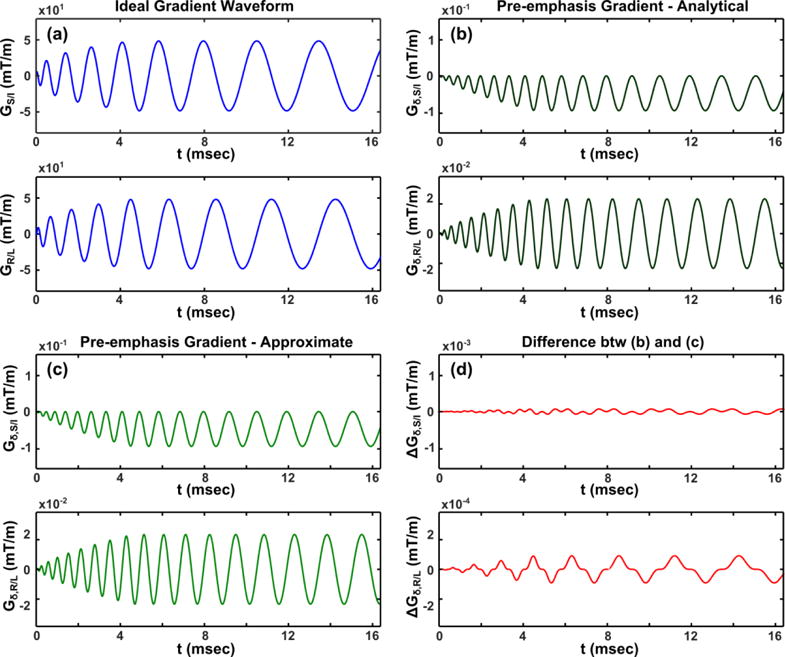
a: Gradient waveforms of a 2D coronal spiral acquisition; b, c: pre-emphasized gradient waveform component for first-order concomitant field correction obtained from closed-form analytical solution (b), and the approximate solution (c); d: the difference between the analytical and approximate solutions. Note the y-axis scale changes among figures.

The phase maps reconstructed from the phase-difference data acquired with the nominal and pre-emphasized gradient waveforms are shown in Fig. 3. A retrospectively corrected phase map by removing the phase accumulation due to concomitant field is also shown. Line profiles across the phase images are also demonstrated. The effects of the first-order concomitant fields generated by the asymmetric gradient, which manifest as a linear phase accumulation across the phase image, is apparent in the image generated from data acquired using the nominal gradient waveforms. Comparatively, these phase errors are virtually eliminated in the images generated from data acquired using the proposed pre-emphasized gradients. The small residual errors after pre-emphasis are most likely due to residual eddy currents. Table 2 summarizes the slopes of the line profiles in Fig. 3 obtained from linear regression analysis. The linear phase variation as represented by the slope of line profile is largely reduced using the proposed gradient pre-emphasis method. Figure 3 and Table 2 also show that the proposed gradient pre-emphasis method can prospectively account for the effect of concomitant fields, yielding equivalent results to retrospective correction but without the need for altering the image reconstruction process.

Figure 3.

Phase images reconstructed from phase-contrast-like acquisitions (121 gradient amplitude = 72 mT/m, slew rate = 700 T/m/sec) using gradient waveforms before (a to c) and after (d to f) the proposed first-order concomitant field (CF) gradient pre-emphasis method. g to i: phase images obtained after applying retrospective phase correction to a to c. The first-order concomitant fields introduce a linear phase variation across the phantom, which is mitigated by the gradient pre-emphasis. The small residual phase is most likely due to residual gradient eddy-currents.

Table 2.

Slope of the line profiles shown in Figure 3.

	Slope of Line Profiles (rad per pixel)
Acquisition Plane	Axial	Coronal	Sagittal
Before CF Pre-Emphasis	−0.0641	−0.1371	0.1355
After CF Pre-Emphasis	0.0013	0.0031	−0.0036
Retrospective Correction	0.0030	0.0052	−0.0062

Phantom images at different slice locations reconstructed from axial spiral data acquired with and without gradient pre-emphasis are shown in Fig. 4. The image obtained from retrospective reconstruction-based correction is also shown as a reference. Note that the first-order concomitant fields introduce considerable distortion. The concomitant field for this axial spiral acquisition causes phase accumulation with first-order spatial dependence along the slice selection direction (gradient z-axis), which causes its effect to vary among slice locations, as shown in Figs. 4a and 4b. Figs. 4c and 4d demonstrate that applying the proposed gradient pre-emphasis greatly reduces these artifacts. For example, in Figs 4b and 4d, the full width half maximum (FWHM) of the line plot is reduced from 3.04 to 1.64 mm, representing a substantial increase in sharpness. Comparison between Figs. 4e and 4f show that prospectively accounting for the effect of concomitant field using the proposed gradient pre-emphasis method yields equivalent results to retrospective reconstruction-based correction. However, modification of the reconstruction process is not required for the proposed pre-emphasis method.

Figure 4.

Phantom images (and line profiles) reconstructed from axial spiral acquisition (spiral readout with maximum gradient amplitude of 49 mT/m and slew rate of 700 T/m/sec) before (a, b) and after (c, d) the proposed concomitant field (CF) gradient pre-emphasis. e and f: images obtained after applying retrospective reconstruction-based concomitant field correction to a and b. The concomitant fields cause image blurring and artifacts (a, b) dependent on slice locations (see Results for further discussion), which are greatly reduced after the proposed gradient pre-emphasis (c, d).

The coronal and sagittal spiral images (full scale and magnified inserts) acquired with and without the proposed gradient pre-emphasis are shown in Fig. 5, as well as the image obtained from retrospective reconstruction based concomitant field correction. Spatially varying blurring due to unaccounted concomitant field-induced phase in the measured MRI data can be observed at the superior end of the phantom images (Figs. 5a and 5d). As shown in Fig. 5, both the proposed gradient pre-emphasis strategy and the reconstruction based correction successfully prevent these spurious effects.

Figure 5.

Phantom images (full scale and magnified inserts) reconstructed from coronal (a, b) and sagittal (d, e) spiral acquisitions (spiral readout with maximum gradient amplitude of 49 mT/m and slew rate of 700 T/m/sec) before (a, d) and after (b, e) the proposed concomitant field (CF) gradient pre-emphasis. c and f: images obtained after applying retrospective reconstruction based concomitant field correction to a and d. The spatially dependent blurring apparent at the superior ends of the images (a, d, also see magnified inserts and line profiles) is absent in images acquired with the proposed pre-emphasized gradients (b, e).

Figure 6 shows axial brain images acquired using the nominal and pre-emphasized spiral gradient waveforms, which demonstrates the spatial blurring introduced by the first-order concomitant fields. Note the blurring of small cortical arteries (red arrows) and vein (blue arrow), and artifactual distortion and enlargement of vessels in Fig. 6a. Fig. 6b demonstrates that the described method effectively reduces blurring and enables clearer depiction of small structures, like the small cortical arteries and vein. Fig. 6c shows the image obtained after applying retrospective reconstruction based concomitant field correction to Fig. 6a, where a similar level of compensation can be observed.

Figure 6.

Brain scan examples of a 2D axial spiral acquisition (spiral readout with maximum gradient amplitude of 33 mT/m and slew rate of 700 T/m/sec) using the nominal (a) and concomitant field (CF) pre-emphasized (b) gradient waveforms. c: images obtained after applying retrospective reconstruction based concomitant field correction to a. Note the blurring of small cortical arteries (red arrows) and vein (blue arrow) caused by unaccounted first-order concomitant fields (a). The proposed CF gradient pre-emphasis method successfully prevents this degradation (b).

The 2D axial EPI image series acquired with gradient waveforms before and after the proposed gradient pre-emphasis are reformatted in a sagittal plane and shown in Figs. 7a and 7b. Examples of axial images acquired at S/I = 8.5 cm before (Fig. 7c) and after (Fig. 7d) gradient pre-emphasis are also shown. The first-order concomitant field causes an image shift along the anterior/posterior gradient axis (phase encoding direction) as shown in Fig. 7a and indicated by the red arrow in Fig. 7c. Note that this image shift causes the image-domain based gradient nonlinearity correction on scanner to misregister image content at inaccurate physical positions, leaving observable residual geometric distortion in corrected images (see the green arrow in Fig. 7c). As shown in Figs. 7b and 7d, prospectively accounting for its effect using the gradient pre-emphasis method prevents this image shift, and reduces the residual image distortion after gradient nonlinearity correction. The residual image shift at the superior and inferior ends of the phantom in Figs. 7b and 7d is likely due to B₀ inhomogeneity and susceptibility effects.

Figure 7.

Phantom images of a 2D axial multi-slice EPI acquisition (EPI readout with maximum gradient amplitude of 41 mT/m and slew rate of 700 T/m/sec) before and after the proposed first-order concomitant field (CF) gradient pre-emphasis. a and b: Sagittal reformat of the 2D axial image series before (a) and after (b) CF gradient pre-emphasis. c and d: Example of axial images (slice SI position = 8.5 cm) before (c) and after (d) CF gradient pre-emphasis (positions are marked as red dashed lines in the sagittal reformat). The proposed pre-emphasis method prevents the image shift along the anterior/posterior gradient axis (a vs b, also see red arrows), and reduce the residual image geometric distortion caused by inaccurate image domain gradient nonlinearity correction due to this shift (green arrows).

DISCUSSION

In this work, we have developed a real-time gradient pre-emphasis strategy that simultaneously counteracts all the first-order concomitant fields on asymmetric gradient systems for any arbitrary gradient waveform. A numerically straightforward, simple to implement approximate solution was derived and directly implemented on the same hardware infrastructure that prospective eddy current compensation was performed. The ideal gradient waveforms are taken as input, along with system-specific parameters like $B_0$ and $z_0$, and this hardware then calculates pre-emphasized gradients using simple, arithmetic operations. The results of a series of phantom and in vivo scans using Cartesian phase-difference, EPI, and spiral acquisitions indicate that the first-order concomitant fields, if not properly accounted for, cause considerable phase estimation error, image shift, blurring and ghosting. Those artifacts can be effectively eliminated with the proposed method (Figs. 3 to 7).

The proposed gradient pre-emphasis method can potentially benefit any MR data acquisition performed on the asymmetric gradient system. This method may be particularly helpful for imaging 3D volumes acquired for arterial spin labeling applications that use stacks of spiral acquisitions (30), 3D radial acquisition (31), and shells with integrated radial and spiral (SWIRLS) (32). Note that Eq. 6 predicts that the effects of the first-order concomitant fields increase as the imaging region is farther displaced from gradient isocenter, highlighting the importance of its compensation. As concomitant field strength scales with gradient amplitude squared, the proposed pre-emphasis strategy will also benefit MR acquisitions employing multiple large gradient lobes, such as EPI-based sequences and small FOV applications. Because the concomitant fields scale inversely with the main field strength B₀, all the deleterious effects described here would be doubled at 1.5 T compared to the 3.0 T results shown here.

Due to their same linear spatial dependence and similar image artifact manifestation, the linear concomitant fields can potentially be confused with linear gradient eddy currents, which are typically characterized using a separate calibration procedure (33,34). Hence, prospective counteraction of concomitant field effects can eliminate this potentially confounding factor and improve the accuracy of gradient eddy current calibration on asymmetric gradient systems. Eddy current pre-emphasis was performed during data acquisition. One limitation of this study is that the eddy current calibration process did not include concomitant field compensation. Similarly, prospective, real-time compensation of the zeroth-order concomitant fields using the methods of Ref. (17) is expected to remove another confounding factor in B₀ eddy-current calibration. We are currently developing a real-time implementation of the zeroth-order concomitant field compensation, and plan to report those results in future work.

The proposed gradient pre-emphasis strategy can be readily incorporated into the current MR system workflow. It can be implemented either in the pulse sequence or hardware (e.g., eddy current pre-emphasis firmware), offering substantial implementation flexibility. When implemented in hardware, it can be performed together with gradient eddy current pre-emphasis, as done in this work, and therefore is transparent to pulse sequence design or subsequent corrections of off resonance (27), gradient delays, eddy currents (35,36), gradient nonlinearity (22,26,37), or second-order concomitant fields (1,3–5). Note that simultaneous correction during image reconstruction of off-resonance, gradient nonlinearity, and second-order concomitant fields were demonstrated in our experimental results. If gradient pre-emphasis is implemented in the gradient driver firmware, any logical-to-physical translation of gradient axes (6) will be performed automatically, as in the results reported here. Alternatively, if the pre-emphasis is performed on host computer by modifying the pulse sequence, then the logical-to-physical translation of gradient axes must be accounted for, which is considerably less convenient.

The approximate solution described in Eq. 9 was derived from a general asymmetric gradient model (Eq. 8) assuming arbitrary asymmetry parameters ( $x_0$, $y_0$, $z_{0x}$, $z_{0y}$, $\alpha$). Therefore, this method is general and could be applied to other asymmetric gradient systems, such as that reported in a previous work (12), or systems with new designs developed in the future.

CONCLUSIONS

A gradient pre-emphasis method suitable for real-time implementation was developed to provide flexible and effective counteraction of image artifacts from the first-order concomitant fields that are specific to asymmetric gradient systems. The feasibility of the method was demonstrated in phantom and human tests. The proposed method is general, and can be applied to a variety of acquisition strategies and arbitrary gradient waveforms. When implemented alongside the linear eddy-current compensation as reported here, no pulse sequence modifications are required, and the logical-to-physical translations are handled automatically.

APPENDIX A

Here we show the derivation of Eq. 9 from Eq. 8. Rearranging Eq. 8 yields:

$$G_x^0=G_x-\frac{{\alpha }^2{\left(G_z^0\right)}^2{x}_0}{B_0}+\frac{\alpha G_x^0{G}_z^0{z}_{0x}}{B_0}$$ (A1.a)

$$G_y^0=G_y-\frac{{\left(1-\alpha \right)}^2{\left(G_z^0\right)}^2{y}_0}{B_0}+\frac{\left(1-\alpha \right)G_y^0{G}_z^0{z}_{0y}}{B_0}$$ (A1.b)

$$G_z^0=G_z-\frac{{\left(G_x^0\right)}^2{z}_{0x}}{B_0}-\frac{{\left(G_y^0\right)}^2{z}_{0y}}{B_0}+\frac{\alpha G_x^0{G}_z^0{x}_0}{B_0}+\frac{\left(1-\alpha \right)G_y^0{G}_z^0{y}_0}{B_0}$$ (A1.c)

The expressions for $G_x^0$, $G_y^0$, $G_z^0$ in Eq. A1 include $G_x$, $G_y$, and $G_z$, as well as higher order terms including ${\left(G_x^0\right)}^2$, ${\left(G_y^0\right)}^2$, ${\left(G_z^0\right)}^2$, $G_x^0{G}_z^0$, and $G_y^0{G}_z^0$ on the right side, thus the applied waveforms will be fixed points of this nonlinear system of equations ( ${\mathbf{G}}^0=f\left({\mathbf{G}}^0\right)$). Note that the expansions of ${\left(G_x^0\right)}^2$, ${\left(G_y^0\right)}^2$, ${\left(G_z^0\right)}^2$, $G_x^0{G}_z^0$, and $G_y^0{G}_z^0$ with respect to $G_x$, $G_y$, and $G_z$ will contain only second-order terms of $G_x$, $G_y$, $G_z$ and even higher-order terms. Therefore, the second-order approximation of Eq. A1 with respect to $G_x$, $G_y$, and $G_z$ yields:

$$G_x^0=G_x-\frac{{\alpha }^2{\left(G_z\right)}^2{x}_0}{B_0}+\frac{\alpha G_x{G}_z{z}_{0x}}{B_0}+o\left({\displaystyle \sum _{m,n,p=x,y,z}\frac{G_m{G}_n{G}_p}{{\left(B_0\right)}^2}{r}^2}\right)$$ (A2.a)

$$G_y^0=G_y-\frac{{\left(1-\alpha \right)}^2{\left(G_z\right)}^2{y}_0}{B_0}+\frac{\left(1-\alpha \right)G_y{G}_z{z}_{0y}}{B_0}+o\left({\displaystyle \sum _{m,n,p=x,y,z}\frac{G_m{G}_n{G}_p}{{\left(B_0\right)}^2}{r}^2}\right)$$ (A2.b)

$$G_z^0=G_z-\frac{{\left(G_x^0\right)}^2{z}_{0x}}{B_0}-\frac{{\left(G_y^0\right)}^2{z}_{0y}}{B_0}+\frac{\alpha G_x^0{G}_z^0{x}_0}{B_0}+\frac{\left(1-\alpha \right)G_y^0{G}_z^0{y}_0}{B_0}+o\left({\displaystyle \sum _{m,n,p=x,y,z}\frac{G_m{G}_n{G}_p}{{\left(B_0\right)}^2}{r}^2}\right)$$ (A2.c)

where $r=max\left\{x_0,y_0,z_{0x},z_{0y}\right\}$. Ignoring the higher order ( $\ge 3$) in Eq. A2 yields Eq. 9. Solutions shown in Eq. 9 can also be considered as the first-iteration approximation of a fixed-point iteration solver initialized with ideal gradient waveforms $G_x$, $G_y$, and $G_z$, which reveals itself by inserting $G_x^0=G_x$, $G_y^0=G_y$, and $G_z^0=G_z$ into the right side of Eq. A1. Figure 8 shows the monotonic decrease of residual errors at each iteration for solving the gradient pre-emphasis problem (Eq. A1) using the fixed-point iteration method ( ${\mathbf{G}}^0=f\left({\mathbf{G}}^0\right)$). Note that the residual error quickly drops to the machine precision level, showing convergence of fixed-point iteration.

Figure 8.

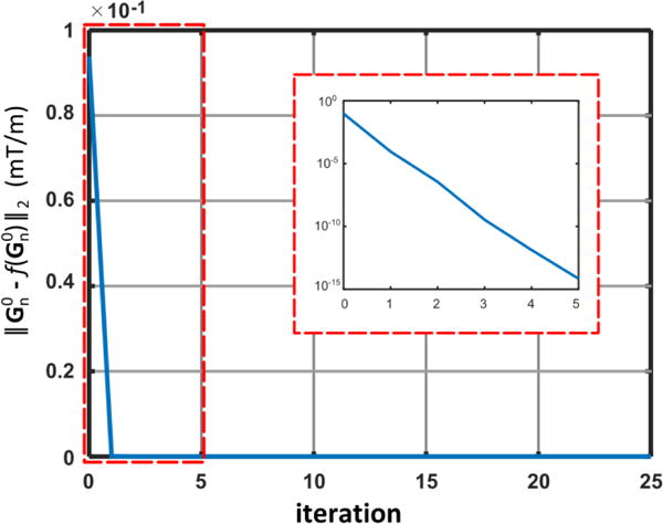
Convergence curve showing the progressive decrease of residual error ( ${\Vert {\mathbf{G}}_n^0-f\left({\mathbf{G}}_n^0\right)\Vert }_2$) at each fixed-point iteration ( $f\left({\mathbf{G}}_n^0\right)={\mathbf{G}}_n^0$) used to exactly solve the gradient pre-emphasis problem (Eq. A1). The zoom-in panel shows (log-scale) the residual errors of the first 5 iterations, which quickly drops to the machine precision level of the gradient firmware. Note that the first iteration corresponds to the approximate solution in Eq. 9. The very small residual error after the first iteration supports the use of this value as an approximate solution of the gradient pre-emphasis calculation problem.

APPENDIX B

In this appendix, we demonstrate that the closed-form, analytical solution to the exact gradient pre-emphasis scheme (Eq. 11) exists for the gradient system with equivalent asymmetric transverse gradient and symmetric z gradient. Inserting system offset parameters: $x_0=0$, $y_0=0$, $z_{0x}=z_{0y}=z_0$, and $\alpha =0.5$ into Eq. 8 yields:

$$G_x=G_x^0-\frac{G_x^0{G}_z^0{z}_0}{2B_0}$$ (B1.a)

$$G_y=G_y^0-\frac{G_y^0{G}_z^0{z}_0}{2B_0}$$ (B1.b)

$$G_z=G_z^0+\frac{{\left(G_x^0\right)}^2{z}_0}{B_0}+\frac{{\left(G_y^0\right)}^2{z}_0}{B_0}$$ (B1.c)

The systems of equations in Eq. B1 can be combined as a cubic equation of $G_z^0$ with real-valued coefficients:

$$a_1{\left(G_z^0\right)}^3+a_2{\left(G_z^0\right)}^2+a_3{G}_z^0+a_4=0$$ (B2)

where $a_1=z_0^2/4$, $a_2=-G_z{z}_0^2/4-B_0{z}_0$, $a_3=B_0{z}_0{G}_z+B_0^2$, $a_4=-B_0^2{G}_z+B_0{z}_0\left(G_x^2+G_y^2\right)$. The above cubic equation has at least one real-valued solution (38), which can be written as:

$$G_z^0=-\frac{1}{3a_1}\left(a_2+A+\frac{{\mathrm{\Delta }}_0}{A}\right)$$ (B3.a)

where $A=\sqrt[3]{\left({\mathrm{\Delta }}_1+\sqrt{{\mathrm{\Delta }}_1^2-4{\mathrm{\Delta }}_0^3}\right)/2}$, ${\mathrm{\Delta }}_0=a_2^2-3a_1{a}_3$, ${\mathrm{\Delta }}_1=2a_2^3-9a_1{a}_2{a}_3+27a_1^2{a}_4$. Eq. (B3.a) gives the expression of z gradient waveform after pre-emphasis based on ideal/target gradient waveforms. Rearranging Eqs. (B1.a) and (B1.b) then gives:

$$G_x^0=\frac{B_0{G}_x}{B_0-G_z^0{z}_0/2}$$ (B3.b)

$$G_y^0=\frac{B_0{G}_y}{B_0-G_z^0{z}_0/2}$$ (B3.c)

which describes the pre-emphasized x and y gradients using Eq. B3.a.

References

- 1.Bernstein MA, Zhou XJ, Polzin JA, King KF, Ganin A, Pelc NJ, Glover GH. Concomitant gradient terms in phase contrast MR: analysis and correction. Magn Reson Med. 1998;39:300–308. doi: 10.1002/mrm.1910390218. [DOI] [PubMed] [Google Scholar]
- 2.Norris DG, Hutchison JMS. Concomitant magnetic field gradients and their effects on imaging at low magnetic field strengths. Magn Reson Imaging. 1990;8:33–37. doi: 10.1016/0730-725x(90)90209-k. [DOI] [PubMed] [Google Scholar]
- 3.King KF, Ganin A, Zhou XJ, Bernstein MA. Concomitant gradient field effects in spiral scans. Magn Reson Med. 1999;41:103–112. doi: 10.1002/(sici)1522-2594(199901)41:1<103::aid-mrm15>3.0.co;2-m. [DOI] [PubMed] [Google Scholar]
- 4.Du YP, Zhou XJ, Bernstein MA. Correction of concomitant magnetic field-induced image artifacts in nonaxial echo-planar imaging. Magn Reson Med. 2002;48:509–515. doi: 10.1002/mrm.10249. [DOI] [PubMed] [Google Scholar]
- 5.Zhou XJ, Du YP, Bernstein MA, Reynolds HG, Maier JK, Polzin JA. Concomitant magnetic-field-induced artifacts in axial echo planar imaging. Magn Reson Med. 1998;39:596–605. doi: 10.1002/mrm.1910390413. [DOI] [PubMed] [Google Scholar]
- 6.Bernstein MA, King KF, Zhou XJ. Handbook of MRI pulse sequences. Burlington: Elsevier Academic Press; 2004. [Google Scholar]
- 7.Zhou XJ, Tan SG, Bernstein MA. Artifacts induced by concomitant magnetic field in fast spin-echo imaging. Magn Reson Med. 1998;40:582–591. doi: 10.1002/mrm.1910400411. [DOI] [PubMed] [Google Scholar]
- 8.Cheng JY, Santos JM, Pauly JM. Fast concomitant gradient field and field inhomogeneity correction for spiral cardiac imaging. Magn Reson Med. 2011;66:390–401. doi: 10.1002/mrm.22802. [DOI] [PMC free article] [PubMed] [Google Scholar]
- 9.Alsop DC, Connick TJ. Optimization of torque-balanced asymmetric head gradient coils. Magn Reson Med. 1996;35:875–886. doi: 10.1002/mrm.1910350614. [DOI] [PubMed] [Google Scholar]
- 10.Chronik BA, Alejski A, Rutt BK. Design and fabrication of a three-axis edge ROU head and neck gradient coil. Magn Reson Med. 2000;44:955–963. doi: 10.1002/1522-2594(200012)44:6<955::aid-mrm18>3.0.co;2-1. [DOI] [PubMed] [Google Scholar]
- 11.Roemer PB, inventors, General Electric Company, assignee Transverse gradient coils for imaging the head. 5,177,442. US Patent. 1993 Jan 5;
- 12.Meier C, Zwanger M, Feiweier T, Porter D. Concomitant field terms for asymmetric gradient coils: consequences for diffusion, flow, and echo-planar imaging. Magn Reson Med. 2008;60:128–134. doi: 10.1002/mrm.21615. [DOI] [PubMed] [Google Scholar]
- 13.Lee SK, Mathieu JB, Graziani D, Piel J, Budesheim E, Fiveland E, Hardy CJ, Tan ET, Amm B, Foo TK, Bernstein MA, Huston J, 3rd, Shu Y, Schenck JF. Peripheral nerve stimulation characteristics of an asymmetric head-only gradient coil compatible with a high-channel-count receiver array. Magn Reson Med. 2015 doi: 10.1002/mrm.26044. [DOI] [PMC free article] [PubMed] [Google Scholar]
- 14.Kickler N, van der Zwaag W, Mekle R, Kober T, Marques JP, Krueger G, Gruetter R. Eddy current effects on a clinical 7T-68 cm bore scanner. Magn Reson Mater Phy. 2010;23:39–43. doi: 10.1007/s10334-009-0192-0. [DOI] [PubMed] [Google Scholar]
- 15.O’Brien KR, Kober T, Hagmann P, Maeder P, Marques J, Lazeyras F, Krueger G, Roche A. Robust T1-weighted structural brain imaging and morphometry at 7T using MP2RAGE. PloS one. 2014;9:e99676. doi: 10.1371/journal.pone.0099676. [DOI] [PMC free article] [PubMed] [Google Scholar]
- 16.vom Endt A, Riegler J, Eberlein E, Schmitt F, Dorbert U, Krüger G, Gruetter R. A high-performance head gradient coil for 7T systems. Proceedings of the 15th annual meeting of the ISMRM; Berlin, Germany. 2007. p. 451. [Google Scholar]
- 17.Crozier S, Eccles CD, Beckey FA, Field J, Doddrell DM. Correction of eddy-current-induced B0 shifts by receiver reference-phase modulation. J Magn Reson. 1992;97:661–665. [Google Scholar]
- 18.Tao S, Trzasko JD, Shu Y, Weavers PT, Lee S-K, Bernstein MA. Closed-form solution concomitant field correction method for echo planar imaging on head-only asymmetric gradient. Proceedings of the 23rd annual meeting of the ISMRM; Toronto, Canada. 2015. p. 3776. [Google Scholar]
- 19.Phantom test guidance for the ACR MRI accreditation program. Reston: The American College of Radiology; Reston, Virginia: 2005. [Google Scholar]
- 20.King KF, Foo TK, Crawford CR. Optimized gradient waveforms for spiral scanning. Magn Reson Med. 1995;34:156–160. doi: 10.1002/mrm.1910340205. [DOI] [PubMed] [Google Scholar]
- 21.Site scanning instructions for use of the small MR phantom for the ACR MRI accreditation program. Reston: The American College of Radiology; Reston, Virginia: 2008. [Google Scholar]
- 22.Tao S, Trzasko JD, Shu Y, Huston J, 3rd, Bernstein MA. Integrated image reconstruction and gradient nonlinearity correction. Magn Reson Med. 2015;74:1019–1031. doi: 10.1002/mrm.25487. [DOI] [PMC free article] [PubMed] [Google Scholar]
- 23.Bernstein MA, Ikezaki Y. Comparison of phase-difference and complex-difference processing in phase-contrast MR angiography. J Magn Reson Imaging. 1991;1:725–729. doi: 10.1002/jmri.1880010620. [DOI] [PubMed] [Google Scholar]
- 24.Beatty PJ, Nishimura DG, Pauly JM. Rapid gridding reconstruction with a minimal oversampling ratio. IEEE Trans Med Imaging. 2005;24:799–808. doi: 10.1109/TMI.2005.848376. [DOI] [PubMed] [Google Scholar]
- 25.Fessler JA, Sutton BP. Nonuniform fast Fourier transforms using min-max interpolation. IEEE Trans Signal Proces. 2003;51:560–574. [Google Scholar]
- 26.Tao S, Trzasko JD, Shu Y, Huston J, 3rd, Johnson KM, Weavers PT, Gray EM, Bernstein MA. NonCartesian MR image reconstruction with integrated gradient nonlinearity correction. Med Phys. 2015;42:7190. doi: 10.1118/1.4936098. [DOI] [PMC free article] [PubMed] [Google Scholar]
- 27.Noll DC, Meyer CH, Pauly JM, Nishimura DG, Macovski A. A homogeneity correction method for magnetic resonance imaging with time-varying gradients. IEEE Trans Med Imaging. 1991;10:629–637. doi: 10.1109/42.108599. [DOI] [PubMed] [Google Scholar]
- 28.Funai AK, Fessler JA, Yeo DT, Olafsson VT, Noll DC. Regularized field map estimation in MRI. IEEE Trans Med Imaging. 2008;27:1484–1494. doi: 10.1109/TMI.2008.923956. [DOI] [PMC free article] [PubMed] [Google Scholar]
- 29.Kolmogorov V, Zabih R. What energy functions can be minimized via graph cuts? IEEE Trans Pattern Anal and Mach Intell. 2004;26:147–159. doi: 10.1109/TPAMI.2004.1262177. [DOI] [PubMed] [Google Scholar]
- 30.Dai W, Garcia D, de Bazelaire C, Alsop DC. Continuous flow-driven inversion for arterial spin labeling using pulsed radio frequency and gradient fields. Magn Reson Med. 2008;60:1488–1497. doi: 10.1002/mrm.21790. [DOI] [PMC free article] [PubMed] [Google Scholar]
- 31.Johnson KM, Lum DP, Turski PA, Block WF, Mistretta CA, Wieben O. Improved 3D phase contrast MRI with off-resonance corrected dual echo VIPR. Magn Reson Med. 2008;60:1329–1336. doi: 10.1002/mrm.21763. [DOI] [PMC free article] [PubMed] [Google Scholar]
- 32.Shu Y, Bernstein MA, Huston J, 3rd, Rettmann D. Contrast-enhanced intracranial magnetic resonance angiography with a spherical shells trajectory and online gridding reconstruction. J Magn Reson Imaging. 2009;30:1101–1109. doi: 10.1002/jmri.21938. [DOI] [PubMed] [Google Scholar]
- 33.Jehenson P, Westphal M, Schuff N. Analytical method for the compensation of eddy-current effects induced by pulsed magnetic-field gradients in NMR systems. J Magn Reson. 1990;90:264–278. [Google Scholar]
- 34.Van Vaals JJ, Bergman AH. Optimization of eddy-current compensation. J Magn Reson. 1990;90:52–70. [Google Scholar]
- 35.Brodsky EK, Samsonov AA, Block WF. Characterizing and correcting gradient errors in non-cartesian imaging: are gradient errors linear time-invariant (LTI)? Magn Reson Med. 2009;62:1466–1476. doi: 10.1002/mrm.22100. [DOI] [PMC free article] [PubMed] [Google Scholar]
- 36.Tan H, Meyer CH. Estimation of k-space trajectories in spiral MRI. Magn Reson Med. 2009;61:1396–1404. doi: 10.1002/mrm.21813. [DOI] [PMC free article] [PubMed] [Google Scholar]
- 37.Glover GH, Pelc NJ, inventors, General Electric Company, assignee Method for correcting image distortion due to gradient nonuniformity. 4,591,789. US Patent. 1986 May 27;
- 38.Press W, Teukolsky S, Vetterling W, Flannery B. Numerical recipes in Fortran 77: the art of scientific computing. New York, NY: Cambridge University Press; 1992. [Google Scholar]