

A new Bayesian photobleaching trace analysis method that is computationally inexpensive can be used to treat blinking, reactivation, and overlapping events and reliably detect up to 50 fluorophores even for low signal-to-noise ratios. It can also scale up to 500+ for high signal-to-noise ratios.
Abstract
Photobleaching event counting is a single-molecule fluorescence technique that is increasingly being used to determine the stoichiometry of protein and RNA complexes composed of many subunits in vivo as well as in vitro. By tagging protein or RNA subunits with fluorophores, activating them, and subsequently observing as the fluorophores photobleach, one obtains information on the number of subunits in a complex. The noise properties in a photobleaching time trace depend on the number of active fluorescent subunits. Thus, as fluorophores stochastically photobleach, noise properties of the time trace change stochastically, and these varying noise properties have created a challenge in identifying photobleaching steps in a time trace. Although photobleaching steps are often detected by eye, this method only works for high individual fluorophore emission signal-to-noise ratios and small numbers of fluorophores. With filtering methods or currently available algorithms, it is possible to reliably identify photobleaching steps for up to 20–30 fluorophores and signal-to-noise ratios down to ∼1. Here we present a new Bayesian method of counting steps in photobleaching time traces that takes into account stochastic noise variation in addition to complications such as overlapping photobleaching events that may arise from fluorophore interactions, as well as on-off blinking. Our method is capable of detecting ≥50 photobleaching steps even for signal-to-noise ratios as low as 0.1, can find up to ≥500 steps for more favorable noise profiles, and is computationally inexpensive.
INTRODUCTION
Fluorophores photobleach when exposed to light over time. That is, they irreversibly photochemically transition to a state no longer detectable by fluorescence (White and Stelzer, 1999; Lippincott-Schwartz et al., 2003). Although photobleaching can be a nuisance in single-particle tracking experiments, it is critical to other experimental approaches, such as fluorescence recovery after photobleaching (Lippincott-Schwartz et al., 2003), photoactivated localization microscopy (PALM), and photobleaching event counting (Lippincott-Schwartz et al., 2003; Leake et al., 2006; Ulbrich and Isacoff, 2007; Coffman and Wu, 2012). As its name implies, photobleaching event counting is used to enumerate molecules by monitoring how the light intensity in some region decreases by quanta as individual fluorophores photobleach (Shu et al., 2007). This can be very useful in quantifying the stoichiometry of biological complexes in live cells (Leake et al., 2006).
Briefly, photobleaching event counting works by tagging biomolecule subunits—often genetically (Durisic et al., 2014)—with fluorophores. Fluorophores within an illuminated region of interest (ROI) are then all simultaneously activated and monitored as they subsequently photobleach. As each fluorophore photobleaches, the fluorescence intensity over a ROI drops in a step-like pattern. Each step-like decrease corresponds to a single or possibly multiple overlapping photobleaching events. The total number of photobleaching events can then be used, in principle, to determine the total number of fluorophore-tagged molecules present within the ROI (Das et al., 2007).
For instance, photobleaching event counting has been used to quantify the stoichiometry of a number of complexes involved in the bacterial flagellar switch (FliM; Delalez et al., 2010), eukaryotic flagella (Engel et al., 2009), and the point centromere (Lawrimore et al., 2011; Coffman et al., 2011). It also has been used to determine the stoichiometry of complexes and biomolecules such as mammalian neurotransmitter receptors (McGuire et al., 2012), human calcium channels (Demuro et al., 2011), transmembrane α-amino-3-hydroxy-5-methyl-4-isoxazolepropionic acid receptor-regulatory proteins (Hastie et al., 2013), T4 bacteriophage helicase loader protein (Arumugam et al., 2009), bacterial oxidative phosphorylation complexes (Llorente-Garcia et al., 2014), microRNAs in processing bodies (Pitchiaya et al., 2012, 2014), RNAs in a bacteriophage DNA-packaging motor (Shu et al., 2007), and other membrane protein and protein complex stoichiometries (Leake et al., 2006; Das et al., 2007).
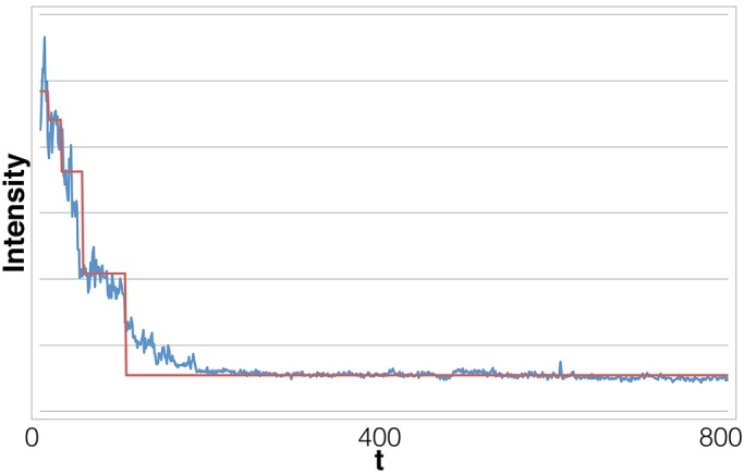
Although counting photobleaching steps is conceptually straightforward, the noise inherent to photobleaching traces makes it difficult to identify the number of steps and their location (Figure 1). One key challenge is that the magnitude of the noise changes stochastically along with the number of active fluorophores. Thus a detection algorithm assuming constant noise properties is inappropriate for photobleaching.
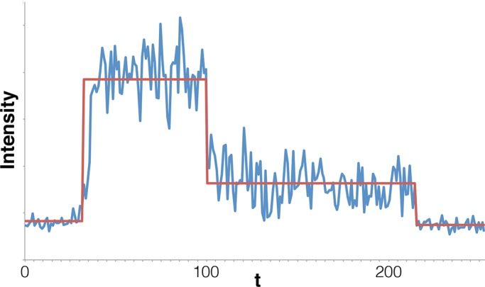
FIGURE 1:
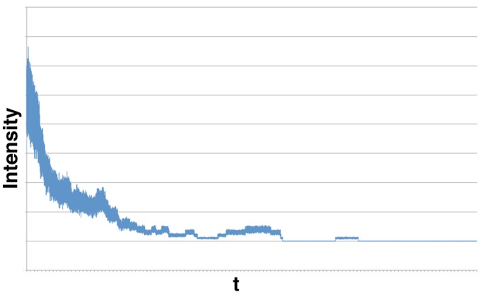
Synthetic photobleaching time trace for 50 fluorophores, with μf /σf = 10 for the single fluorophore, illustrating how noise obscures steps when many fluorophores are active at the start of the trace. Although it is easy to resolve individual steps late in the trace when fluorophore numbers are low, for >10 or so fluorophores, the steps are strongly obscured by additive noise. Here μf = 2.0, σf = 0.2, μb = 20.0, and σb = 0 (quantities defined in the text). Both time and fluorescence intensity are in arbitrary units.
In addition, noise also arises from background fluorescence (Ulbrich and Isacoff, 2007; Coffman and Wu, 2012), variable fluorophore emission (Ulbrich and Isacoff, 2007), and fluorophore blinking (Bagshaw and Cherny, 2006) driven by core fluorophore instabilities (Drobizhev et al., 2012). For this reason, photobleaching event counting is typically used only in systems with few fluorophores (<10), for which signal-to-noise ratio (SNR) is high. Here SNR is defined as μf/σf, where μf and σf are the mean and SD of the emission intensity of the single fluorophore, respectively. For instance, in Ulbrich and Isacoff (2007), five subunits was the limit past which detection of discrete steps, done by eye, became difficult. Figure 1 shows an example of a photobleaching trace along with its increasing noise level as more fluorophores become active.
Earlier counting methods used filters—such as the median filter or the Chung–Kennedy filter (Leake et al., 2006)—as well as binning and constructing pairwise distance distributions (Svoboda et al., 1993) and other techniques (Coffman and Wu, 2012) and were able to count ∼10 steps. With more recent step-finding algorithms (Kerssemakers et al., 2006; Kalafut and Visscher, 2008; Carter et al., 2008), the number of detectable steps increases to ∼15–30 (Das et al., 2007; Engel et al., 2009; Coffman and Wu, 2012).
The latest approaches—relying on the Schwarz information criterion (SIC; also sometimes called the Bayesian information criterion; Schwarz, 1978; Chen et al., 2014) and the Student’s two-sample t test (Chen et al., 2014)—encounter problems for >20 steps and SNR < 2. Although SIC and Student’s t-test algorithms improve how many steps may be detected, visual inspection, supplemented by filtering methods, is still often used (Engel et al., 2009).
One shortcoming of these previous methods is that they do not directly account for on-off blinking or stochastically varying noise. Here we present a Bayesian approach to counting that directly addresses the foregoing challenges. Conceptually, our method uses a likelihood function that is adapted to treat the physics of the noise properties expected in photobleaching and introduces a prior that corrects for systematic biases that would otherwise arise from simple likelihood maximization.
Brute-force application of many methods, including our own, that rank-order models by evaluating and comparing model posteriors for all possible models (i.e., all possible numbers of steps with any possible step location) is computationally prohibitive. Instead, our method is efficient in its implementation because it uses a precursor algorithm to eliminate from consideration a large number of unlikely models. It then considers and compares only probable models.
This two-step approach reduces the computational complexity and makes it possible for us to apply our method to photobleaching traces with as many as 100+ fluorophores, depending on the level of noise. In fact, using our method, we show that even for low SNR, we can count up to 50+ fluorophores and locate photobleaching events in a time trace with an accuracy surpassing that of methods currently available. We also show that we can extract biological conclusions by applying our method to sample experimental data sets.
We previously proposed a solution to the single-molecule counting problem using PALM (Rollins et al., 2015), in which we inferred the (stochastic) blinking properties of fluorophores “on the fly” in order to avoid overcounting fluorophores—and thus protein subunits—in an ROI. Although PALM provides greater spatial resolution than photobleaching event counting, allowing us to characterize complexes localized down to the tens of nanometers (Watanabe et al., 2011), PALM analysis is computationally intensive. The advantage of photobleaching, and the reason we focus on this here, is that photobleaching event counting has the potential to reveal the stoichiometry of complexes involving hundreds of proteins. Unfortunately, current analysis methods have limited its applicability to complexes with only a handful of subunits. As we show, complicated fluorophore photophysics can be accommodated in our approach. Thus our work even suggests that future experiments may want to focus on biological problems, such as characterizing larger protein complexes, rather than engineering photophysical properties of fluorophores used in photobleaching event counting to reduce blinking, which may now be treated theoretically in postprocessing.
METHODOLOGY
A brief sketch of our approach
A photobleaching time trace is a data set consisting of fluorescence intensity measurements taken at constant time intervals ∆t and ordered in sequence by ascending acquisition time. Traces are typically obtained when fluorophore-tagged molecules of interest are illuminated at some time, say t = 0, and then monitored until all fluorophores have photobleached. Photobleaching time traces present a model selection problem (Ludden et al., 1994; Cavanaugh and Neath, 1999; Stoica and Selen, 2004; Kalafut and Visscher, 2008; Pressé et al., 2013) for which a different number of steps and their locations within the trace, that is, the “model,” must be found.
Concretely, we use a Bayesian method to determine both the number of photobleaching steps, K, and their location in time, s = {s1, · · · , sK}. We call each possible {s, K} pair a model. Our method is implemented in a two-step algorithm intended to greatly reduce the computational requirements by eliminating from consideration a large number of unlikely models and thus limit the number of models whose relative merit (maximum marginal posterior) we must compare.
We benchmark our approach on synthetic data, demonstrating its applicability and limitations, and subsequently apply it to real experimental data. Our algorithm is implemented in a simple, freely available Python code on the corresponding author’s website.
A model selection criterion for photobleaching event counting
Any time there are i active fluorophores in a time trace, we say the trace is “visiting state i.” The total number of times state i is visited is Ji (which may be different from 1 if fluorophores blink). We label ϕij the jth interval—a collection of data points consecutive in time—during which the trace visits state i; see Figure 2 for a schematic representation.
FIGURE 2:
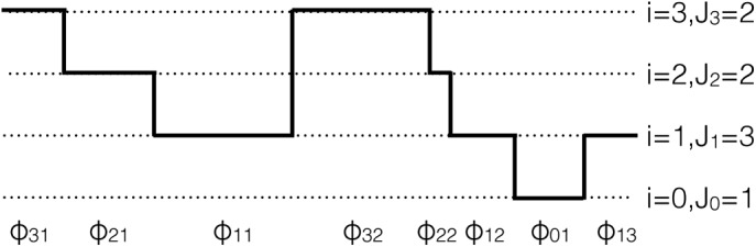
Schematic illustrating the variables used in Eq. 1. Idealized time trace with no noise. The number of active fluorophores, i, goes from 0 to 3, and so we have four states (0,1, 2, 3). The maximum number of fluorophores that can ever be active at the same time is three. Ji, the number of times the ith state is visited, ranges from 1 for i = 0 to 3 for i = 1; j runs from 1 to Ji for each i. There are eight ϕij intervals.
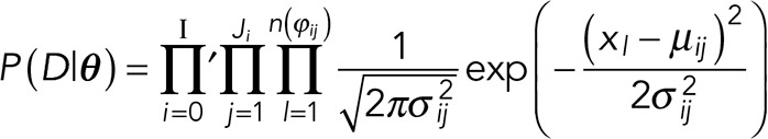
The likelihood of the data, D, given the model—whose parameters we collectively refer to as θ— is
 (1) (1)
|
Here I is the number of fluorophores initially present in the system; the number of active fluorophores can never exceed I. n(ϕij) is the number of data points in the ϕij interval. xl is the signal intensity at data point l, D = {xl}, and i iterates over the states, j over the number of visits to a particular state, and l over the number of data points in an interval. The mean and SD of the fluorescence intensity at the ϕij interval are μij and σi, respectively. The mean of any interval belonging to the ith state should take the form μij = μi = iμf + μb, and its variance should take the form σij2 = σi2 = iσf2 + σb2. In other words, the mean and variance of a particular interval depend only on the state (number of active fluorophores) i and not the number of times j that state is visited, and so we can drop j for notational simplicity. The quantities μf, σf, μb, and σb (where the subscript f designates single-fluorophore values and the subscript b designates background) are relatively easy to determine experimentally from the end of the photobleaching time trace. For these reasons, we will assume that these quantities are known (or, equivalently, that priors over their values are sharply peaked). Finally, the prime on the first product in Eq. 1 denotes a restricted product, meaning that i does not necessarily run through all the states from 0 to I. This is because some states may not be visited at all (if two photobleaching events happen simultaneously), and thus Ji may be 0 for some i’s. For a concise explanation of all notation, see Table 1.
TABLE 1:
Notation and symbols.
| Symbol | Description |
|---|---|
| t | Time |
| Δt | Time interval between successive steps |
| s, s | Step locations |
| K | Number of steps |
| i | Number of fluorophores active at a given time |
| Ji | Number of intervals where i fluorophores are active |
| ϕij | The jth interval where i fluorophores are active |
| ϕ | Iterator over intervals |
| j | Iterator over intervals belonging to the ith state |
| D | Data (time-ordered vector of signal intensities) |
| θ, θ0, θ ′ | Bayesian parameters |
| I | Maximum number of fluorophores present in the trace |
| n, ni, nϕ, n(ϕij) | Number of data points in an interval |
| nc | Number of data points in a computational window |
| l | Iterator over n |
| σij | SD of the emission intensity in the ϕij interval |
| μij | Mean of the emission intensity in the ϕij interval |
| σf | SD of the single-fluorophore emission intensity |
| μf | Mean of the single-fluorophore emission intensity |
| σb | SD of the background emission intensity |
| μb | Mean of the background emission intensity |
| xl | Signal intensity at data point l |
| arr | Individual event arrangements |
| m | Number of events (single-level fluorescence intensity changes) |
| γ | Hyperparameter constraining K to m |
| γ 0 | Cutoff for γ |
| λ | Poisson distribution parameter for event occurrences |
| d y | Degeneracy of steps with the same event “occupancy” |
| N | Total number of data points in a trace |
| pi | Probability of a data interval having i active fluorophores |
| G | Number of windows |
| α | Minimum number of events in a window |
| β | Maximum number of events in a window |
| imax, w | Widths of fluorophore range to be examined |
| d | Number of data points between consecutive steps |
Our likelihood describes the probability that each data point in each ϕij interval is drawn from a normal distribution of mean μi and variance σi2. However, we cannot simply maximize our likelihood, since, as is well known, likelihood maximization would overfit the data by favoring too many steps in the photobleaching time trace (Kalafut and Visscher, 2008). Typically, to prevent overfitting, model selection criteria—including the SIC (Schwarz, 1978; Cavanaugh and Neath, 1999), the Akaike information criterion (AIC; Akaike, 1974), and others (Kadane and Lazar, 2004; reviewed most recently in Tavakoli et al., 2016)—compare different models on the basis of 1) their fit to the data and 2) the number of parameters (i.e., the complexity) of the model (Claeskens and Hjort, 2008; Tavakoli et al., 2016).
Our Bayesian approach uses model averaging—a method that also inspired the SIC—to penalize complex models. The idea behind model averaging is simple: the likelihood function depends on a number of parameters (models), and, by averaging over these models, we account for models that are both good and bad fits to the data. Fundamentally, this process penalizes complexity by weighing into consideration models that are poor fits to the data (Schwarz, 1978; Tavakoli et al., 2016).
More concretely, we define a posterior probability for the model with parameters θ,
|
|
where P(θ ) is a prior, P(D|θ ) is a likelihood, and the proportionality arises because we dropped the normalization, P(D).
We then split the parameter vector θ into two groups, θ0 and θ ′, where θ0 are parameters that we integrate over, as their values are unknown and irrelevant. In other words, we take a weighted sum of the posterior over every possible value that these parameters could take:
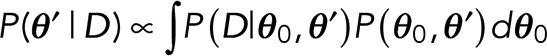 (3) (3)
|
For discrete parameters, the integral is understood as a sum. The marginal posterior now only depends on the remaining parameters, θ ′, that we want to determine and thus not integrate over.
The marginal posterior obtained from Eq. 3 is our starting point. Our goal is to find the model that maximizes this marginal posterior, where the likelihood appearing in Eq. 3 is given by Eq. 1 and the prior, which we now describe in more detail, depends on the parameters θ = (s, K, m, arr, μ, σ, γ ).
Here s are the event locations, K is the number of steps (i.e., discrete jumps in the data), m is the total number of events (defined as single-fluorophore intensity changes; from now on, when we refer to events, we exclusively mean these single-fluorophore intensity changes), arr is the number of possible arrangements of single-level events m (which we later ascribe to fluorescence intensity changes of magnitude μ = μf) on K steps (Figure 3), μ and σ are the mean and SD, respectively, and γ is a hyperparameter discussed in the Appendix.
FIGURE 3:

Two models can have the same number of steps and even have those steps occur at identical locations, and yet different m’s and arr’s may fit the data very differently. (A) m refers to the total number of single fluorophore intensity level changes. In both cases, K = 3 (three steps), but on the left, these are made up of a single, a double, and again a single event for a total m = 4, whereas on the right, the three steps are made up of a triple, a double, and a single event, and so m = 6. (B) arr refers to the different ways in which m events can be arranged in K steps. In both cases, K = 4 and m = 7 but arr is different. On the left, the first three steps are double-event ones and the fourth is single, whereas on the right, we have in succession a triple, a double, and two single events. Note that neither m nor arr is location dependent.
Taking all of the above into consideration, we write the prior as
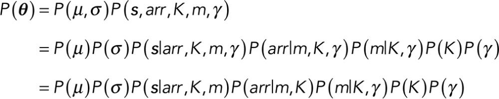 (4) (4)
|
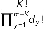
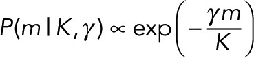
In writing Eq. 4, we assumed that μ and σ are independent. We also dropped the hyperparameter, γ, dependence from all conditionals except P(m|K, γ ) because γ couples only m to K. The factor P(s|arr, K, m) in Eq. 4 refers to the locations of the steps given the arrangements, number of steps, and number of events. Because we have no prior expectation on how step locations are affected by arr, K, and m, we always assume a flat (constant) prior P(s|arr, K, m). The form of the remaining prior terms depends on the conditions of our problem, which we motivate in the next two subsections.
Illustrative example: a model selection criterion assuming no event blinking or overlap.
Here, as an illustrative example, we derive a simpler model selection criterion using the steps highlighted earlier in the absence of blinking and overlap. Although this will not be useful in finding the model for a real photobleaching trace in which these complications are present, it serves a pedagogical purpose by illustrating how we reach a marginal posterior starting from a likelihood and set of assumptions that are built into a prior. More explicitly, our assumptions for this subsection are as follows. 1) Events do not overlap with each other (i.e., no two fluorophores photobleach at the same time, i.e., within the same data acquisition interval; Ulbrich and Isacoff, 2007). Simultaneous photobleaching is of particular concern for high fluorophore numbers and, as a consequence of the stochasticity of photobleaching and the finite sampling rate of instrumentation, cannot in practice be completely avoided. 2) Blinking (Annibale et al., 2011), due to either triplet states or long-lived dark states (Ha and Tinnefeld, 2012) arising from fluorophore conformational changes or interactions with the environment—where a fluorophore turns off reversibly and then reactivates—does not arise. In other words, at t = 0, all fluorophores are in the active state and, subsequently, may only irreversibly photobleach.
Because we have no blinking or overlapping events, the total number of events, m, in the trace is equal to the number of steps, K, and also equal to the total number of identical fluorophores, I, in an ROI, which is also the total number of states. The quantity arr has no meaning here and need not be considered (only one arrangement with one event per step is possible).
For this simple example, the likelihood of the model is
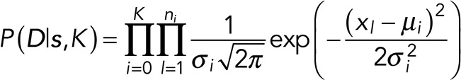 (5) (5)
|
Next, for our prior given by Eq. 4, because m = K and the quantity arr has no meaning, we set the prior terms as follows: P(arr|m, K) and P(K) to constants; P(m|K, γ ) ∝ δ(m−K), and, thus, P(γ ) to a constant.
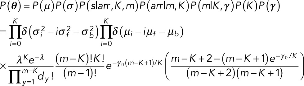
In our prior, however, we do assume that the photophysics of our problem properly informs μ and σ. That is, we assume that, in our prior, P(μ) = ΠIi = 0 P(μi) = ΠIi = 0 δ(μi − iμf −μb) and P(σ) = ΠIi = 0 P(σi) = ΠIi = 0 δ(σi2 − iσf2 − σb2). We then insert this likelihood and prior into our expression for our marginal posterior, Eq. 3, and subsequently marginalize the resulting posterior over all quantities except those that we want to use to discriminate between models, namely {s, K}. The resulting marginal posterior is simply
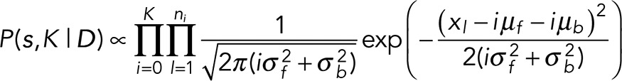 (6) (6)
|
where s are the step locations, a subset of K (out of a total N) data points. Of course, the particular data points that are members of the step location set change between models to be compared. Taking the negative log and dropping all constant terms, that is, terms that do not depend on model parameters, we get
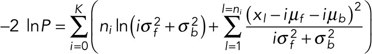 (7) (7)
|
Because the photophysics informs both our means and SDs, this expression differs from simple cases in which we integrate over all possible values of μ for every step and assume a single σ over all steps over which we also integrate, yielding
|
|
where N is the number of data points in the trace and  is defined in Eq. 3 of the Appendix of Kalafut and Visscher (2008).
Typically, if a fit to the data is bad, the likelihood function and, by extension, the marginal posterior are small. However, if we were to overestimate the number of active fluorophores at some point in the time trace, the expected variance would also grow (if we assume that both means and variances grow with i, as we did in Eq. 7). As uncertainty grows, poor fits to the data do not penalize the likelihood function as heavily as if the SD were small.
Concretely, what this means is that if we introduce the possibility of overlapping events, then our marginal posterior, as shown in Eq. 7, will 1) tend to overestimate the number of active fluorophores and 2) be consistently biased toward maximizing event overlap.
To address these problems, we need to incorporate the appropriate combinatorial factors that will inform the prior on how improbable it is for events to overlap. For example, we should be able to quantify, given no data, what the a priori odds are that the only two steps in a time trace containing 100 data points, say, overlap.
The next section treats blinking and overlap and deals with this key issue.
A criterion that incorporates blinking and overlapping events.
The following conditions hold when we have blinking and overlapping events in a photobleaching time trace:
States are no longer visited sequentially. For example, it is possible to go from state i to state i − 1 and then, say, back to state i.
Some states may be visited more than once (when blinking occurs).
Some states may not be visited at all. For example, if overlapping photobleaching events force the system to go directly from having i + 1 to having i − 1 active fluorophores without ever visiting state i.
Under these conditions, our likelihood is given by Eq. 1. Our full prior is given in Eq. 4. We assume the same priors over μ and σ assumed in the last subsection.
However, to correct for the bias we mentioned in the previous section on overlapping events, we introduce a combinatorial prior on P(arr|m, K):
 (9) (9)
|
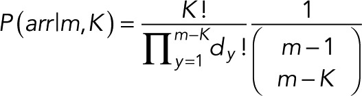
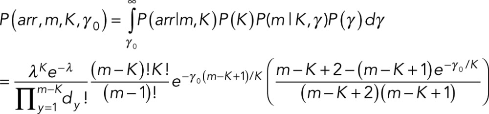
where m − K is the maximum number of events that can overlap, and dy are the degeneracies of steps with y-level “occupancy.” Further details are in the Appendix. Intuitively, this quantifies how unlikely it is to have many steps with multiple overlapping events. In addition, we specify priors on P(K), P(m|K, γ), and P(γ) as follows:
 (10) (10)
|
Here the prior over K is a Poisson distribution, which depends on the hyperparameter λ, the rate. In theory, our a priori assumption should have been that we have an inhomogeneous Poisson process with a higher rate expected at the start of the time trace (when many fluorophores are a priori expected to be active) and a lower rate expected at the end of time trace (when many fluorophores are a priori expected to have photobleached). Under these assumptions, we can estimate the precise form of λ and how it depends on another hyperparameter (the number of a priori expected active fluorophores at the start of the trace). In practice, in data analysis, an average—fixed value—for λ suffices.
Next our prior over γ penalizes deviations of m away from K. Because the strength of the penalty γ is unknown, we integrate this hyperparameter starting from some minimal acceptable value γ 0 to infinity. Further details are provided in the Appendix. As a final note, because we set λ to a fixed value that we do not integrate over in our prior over K, for notational simplicity, we do not introduce a prior over λ.
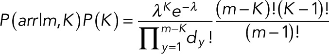
Inserting our priors for μ and σ and Eqs. 9 and 10 into Eq. 4 returns our full prior.
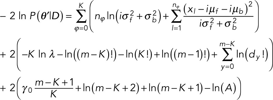
Next, inserting this full prior and the likelihood into Eq. 3 and following the appropriate marginalization over γ detailed in the Appendix and all integrations over δ-functions, we recover our marginal posterior:
 (11) (11)
|
where we dropped all constants that do not depend on model variables and defined 
Equation 11 is the criterion we use in model selection. As a simple sanity check, we note that Eq. 11 reduces to Eq. 7 when m = K with the exception of the single term –K ln λ, which arises out of the prior for P(K), which we had taken as constant in deriving Eq. 7.
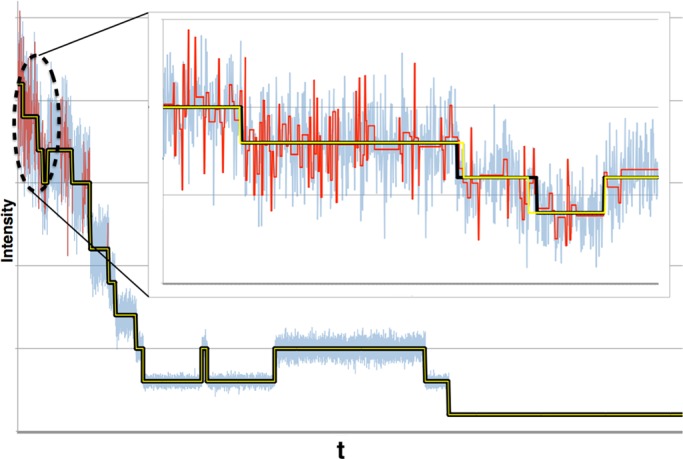
An example illustrating the key role of the prior is shown in Figure 4. In Figure 4A, we first show a model that maximizes the marginal posterior but does not consider blinking or overlapping events and further integrates over all values of μ and σ as was done in Eq. 8. In Figure 4B, we show that the model maximizing the marginal posterior that accounts for the photophysics in μ and σ via the appropriate prior but otherwise ignores blinking or overlapping events, Eq. 7, has two problems: 1) it overestimates the number of active fluorophores, and 2) it stacks events. Both problems arise for the reason we describe at the end of Illustrative example: a model selection criterion assuming no event blinking or overlap. In Figure 4C, we add explicit priors over P(K) and P(arr|m, K), which improve the model fit to the data primarily by reducing the number of events stacked. However, the number of active fluorophores is still overestimated without a prior on P(m|K, γ). Finally, in Figure 4D, we show that the model criterion given by Eq. 11 improves the fit for these low-noise data.
FIGURE 4:

Our method’s accuracy increases as more prior terms are specified explicitly. We used low-noise experimental data from the Peterman and Wuite groups to test the effects of our prior. (A) No blinking or overlapping events are considered, and we integrate over all unknown means and variance to obtain the marginal posterior. Although some steps are found accurately, others are not, and both the double-step and the reactivation events are predictably missed. (B) Here we use the marginal posterior given in Eq. 7, which, as expected, shows event stacking and overestimation of the number of active fluorophores for the reasons described in Illustrative example: a model selection criterion assuming no event blinking or overlap. (C) Here we add the explicit form of the priors for P(K) and P(arr|m, K). The overestimation of fluorophore numbers problem is resolved, although the algorithm still gets the event stacking wrong, causing a step to be missed. (D) Our full posterior, Eq. 11. Results are excellent compared with A–C.
Algorithm description
In practice, computing and comparing the marginal posterior, or equivalently Eq. 11, for all conceivable models is not computationally feasible. To reduce the computational cost, nested (also called greedy) approaches are used (Chen et al., 2014), in which, for instance, a single trial step is placed at a point in time and a selection criterion, such as the SIC or AIC, is calculated. If a single step provides a value for the criterion that is lower than the criterion with no step, then this step is retained, and the process is repeated (holding the first step fixed) to find the possible location of a second step. More steps are subsequently found in this way until any single additional step only increases the value of the criterion. Although this approximate treatment is relatively efficient, it still requires roughly O(NK) calculations, where N is the total number of data points and K, as before, is the total number of steps.
Instead of this classic nested approach, to improve computational efficiency and accuracy (defined later), we employ the following three-step method.
Step 1: We find the mean and SD of the single fluorophore and background from the data, if not already known experimentally. In other words, assuming μf, σf, μb, and σb are a priori unknown, we determine these quantities by employing a version of a greedy algorithm (Kalafut and Visscher, 2008) to locate the last steps in the trace—that is, where the noise level is lowest —that provide us with an estimate for μf, σf, μb, and σb.
Step 2: Eliminate unlikely models. We propose a principled method to eliminate a vast number of improbable models (e.g., such as the extreme example of having all fluorophores simultaneously photobleach), leaving our criterion, Eq. 11, to evaluate the relative merit of a comparatively smaller number of candidate models. To do so, we first subdivide our time trace into G windows of nc data points each. The first window is defined as the window at the very end of the time trace. Now, knowing μf, σf, μb, and σb from Step 1, we have an estimate for how many fluorophores are active in the first window. As we begin moving in reverse time order—eventually toward the start of the trace (Gth window)—we may estimate how many fluorophores must be active in each window.
To estimate the fluorophore number in each window, we note that any data point along a photobleaching time trace must ultimately be sampled from a normal probability distribution, pi, of mean iμf + μb and variance iσf2 + σb2. For each sequence of nc data points, we can quantify the likelihood that all nc data points were sampled from pi. This is the likelihood that all points in that window were sampled during a time when i fluorophores were active, given the data in the window. The most likely number of fluorophores active in each window is the specific value of i for which this likelihood is maximum.
We assume that in the first window (which is the last timewise, since we are moving through the data in reverse), all data points are sampled from p0. We then move to the next window, where we compare the values of the likelihoods for a certain range of i values based on the number of fluorophores that were active in the previous window we examined. For example, if in the previous window the most likely number of active fluorophores was k (so that the data were drawn from pk), we search the distributions {pk−imax, pk+1−imax,…, pk−1+imax, pk+imax}, where imax is set to some arbitrary but reasonable value depending on k. If k − imax < 0, we stop searching at p0 since there can never be a negative number of active fluorophores.
Any time two neighboring windows are found to have different numbers of most likely active fluorophores, say pα and pβ , where we take α > β, then α − β events have probably occurred. Moving in reverse through the trace in this manner, we estimate the most likely number of events that occurred in any window (Figure 5). Note that dividing up the data set into small windows increases both accuracy and computational time. However, very small windows introduce error due to small number statistics and should be avoided.
FIGURE 5:
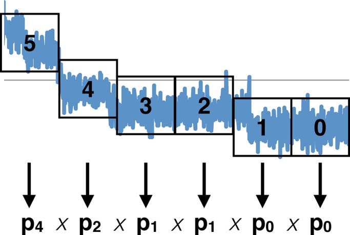
How Step 2 of our algorithm works: The synthetic data (blue) are divided into G = 6 windows (black squares). For each window, we calculate i likelihoods. Each of these is the likelihood that all data points within the window were taken when i fluorophores were active. Once we have all i likelihoods, we compare them and assign the window the number of fluorophores for which the likelihood is maximized. In this example, Step 2 has determined that the data points in windows 0 and 1 most likely belong to the p0 distribution (no fluorophores active, only background), the data points in windows 2 and 3 most likely belong to the p1 distribution (one fluorophore active), and the data points in windows 4 and 5 most likely belong to the p2 and p4 distributions, respectively, which means that two fluorophores are active in window 4 and four in 5. When Step 3 of our algorithm treats this trace, it will use the results from Step 2 to focus on reasonable preselected models. For example, it will focus primarily on models that have two to four active fluorophores in windows 4 and 5.
Step 3: Precisely determine step location and numbers. We now use the information from Step 2 to determine the most likely event locations. Scanning in reverse the window segmented data, we compute the numerical value of Eq. 11 for all possible event locations within a window, knowing, from the previous step, that the most likely number of events occurring within the window is α − β. Assuming some error in our Step 2 estimate of α − β events, we compute the value for all possible events in the range [(α − β) − w, (α − β ) + w]. If the value of Eq. 11 at one of the limits of the search range (say, (α − β) + w ) proves to be the smallest, we recenter our search on that value and calculate values for our criterion with ±w again (continuing the example, in [(α − β ), (α − β ) + 2w]). Comparing these values, we assign the one with the minimum value as the most probable local model. Like imax and nc, the range of events to be considered, w, is set by the user on the basis of computational efficiency. Benchmarking on synthetic data reveals that small w’s decrease accuracy and computational cost, whereas large ones do the reverse. Note that w and imax are the same concept, in that both designate the range of our search for the most likely number of active fluorophores, doing so in Steps 1 and 2, respectively. However, we denote them differently because the much heavier computational demands of Step 3 necessitate that w be much smaller than imax. Simply put, Step 2 is so much simpler computationally that imax can easily be in the hundreds, whereas a w >10 or 20 becomes computationally prohibitive.
To summarize, after determining μf, σf, μb, and σb in Step 1, in Step 2, all windows are scanned in reverse order, and an estimate of the number of steps in each window is made. We then move to Step 3 and calculate the most likely model. A schematic of our algorithm appears in Figure 6. For a total number of G windows of size nc with α − β events per window, we must compute the criterion value a number of times that is roughly of the order Gnc(α − β ). If we set N = 100,000, I = 50, G = 1000, nc = 100, and α − β = 5, we get that a nested algorithm requires NI = 5 × 10⁶ calculations, whereas our method requires Gnc(α − β ) = 5 × 10⁵ calculations. In other words, our approach reduces computational requirements by an order of magnitude. In reality, because photobleaching is an exponential process, the vast majority of windows especially toward the end of the trace will have few or no events. Therefore Step 3 will either not need to be used or will have to discriminate between very few candidate models for those windows, so our approach is even faster than this upper bound. For typical photobleaching time traces with up to 103 data points, our algorithm works in seconds. For data sets that have between 1000 and 10,000 data points our algorithm runs in seconds to a few minutes. For very large data sets, our algorithm works faster than other methods we have tested. For example, in a test of a very large data set that was specifically designed to be hard to fit, performed on an ordinary MacBook Pro 2.5 GHz laptop, the Tdetector2 algorithm, which is based on Student’s two-sample t test as implemented in MATLAB by Chen et al. (2014), required ∼7 d to run the 5 × 10⁴–data point data set with 50 steps; our method needed 17 h.
FIGURE 6:

The three steps of our algorithm can be broken down into a step-by-step chart. In this schematic, nc is the window size, imax is the maximum number of fluorophores simultaneously considered in a window, w is the maximum number of single-level fluorescence change events the code will consider (essentially setting m = w, but only within one window), and γ 0 is a hyperparameter cutoff. These four quantities are the user-defined parameters that our approach requires. Note that since the trace has been reversed, the “first” window and the “first” two steps of the algorithm discussed in Kalafut and Visscher (2008) are timewise the last window and the latest two steps in the trace.
Applicability of our approach: theoretical and computational limitations
There are two major constraints to our method’s applicability:
We assume that each individual fluorophore is independent and has identical properties μf and σf that do not change in time. This assumes that the fluorophore maturation process is complete for all fluorophores; that, following a blinking event, the fluorophore fluoresces just as it did earlier; that all fluorophores are imaged on nearby z-planes; and that the orientation of fluorophores that are not freely rotating does not affect their fluorescence properties (Backlund et al., 2014). For example, for a large complex, one can imagine that the observed fluorescence intensity of a particular fluorophore within that complex might depend on the fluorophore’s orientation and location within the complex, so that not all photobleaching events give rise to an equal μf (Backlund et al., 2014), or, if a fluorophore is not freely rotating, the number of detected photons emitted by the fluorophore might depend on the angle between their orientation and the detector, which could change over time. We might deal with this challenge by ascribing a prior over the μf’s informed by the physics of the problem and integrating over a range of acceptable μf’s in our posterior.
Our method is only as good as the data. With insufficient data, step locations can no longer be reliably determined. Thus we assume that the data resolution is high enough that even at the start of the trace, the number of data points between fluorescence level changes is at least 50. This number of data points between steps is sufficient for adjusted SNR (aSNR), where aSNR = 2(μϕ +1 − μϕ)/(σϕ +1 + σϕ), and ϕ is an interval (for the full definition of aSNR, see Results) down to 0.25. If the aSNR is larger, we need fewer data points between steps to be accurate. On the contrary, if the aSNR is smaller, we need larger numbers of data points between steps for our algorithm to accurately locate them. Having few data points between events runs the risk of introducing small-number statistics errors in our method, primarily in the form of having close-by real steps confused for double steps. However, it is often the case that, even when the aSNR is low (<0.25) and the data points between steps <50, our algorithm yields correct results. Still, if both aSNR and number of data points between steps decrease, confidence in our algorithm’s results should decrease as well. For most systems, the number of data points acquired between possible steps is a matter of experimental design. Whereas fluorophore photobleaching is a random process and events with separation <50 data points are bound to occur, by tuning, for instance, laser intensity, an experiment can be designed to ensure that the majority of events have a separation of >50 data points on average.
RESULTS
Benchmarking on synthetic data
To test our algorithm’s performance, we first test our method on synthetic data sets in which the actual step locations are known. We start by discussing qualitative comparisons and subsequently define metrics that will allow us to make quantitative comparisons.
All data sets were created using the Gillespie algorithm (Gillespie, 1977) by starting with N fluorophores each with prespecified kinetics (photobleaching and blinking-on/off rates). We then created a trace, which we call the noiseless or denoised time trace, by plotting the total number of active fluorophores multiplied by μf and then added noise.
Once we generated these data, we ask whether we can determine the number of steps, K, and their locations, s. We tested various choices of hyperparameters and user-input parameters (n, imax, w, etc., as defined in our algorithm) for the best results as quantified by the metrics defined later. To measure our algorithm’s performance and compare it to alternate tools, we tested various methods (including our own) on our synthetic data sets.
The performance metrics we use are based on the number and location of events—which, we recall, are single-fluorophore intensity level changes—because a step may be made up of more than one single event when considering overlapping events. Our metrics are defined as follows:
Precision (PR): the ratio of the number of true events found (exact or displaced; see later discussion) to the total number of events found.
Sensitivity (SE): the ratio of the number of true events found (exact or displaced) to the total number of true events.
Offset (OF): the average distance (in terms of data points) between the location of a true event and the location of the found event. This is a metric that can capture the cases in which an event is identified close to, but not quite on, its true location, in which case we call it a displaced true event.
We identify an event as a displaced true event only if the event found is within a distance d (in terms of data points) from the true event. We set d to be the minimum of 50 data points or 0.1%N, where N is the total number of data points in an entire trace. If more than one event is found within d of the true event, we take the closest one as the displaced event. If both are equally distant from the true event, we conservatively accept neither as a displaced event and consider the true event as missed. If a step found is not of size (number of single-level events) equal to the corresponding true step, we only consider correct the number of events up to overlap size. For example, if there is a triple step in the trace but we only find a double step, we consider two events found and one event missed. Similarly, if there is, say, a reactivation event and we find a double step, we consider three events missed.
4. Adjusted signal-to-noise ratio (aSNR): defined as 2(μϕ + 1 − μϕ)/(σϕ + 1 + σϕ), where μϕ and σϕ are the mean and SD of the ϕ th interval (recall that an interval is the stretch of data points between two identified steps). This is a step-specific measure of the noise that, contrary to the simpler μf/σf metric, captures the increasing difficulty of identifying a step when there are many active fluorophores (i.e., at the start of a trace). aSNR is given as a range from its value at the trace end to its value at the trace start.
Under these metrics, optimal performance implies unity precision and sensitivity (all true events found and no false events found) and zero offset (all events found at their precise locations), whereas the range of aSNR is a measure of how hard a data set is to fit. These metrics can be used to compare algorithm performance on synthetic data sets but cannot be used on real experimental data, where the true steps are unknown.
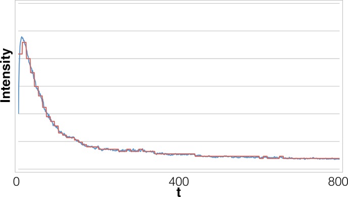
Figure 7A shows the example of a time trace with many fluorophores initially active (the black line is the theoretical noiseless trace). Figure 7B shows the data from Figure 7A with the results from Step 2 of our algorithm offset in red and the results of our full algorithm offset in blue. Both blue and red show a spurious blinking event at the start of the trace, where the noise level is highest. Otherwise, blue matches the ground truth (black) almost exactly, whereas red is only an approximation. This shows how Step 2 of our algorithm successfully approximates the real denoised model, thus greatly reducing the number of alternate models our Step 3 needs to consider. The net effect of producing a good approximation such as this is that computational resources and time are substantially reduced. In Figure 7C, we overlap the ground truth (black) with the results (green) from our full algorithm to further illustrate how precise our results are.
FIGURE 7:

Example of our method applied to a data set with high numbers of fluorophores and correspondingly high noise levels. (A) Large numbers of fluorophores produce a very noisy trace (synthetic data). This is an example of a noisy signal (blue) around the denoised trace (black) for synthetic data. We show the first 104 data points from a 2 × 10⁵ data point trace in which 50 fluorophores photobleached. For this data set, μf = 2.0, σf = 0.2, μb = 20.0, and σb = 0.0. (B) Step 2 provides a rough estimate of the ground truth trace that Step 3 refines. We show the same denoised levels and noisy data as in A plus the estimate from Step 2 (red; after eliminating unlikely models) and Step 3 (blue). The red and blue curves have been displaced by −20 and +20 intensity points, respectively, to facilitate comparison. (C) The same denoised levels (black) and noisy data (blue) from A, where we superimposed the results of our approach after Step 3 (green), Eq. 11, on the denoised data levels to emphasize differences. We find all steps with (in some cases) minor offsets only, so our sensitivity is optimal (SE = 1), and offset is very good (OF = 0.84). At very high fluorophore numbers, our algorithm detects one spurious blinking event, but that is the only error, and so that precision is near perfect (PR = 0.99). aSNR = 10–0.2.
Analysis of the experimental data sets
We present the analysis on five data sets:
Data set I (published data): We used green fluorescent protein (GFP)–tagged mitotic centromere–associated kinase (MCAK) protein provided by the Walczak group (Ems-McClung et al., 2013). MCAK proteins—members of the kinesin-13 protein family—are involved in spindle assembly during mitosis, chromosome segregation, and error correction (Walczak et al., 2013). MCAK is also unique among kinesins because it can bind to microtubule ends directly from solution and rapidly diffuse along the microtubule; once attached to the microtubule’s end, it causes a conformational change that results in microtubule depolymerization and its own detachment. It is known (Walczak et al., 2013) that when Aurora B kinase phosphorylates MCAK, the latter’s depolymerization activity is inhibited. To discover the mechanism of inhibition, MCAK proteins were tagged with GFP, and photobleaching event counting was used to see how quickly they detached from a microtubule.
Data set II (published data): We used Alexa Fluor 55–tagged RAD51 proteins provided by the Peterman and Wuite groups (van Mameren et al., 2009). RAD51 is a recombinase protein. It catalyzes strand exchange between homologous DNA segments (Sung et al., 2003), a key meiotic event that assures genetic diversity (van Mameren et al., 2009). RAD51 forms a helical filament around single-stranded DNA; this filament then locates the homologous double-stranded DNA, invades it, and catalyzes the strand exchange needed to create a joint molecule, following which the RAD51 filament disassembles to enable other proteins to conclude the process. The disassembly from the filament requires hydrolysis of ATP bound at the interface between adjacent RAD51 monomers. To determine the precise disassembly mechanism, RAD51 monomers were labeled with Alexa Fluor 555 and photobleaching time traces taken to determine the number of monomers per filament and their detachment rate from the filament.
Data sets III–V (new data): Here we used our method on data sets acquired during experiments intended to investigate how drug delivery systems (DDS) work at the cellular level. A challenge in the optimization of DDS is the ability to accurately quantify when, where, and how much drug release occurs inside the targeted cell. Recently ensemble fluorescence microscopy–based techniques have begun to be used to simultaneously answer these questions in a semiquantitative manner. Although these experiments sufficiently guide scientists to determine when large release events occur from endosomal compartments, they are insufficient to analyze slow-release events, low DDS concentrations, and events that occur outside of the endocytotic transport pathway (e.g., directly into the cytoplasm). By contrast, photobleaching event counting holds the promise to quantify release of DDS cargo more accurately (Pitchiaya et al., 2012, 2013, 2014; Shankar et al., 2016).
Data set analysis results
Having benchmarked our method on synthetic data, we now summarize our method’s analysis of all experimental data sets in Figures 8–12. For data set I (Figure 8), our algorithm identifies four fluorescence levels (including the background-only level). For data set II (Figure 9), our method finds two steps and determines that the very first data points in the trace arise from noise and not a third fluorophore. Considering that both traces have high SNR (∼2 and ∼4, respectively), we can verify our algorithm’s findings by eye.
FIGURE 8:
Our analysis of a trace obtained on GFP-tagged MCAK protein. These data are expected to show a large reactivation event and two or three steps, as the GFP-tagged proteins that have attached to a microtubule are first activated and then detach from the microtubule. Our method identifies the initial triple activation (a large initial activation event is expected when the fluorophores are first illuminated) and then finds two more steps (one double and one single). Given the small number of fluorophores and the low noise level, our findings are consistent with steps identifiable by eye.
FIGURE 9:

Our analysis of a trace obtained on Alexa Fluor 555–tagged RAD51 proteins. In keeping with our expectation for how noise should change as more fluorophores are active, we identify two steps and determine that the small rise at the very start of the trace arises from noise, contrary to the analysis in van Mameren et al. (2009). At low noise, our findings are again consistent with steps identifiable by eye.
FIGURE 10:
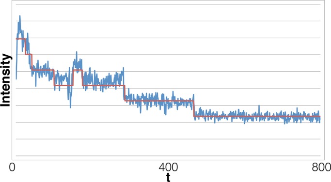
Our analysis of a trace obtained from HeLa cells transfected with Alexa Fluor 647–tagged microRNA-7. Our method locates seven steps in this data set, including two steps ascribed to blinking-on/off events. By contrast, the original analysis method found only three steps. The difference may be due to the fact that the original analysis method used filtering and averaging, which smooths out features of short duration, such as blinking.
FIGURE 11:
Our analysis of a trace obtained from HeLa cells transfected with Alexa Fluor 647–tagged microRNA-7 with drift. Our method marks four steps in this data set, in agreement with the original analysis method, despite the fact that early in the data set, the intervals between steps have <20 data points, making our method susceptible to error due to small-number statistics. Also note that this trace exhibits a slow, gradual decline in fluorescence that we believe is due to background autofluorescent endogenous material (Monici, 2005) colocalized with our fluorescent microRNA. These background particles typically photobleach slowly and show very small step sizes, leading to the visualization of a slow, steady decrease in fluorescent signal and making step detection difficult by eye. Our algorithm, which relies on specific anticipated noise changes for photobleaching event, does not misinterpret drift as photobleaching events, as can be seen toward the end of the time trace. In principle, however, in order to become more robust to drift, our likelihood function would need to incorporate those effects.
FIGURE 12:
Long time trace also obtained from HeLa cells transfected with Alexa Fluor 647–tagged microRNA-7. Our method marks ∼30 steps in this data set. The original analysis method found this data set intractable even after filtering. Our method finds not only many steps but also multiple blinking and overlapping events. Photobleaching events that are very close in time register as overlapping events if the data acquisition rate is longer than the interval between successive photobleachings.
For data sets III in Figure 10 and IV in Figure 11, our method’s results respectively conflict and agree with the results of the original analysis method, which was a combination of noise filtering and estimation of fluorescence levels identifiable by eye (a fuller description of the original analysis method can be found in later subsections on Trace extraction and Data analysis). Whereas this original analysis method concluded that there are three steps in Figure 10, our method finds seven steps because it identified a blinking event. On the contrary, for Figure 11, our and the original analysis method agree on four steps. We note that errors due to small-number statistics when processing data set IV are more likely than when processing data set III. We therefore have more confidence in our analysis of data set III, despite the fact that our method’s results disagree with the original data analysis method. For data set V in Figure 12, our method finds >30 steps, including multiple reactivation and overlapping events. The latter are particularly prevalent early in the trace, which is expected if there are many fluorophores active to begin with and the data acquisition rate is relatively low. This is because photobleaching events are more frequent early in a trace, and if more than one event occurs between successive measurements, they will register as an overlapping event. It is worth noting that the original filtering-and-eye analysis method found this data set intractable and could not resolve any steps.
Comparison to other methods
Our method treats blinking, stochastic noise variations, and overlapping events that may arise from interacting fluorophores or slower time acquisition. Our method can be generalized to treat a range of μf’s and σf’s, although in this work, we assume these are fixed to some determinable value.
In this section, we compare our approach to existing methods.
The first approach is based on hidden Markov models (HMMs; Messina et al., 2006). These methods are generally very reliable and have been used to great effect in other problems; however, for photobleaching event counting, HMMs are hampered because their computational cost quickly becomes prohibitive unless one limits the number of fluorescence intensity states that can be considered. For example, in Messina et al. (2006), working on multichromophore photobleaching, to make the model computationally tractable, it was necessary to postulate that only single-level jumps occur, thus eliminating the possibility to treat overlapping events; even so, the method is limited to counting 30–40 fluorophores.
Another common approach relies on using some test or criterion to determine the number and location of photobleaching steps. Such methods include the KV algorithm (Kalafut and Visscher, 2008), which assumes fixed noise and is captured by Eq. 8 and Student’s two-sample t test (Chen et al., 2014).
Chen et al. (2014) tested four different algorithms—two based on the SIC (with constant and variable variance) and two based on the two-sample t-tests—and concluded that the second of the two-sample t-test–based algorithms (called Tdetector2) was the best for photobleaching event counting. We compared our method to both the fixed-noise model, Eq. 8, and the Tdetector2 algorithm (Figures 13 and 14). We tabulate the comparison results in Table 2. Our method performs better than the fixed-noise model because it avoids the excessive overfitting exhibited by the fixed-noise model at the high-noise, high-fluorophore start of the trace. We also outperform the Tdetector2 algorithm because 1) it does not explicitly consider blinking and overlapping events, and 2) it overestimates the number of active fluorophores, a problem that we also encountered but resolved through our prior, which is discussed in more detail in the Appendix. We also note that the data set we used to test our algorithm against the Tdetector2 algorithm purposefully violates our desideratum of minimally having 50 data points between successive steps. Nevertheless, our algorithm still outperforms the alternatives; see legends to Figures 13 and 14 for details. As a final note, we stress that our algorithm does not involve smoothing or filtering, which removes information on fast–time scale kinetics.
FIGURE 13:
Our method greatly improves on the results of methods that treat noise as fixed. To compare the performance of Eq. 8 to Eq. 11, we use a 20,000-data point set of just 10 fluorophores (μf = 2.0 and σf = 0.2) photobleaching to background with aSNR = 10.0–1.0. We show the theoretical signal (thick black line) around which we added noise (light blue), our estimate (yellow line), and the result of Eq. 8 (red line). At the end of the trace, both methods do very well. However, at the start of the trace, where cumulative noise is highest, our method has only minor offset (OF = 2.4), whereas a fixed-noise model grossly overfits, finding >100 spurious steps. This is expected because the higher noise at the start of the trace is now interpreted as signal by algorithms that assume that noise is fixed. Note that both methods find all true steps (SE = 1 for both), but the overfit by the fixed-noise model leads to great disparity for precision (PR = 1 for our approach; PR ≈ 0.125 for Eq. 8). Inset, detail of the trace’s first 1000 data points, where the bulk of overfitting by the fixed-noise model occurs.
FIGURE 14:

Our algorithm offers an improvement over a recent Tdetector2 algorithm (Chen et al., 2014). In this 10,000–data point data set, 50 fluorophores photobleach to background with μf = 2.0, σf = 0.2, μb = 20.0, and σb = 0.0001. As before, we show the theoretical signal (thick black line) around which we added noise (light blue), the results of the Tdetector2 algorithm (red), and results of our approach (dark blue). The dark blue and red curves are displaced by ±15 fluorescence units, respectively, to facilitate comparison. Both algorithms do very well late in the trace, when noise is relatively low; however, as noise increases, both encounter problems. In particular, both algorithms underfit. For our method, such underfitting is expected due to small-number statistics (see later discussion). However, the Tdetector2 algorithm performs considerably worse. Inset, detail of the first 1000 data points of the trace. Underfitting for both algorithms is obvious, as is the fact that the Tdetector2 algorithm performs significantly worse than ours. We have aSNR = 10–0.1, PRB = 0.92, PRT = 0.81, SEB = 0.34, SET = 0.31, OFB = 22.0, and OFT = 39.1, where the subscripts B and T denote our Bayesian method and the Tdetector2 algorithm results, respectively. Note that this particular synthetic data set was purposefully constructed to be “hard” for our algorithm to process: there are numerous cases in which neighboring fluorescence change events are separated by <50 data points. For aSNR ≤ 0.25, 50 points is the minimum number of data points between steps that permits our algorithm to perform relatively reliably. If the number of data points between steps is smaller, small-number statistics introduces error into our algorithm.
TABLE 2:
Comparison of photobleaching event counting algorithms.
| Parameter | Constant noise method | Tdetector2 | Our method |
| Precision | 0.1 | 0.73 | 0.95 |
| Sensitivity | 1 | 0.47 | 0.82 |
| Offset | 1.2 | 45.6 | 13.7 |
Finally, there are many miscellaneous methods, from simple ones such as measuring the fluorescence “step” size from the late trace where steps can be detected by eye and using it to determine the number of fluorophores initially active, to more elaborate ones, such as using a Γ-distribution and dividing starting intensity by the result (Coffman and Wu, 2012), to using a binomial distribution with many traces to determine the most probable maximum fluorophore number (Das et al., 2007), to using the propagation of information with feedback algorithm (McGuire et al., 2012). Such methods have faced problems when dealing with a large number (20–30) of fluorophores and low SNR.
A recent method, spot number intensity correlation (SONIC; Liesche et al., 2015), is an innovative method that determines the total number of fluorophore-tagged subunits based on a statistical analysis of measurements of the time to total bleaching of all fluorophores in a complex. Because complexes with more fluorophore-tagged subunits take longer to decay to background fluorescence, the statistical analysis can yield an estimate for the total fluorophore number without determining exact step locations. SONIC seems to be very accurate when determining the number of fluorophores, but it has a major drawback, in that it cannot locate photobleaching steps in time and therefore cannot address problems for which kinetic measurements are needed, such as when MCAK proteins move in and out of the spindle assembly during mitosis.
Discussion
Superresolution single-molecule microscopy methods are poised to provide information on protein complex stoichiometry with high spatial resolution (Lee et al., 2012; Rollins et al., 2015). Spatial resolution in itself is important because it may distinguish, for instance, between true colocalization of protein species and random spatial patterning below the diffraction limit (Xia et al., 2013).
Despite its advantages, counting from superresolution data may become computationally expensive (Rollins et al., 2015) except when realized via very sparse activations—but in that case, the experiments are difficult—and may be complicated by photophysical artifacts such as incomplete maturation of the fluorophore (Durisic et al., 2014).
Although photobleaching event counting does not provide subdiffraction-limited information, it is computationally inexpensive and, for this reason, more complicated effects (such as blinking) can more feasibly be incorporated into the analysis of larger data sets. Here we argue that the key to successfully analyzing large photobleach data sets is to use the expected physics of the fluorophores to inform the step-finding process. This strategy reduces the number of errors arising from stochastically varying noise, blinking, and event overlap that arise in the methods to which we have compared ours.
For simple cases with few (<20) fluorophores or high aSNR (>1), our method does better than or just as well as coarser algorithms that ignore variance changes or blinking and overlap. However, our method does remarkably better on more challenging synthetic data sets and, presumably, would perform equally well in experimental data sets involving 50+ fluorophores, (Figure 7), as suggested by our analysis of data set IV provided in Figure 12. This should help motivate future, more challenging experiments in which the number of fluorophores is much higher and their photophysics may be more complex.
MATERIALS AND METHODS
Here we describe the experiments that produced the unpublished data sets that we tested with our method.
Preparation of fluorescent microRNA duplexes
MicroRNA-7 (miR-7) guide and passenger oligonucleotides were synthesized with a 5′ phosphate and, in the case of the labeled guide strand, a 3′ NHS-ester–linked Alexa Fluor 647 (Integrated DNA Technologies, Coralville, IA). Guide and passenger strands were HPLC purified by Integrated DNA Technologies, and their size and purity were verified by denaturing, 8 M urea, 20% PAGE. For the guide strand, 90% of the RNA was found to be singly labeled, as determined by quantifying the molar ratio of fluorophore to RNA through ultraviolet–visible absorbance measurements. Guide and passenger strands were heat annealed at a 1:1.5 ratio in 1× phosphate-buffered saline (PBS; 70011; Life Technologies, Delhi, India) to a final concentration of 10 μM. The extent of duplex formation was assessed using an electrophoretic mobility shift assay on a nondenaturing 20% polyacrylamide gel. The miR-7 passenger and guide strand sequences were as follows:
miR-7 guide: 5′-p-UGGAAGACUAGUGAUUUUGUUGU-3′,
miR-7 passenger: 5′-p-CAACAAAUCACAGUCUGCCAUA-3′.
Cell culture and transfection
HeLa cells (CCL–2; American Type Culture Collection, Manassas, VA) were grown in an incubator and held at 37°C in an atmosphere with 5% CO2 and 95% relative humidity. Cells were maintained in DMEM (11995; GIBCO, Langley, OK), supplemented with 10% (vol/vol) fetal bovine serum and 100 U/ml penicillin–streptomycin (15140122; ThermoFisher Scientific, Waltham, MA). On reaching ∼80% confluency, cells were split and seeded onto DeltaT (Bioptechs, Butler, PA) dishes to a density of 1 × 10⁵ cells/dish. After 24 h, each dish of cells had half of its medium removed and was supplemented with 500 μl of transfection mixture (Lipofectamine 2000 [11668019; Invitrogen, Carlsbad, CA] and 40 pmol of miR-7 duplex in OptiMEM [31985070; Invitrogen]). To prevent overloading the cell with excessive fluorescently labeled miR-7, only 1% of the total duplexed guide strand contained Alexa Fluor 647. After a 4-h incubation period, the transfection mixture was replaced with fresh medium. At 6 h after transfection, the cells were washed thrice with 1× PBS, followed by a 20-min incubation with a 4% (wt/vol) paraformaldehyde and 1× PBS mixture for fixation. The cells were then washed thrice with 1× PBS, immersed in oxygen scavenger system (OSS; 5 mM protocatechuic acid, protocatechuate-3,4-dioxygenase, and 2 mM Trolox [6-hydroxy-2,5,7,8-tetramethylchroman-2-carboxylic acid]), covered, and sealed using Valap sealant.
Single-molecule imaging
Microscopy imaging was conducted as previously described (Pitchiaya et al., 2012, 2014, 2013; Shankar et al., 2016), using a home-built IX-81 Olympus microscope with a 60×, 1.49 numerical aperture oil immersion objective (Olympus, Lombard, IL), 2× magnification wheel, P–545.3C7 capacitive piezoelectric xyz-stage (Physik Instrumente, Karlsruhe, Germany), iXon 897 (Andor, Belfast, United Kingdom) electron-multiplying charge-coupled device camera, and a Cell-TIRF module (Olympus). Cells were illuminated using solid-state lasers with wavelengths of 405 nm (0.8 mW at the objective) and 640 nm (8 mW at the objective). Highly inclined laminar optical sheet (HILO) microscopy was used to achieve sufficient illumination depth while minimizing background. A quadband dichroic (Chroma) 405/488/532/647 was used to detect miR-7 fluorescent particles and cell boundaries. All videos were acquired at a 100-ms camera exposure time for 400 or 600 frames.
Trace extraction
Original trace analysis (done and then compared with the method described here) was performed using a custom-written LabView (National Instruments, Austin, TX) software code similar to previously described procedures (Pitchiaya et al., 2012, 2013). In short, the LabView code uses noise-filtering and photon-counting histogram algorithms to identify particles of interest and removes nonuniform background from all selected traces. The data were filtered further by a nonlinear Chung–Kennedy noise filter to preserve fast and sudden signal transitions while averaging out random noise. The filtered data were then assessed by eye, with each sudden decrease in signal classified as a photobleaching event. For each trace, the number of photobleaching events corresponds to the total fluorescent miR-7 molecules within a focus since >90% of dye molecules are found to be fluorescent (Pitchiaya et al., 2012, 2013).
Data analysis: fixed-cell photobleaching analysis of transfected fluorescent miR-7 duplex
To test the photobleaching event counting method described here in a biological context, we conducted a single-molecule photobleaching analysis to test the oligomerization state of transfected fluorescent miR-7 duplex in fixed HeLa cells. Six hours after transfection, our cells were fixed in a 4% paraformaldehyde solution, immersed in OSS, and illuminated using HILO fluorescence microscopy. Videos of single cells were acquired until all cellular fluorescent particles were photobleached into a permanent dark state. The original analysis was performed as described; via our custom LabView software, fluorescent particles were identified and background subtracted. Then noise was filtered to help identify by eye intensity transitions relevant to the photobleaching process. The results of this original analysis method were then compared with the results we acquired by first using the Lab View code just to select areas of interest and then processing the traces with our full Bayesian code.
Appendix: explicit form of the priors over m, K, and arr and the prior we use to constrain m to K
Here we derive the explicit terms that go into the prior that informed our marginal posterior, Eq. 11, by detailing the form of the terms given in Eq. 4: P(arr|m, K), P(K), P(γ), and P(m|K, γ).
Explicit form of P(arr|m, K) and P(K): combinations with repetition
We start with two of the terms in Eq. 4: P(arr|m, K) and P(K). When determining how m events are distributed in a set number of K steps, we have, from the number of combinations of m with repetition on K sites, the following total number of arrangements:
 (12) (12)
|
The number of ways in which a particular arrangement of m’s can be realized is
 (13) (13)
|
where dy is the number of steps with single-level event “occupancy” y, and m − K is the maximum possible number of overlapping events. The normalized probability of a given arrangement is then
 (14) (14)
|
Next, to set a prior on the number of K within the time trace, we assume that, in the absence of blinking and overlap, the number of events is Poisson distributed for the reasons described in the text:
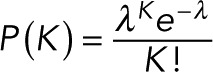 (15) (15)
|
Combining Eqs. 14 and 15, we obtain the prior over the number of steps K and the arrangements arr that arise for a given K and a total number of events m:
 (16) (16)
|
Recall that the likelihood has two problems: 1) it overestimates the number of active fluorophores and 2) it stacks events. It does so for the reasons spelled out in Illustrative example: a model selection criterion assuming no event blinking or overlap. The foregoing prior fixes problem 1. The next subsection fixes problem 2.
Priors over P(m|K, γ) and P(γ)
To constrain m close to K, which addresses problem 2 of the last subsection, we introduce the hyperparameter γ and write P(m, γ |K) = P(m|K, γ )P(γ ). We assign to P(m|K, γ ) an exponential form:
 (17) (17)
|
where we use a proportionality because we dropped the normalization obtained by summing the exponential of Eq. 17 over m from K to ∞ (recall that there can be no fewer events, m, than there are states, K). Because we are unsure about how strongly we want to enforce this prior assumption that m ∼ K, we integrate over γ (assuming flat P(γ)) from some minimal value γ0 to some upper bound that we set to ∞. Our prior is now
 (18) (18)
|
The full prior therefore becomes
 (19) (19)
|
where we set P(γ ), P(s|arr, K, m), and, implicitly, P(λ) to constants that we dropped.
The full marginal posterior
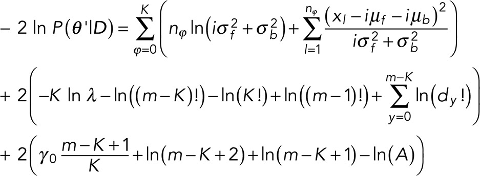
We now insert the full prior from Eq. 19 and the likelihood from Eq. 1 into the formula for the posterior from Eq. 3 and integrate over all μ’s and σ’s. Rather than maximizing the resulting marginal posterior that we obtain from this procedure, we can minimize its negative logarithm (which, for the sake of comparison to typical information criteria, we multiply by a factor of 2). Up to constant factors, which are irrelevant in model comparison, we obtain
 (20) (20)
|
where 
This equation appears as Eq. 11 in the text.
Acknowledgments
We thank Kristofor Nyquist, Jae Yen Shin, and Andreas Martin for interesting discussions. We also thank the Walczak group (Indiana University, Bloomington, IN), the Peterman and Wuite groups (Vrije Universiteit Amsterdam, Amsterdam, Netherlands), the Lee and Benkovic groups (Pennsylvania State University, State College, PA), and the Steel and Gafni groups (University of Michigan, Ann Arbor, MI) for kindly supplying us with experimental data sets on which to test our algorithm. S.P. acknowledges support from the National Science Foundation (MCB Award 1412259) and his Indiana University–Purdue University Indianapolis start-up for new investigators. N.G.W. acknowledges partial support from National Institutes of Health grants R01 GM081025 and R21 AI109791.
Abbreviations used:
- AIC
Akaike information criterion
- aSNR
adjusted signal-to-noise ratio
- DDS
drug delivery systems
- GFP
green fluorescent protein
- HILO
highly inclined and laminated optical sheet
- HMMs
hidden Markov models
- HPLC
high-performance liquid chromatography
- MCAK
mitotic centromere–associated kinase
- NHS
N-hydroxysuccinimide
- OF
offset
- OSS
oxygen scavenger system
- PALM
photoactivated localization microscopy
- PBS
phosphate-buffered saline
- PR
precision
- ROI
region of interest
- SE
sensitivity
- SIC
Schwartz information criterion
- SNR
signal-to-noise ratio
- SONIC
spot number intensity correlation.
Footnotes
This article was published online ahead of print in MBoC in Press (http://www.molbiolcell.org/cgi/doi/10.1091/mbc.E16-06-0404) on September 21, 2016.
REFERENCES
- Akaike H. A new look at the statistical model identification. IEEE Trans Automatic Control. 1974;19:716–723. [Google Scholar]
- Annibale P, Vanni S, Scarselli M, Rothlisberger U, Radenovic A. Quantitative photo activated localization microscopy: unraveling the effects of photoblinking. PLoS One. 2011;6:e22678. doi: 10.1371/journal.pone.0022678. [DOI] [PMC free article] [PubMed] [Google Scholar]
- Arumugam SR, Lee T-H, Benkovic SJ. Investigation of stoichiometry of T4 bacteriophage helicase loader protein (gp59) J Biol Chem. 2009;284:29283–29289. doi: 10.1074/jbc.M109.029926. [DOI] [PMC free article] [PubMed] [Google Scholar]
- Backlund MP, Lew MD, Backer AS, Sahl SJ, Moerner WE. The role of molecular dipole orientation in single-molecule fluorescence microscopy and implications for super-resolution imaging. ChemPhysChem. 2014;15:587–599. doi: 10.1002/cphc.201300880. [DOI] [PMC free article] [PubMed] [Google Scholar]
- Bagshaw CR, Cherny D. Blinking fluorophores: what do they tell us about protein dynamics? Biochem Soc Trans. 2006;5:979–982. doi: 10.1042/BST0340979. [DOI] [PubMed] [Google Scholar]
- Carter BC, Vershinin M, Gross SP. A comparison of step-detection methods: how well can you do? Biophys J. 2008;94:306–319. doi: 10.1529/biophysj.107.110601. [DOI] [PMC free article] [PubMed] [Google Scholar]
- Cavanaugh JE, Neath AA. Generalizing the derivation of the Schwarz information criterion. Commun Stat Theory Methods. 1999;28:49–66. [Google Scholar]
- Chen Y, Deffenbaugh NC, Anderson CT, Hancock WO. Molecular counting by photobleaching in protein complexes with many subunits: best practices and application to the cellulose synthesis complex. Mol Biol Cell. 2014;25:3630–3642. doi: 10.1091/mbc.E14-06-1146. [DOI] [PMC free article] [PubMed] [Google Scholar]
- Claeskens G, Hjort NL. Model Selection and Model Averaging. Cambridge, UK: Cambridge University Press; 2008. [Google Scholar]
- Coffman VC, Wu J-Q. Counting protein molecules using quantitative fluorescence microscopy. Trends Biochem Sci. 2012;37:499–506. doi: 10.1016/j.tibs.2012.08.002. [DOI] [PMC free article] [PubMed] [Google Scholar]
- Coffman VC, Wu P, Parthun MR, Wu J-Q. CENP-A exceeds microtubule attachment sites in centromere clusters of both budding and fission yeast. J Cell Biol. 2011;195:563–572. doi: 10.1083/jcb.201106078. [DOI] [PMC free article] [PubMed] [Google Scholar]
- Das SK, Darshi M, Cheley S, Wallace MI, Bayley H. membrane protein stoichiometry determined from the step-wise photobleaching of dye-labelled subunits. ChemBioChem. 2007;8:994–999. doi: 10.1002/cbic.200600474. [DOI] [PubMed] [Google Scholar]
- Delalez NJ, Wadhams GH, Rosser G, Xue Q, Brown MT, Dobbie IM, Berry RM, Leake MC, Armitage JP. Signal-dependent turnover of the bacterial flagellar switch protein FliM. Proc Natl Acad Sci USA. 2010;107:11347–11351. doi: 10.1073/pnas.1000284107. [DOI] [PMC free article] [PubMed] [Google Scholar]
- Demuro A, Penna A, Safrina O, Yeromin AV, Amcheslavsky A, Cahalan MD, Parker I. Subunit stoichiometry of human Orai1 and Orai3 channels in closed and open states. Proc Natl Acad Sci USA. 2011;108:17832–17837. doi: 10.1073/pnas.1114814108. [DOI] [PMC free article] [PubMed] [Google Scholar]
- Durisic N, Laparra-Cuervo L, Sandoval-Álvarez Á, Borbely JS, Lakadamyali M. Single-molecule evaluation of fluorescent protein photoactivation efficiency using an in vivo nanotemplate. Nat Methods. 2014;11:156–162. doi: 10.1038/nmeth.2784. [DOI] [PubMed] [Google Scholar]
- Drobizhev M, Hughes TE, Stepanenko Y, Wnuk P, O’Donnell K, Scott JN, Callis PR, Mikhaylov A, Dokken L, Rebane A. Primary role of the chromophore bond length alternation in reversible photoconversion of red fluorescence proteins. Sci Rep. 2012;2:688. doi: 10.1038/srep00688. [DOI] [PMC free article] [PubMed] [Google Scholar]
- Ems-McClung SC, Hainline SG, Devare J, Zong H, Cai S, Carnes SK, Shaw SL, Walczak CE. Aurora B inhibits MCAK activity through a phosphoconformational switch that reduces microtubule association. Curr Biol. 2013;23:2491–2499. doi: 10.1016/j.cub.2013.10.054. [DOI] [PMC free article] [PubMed] [Google Scholar]
- Engel BD, Ludington WB, Marshall WF. Intraflagellar transport particle size scales inversely with flagellar length: revisiting the balance-point length control model. J Cell Biol. 2009;187:81–89. doi: 10.1083/jcb.200812084. [DOI] [PMC free article] [PubMed] [Google Scholar]
- Gillespie D. Exact stochastic simulation of coupled chemical reactions. J Phys Chem. 1977;81:2340–2361. [Google Scholar]
- Ha T, Tinnefeld P. Photophysics of fluorescent probes for single-molecule biophysics and super-resolution imaging. Annu Rev Phys Chem. 2012;63:595–617. doi: 10.1146/annurev-physchem-032210-103340. [DOI] [PMC free article] [PubMed] [Google Scholar]
- Hastie P, Ulbrich MH, Wang H-L, Arant RJ, Lau AG, Zhang Z, Isacoff EY, Chen L. AMPA receptor/TARP stoichiometry visualized by single-molecule subunit counting. Proc Natl Acad Sci USA. 2013;110:5163–5168. doi: 10.1073/pnas.1218765110. [DOI] [PMC free article] [PubMed] [Google Scholar]
- Kadane JB, Lazar NA. Methods and criteria for model selection. J Am Stat Assoc. 2004;99:279–290. [Google Scholar]
- Kalafut B, Visscher K. An objective, model-independent method for detection of non-uniform steps in noisy signals. Comput Phys Commun. 2008;179:716–723. [Google Scholar]
- Kerssemakers JWJ, Munteanu EL, Laan L, Noetzel TL, Janson ME, Dogterom M. Assembly dynamics of microtubules at molecular resolution. Nature. 2006;442:709–712. doi: 10.1038/nature04928. [DOI] [PubMed] [Google Scholar]
- Lawrimore J, Bloom KS, Salmon ED. Point centromeres contain more than a single centromere-specific Cse4 (CENP-A) nucleosome. J Cell Biol. 2011;195:573–582. doi: 10.1083/jcb.201106036. [DOI] [PMC free article] [PubMed] [Google Scholar]
- Leake MC, Chandler JH, Wadhams GH, Bai F, Berry RM, Armitage JP. Stoichiometry and turnover in single, functioning membrane protein complexes. Nature. 2006;443:355–358. doi: 10.1038/nature05135. [DOI] [PubMed] [Google Scholar]
- Lee S-H, Shin JY, Lee A, Bustamante C. Counting single photoactivatable fluorescent molecules by photoactivated localization microscopy (PALM) Proc Natl Acad Sci USA. 2012;109:17436–17441. doi: 10.1073/pnas.1215175109. [DOI] [PMC free article] [PubMed] [Google Scholar]
- Liesche C, Grußmayer K, Ludwig M, Wörz S, Rohr K, Herten D-P, Beaudouin J, Eils R. Automated analysis of single-molecule photobleaching data by statistical modeling of spot populations. Biophys J. 2015;109:2352–2362. doi: 10.1016/j.bpj.2015.10.035. [DOI] [PMC free article] [PubMed] [Google Scholar]
- Lippincott-Schwartz J, Altan-Bonnet N, Patterson G. Photobleaching and photoactivation: following protein dynamics in living cells. Nat Cell Biol. 2003;5:S7–S14. [PubMed] [Google Scholar]
- Llorente-Garcia I, Lenn T, Erhardt H, Harriman OL, Liu L-N, Robson A, Chiu S-W, Matthews S, Willis NJ, Bray CD, et al. Single-molecule in vivo imaging of bacterial respiratory complexes indicates delocalized oxidative phosphorylation. Biochim Biophys Acta. 2014;1837:811–824. doi: 10.1016/j.bbabio.2014.01.020. [DOI] [PubMed] [Google Scholar]
- Ludden TM, Beal SL, Sheiner LB. Comparison of the Akaike information criterion, the Schwarz criterion and the F test as guides to model selection. J Pharmacokinet Biopharm. 1994;22:431–445. doi: 10.1007/BF02353864. [DOI] [PubMed] [Google Scholar]
- McGuire H, Aurousseau MRP, Bowie D, Blunck R. Automating single subunit counting of membrane proteins in mammalian cells. J Biol Chem. 2012;287:35912–35921. doi: 10.1074/jbc.M112.402057. [DOI] [PMC free article] [PubMed] [Google Scholar]
- Messina TC, Kim H, Giurleo JT, Talaga DS. Hidden Markov model analysis of multichromophore photobleaching. J Phys Chem B. 2006;110:16366–16376. doi: 10.1021/jp063367k. [DOI] [PMC free article] [PubMed] [Google Scholar]
- Monici M. Cell and tissue autofluorescence research and diagnostic applications. Biotechnol Annu Rev. 2005;11:227–256. doi: 10.1016/S1387-2656(05)11007-2. [DOI] [PubMed] [Google Scholar]
- Pitchiaya S, Androsavich JR, Walter NG. Intracellular single molecule microscopy reveals two kinetically distinct pathways for microRNA assembly. EMBO Rep. 2012;13:709–715. doi: 10.1038/embor.2012.85. [DOI] [PMC free article] [PubMed] [Google Scholar]
- Pitchiaya S, Heinicke LA, Custer TC, Walter NG. Single molecule fluorescence approaches shed light on intracellular RNAs. Chem Rev. 2014;114:3224–3265. doi: 10.1021/cr400496q. [DOI] [PMC free article] [PubMed] [Google Scholar]
- Pitchiaya S, Krishnan V, Custer TC, Walter NG. Dissecting non-coding RNA mechanisms in cellulo by single-molecule high-resolution localization and counting. Methods. 2013;63:188–199. doi: 10.1016/j.ymeth.2013.05.028. [DOI] [PMC free article] [PubMed] [Google Scholar]
- Pressé S, Ghosh K, Lee J, Dill KA. Principles of maximum entropy and maximum caliber in statistical physics. Rev Mod Phys. 2013;85:1115–1141. [Google Scholar]
- Rollins GC, Shin JY, Bustamante C, Pressé S. Stochastic approach to the molecular counting problem in superresolution microscopy. Proc Natl Acad Sci USA. 2015;112:E110–E118. doi: 10.1073/pnas.1408071112. [DOI] [PMC free article] [PubMed] [Google Scholar]
- Schwarz G. Estimating the dimension of a model. Ann Statist. 1978;6:461–464. [Google Scholar]
- Shankar S, Pitchiaya S, Malik R, Kothari V, Hosono Y, Yocum A, Gundlapalli H, White Y, Firestone A, Cao X, et al. KRAS engages AGO2 to enhance cellular transformation. Cell Rep. 2016;14:1448–1461. doi: 10.1016/j.celrep.2016.01.034. [DOI] [PMC free article] [PubMed] [Google Scholar]
- Shu D, Zhang H, Jin J, Guo P. Counting of six pRNAs of phi29 DNA-packaging motor with customized single-molecule dual-view system. EMBO J. 2007;26:527–537. doi: 10.1038/sj.emboj.7601506. [DOI] [PMC free article] [PubMed] [Google Scholar]
- Stoica P, Selen Y. Model-order selection: a review of information criterion rules. IEEE Signal Proc Mag. 2004;21:36–47. [Google Scholar]
- Sung P, Krejci L, Van Komen S, Sehorn MG. Rad51 recombinase and recombination mediators. J Biol Chem. 2003;278:42729–42732. doi: 10.1074/jbc.R300027200. [DOI] [PubMed] [Google Scholar]
- Svoboda K, Schmidt CF, Schnapp BJ, Block SM. Direct observation of kinesin stepping by optical trapping interferometry. Nature. 1993;365:721–727. doi: 10.1038/365721a0. [DOI] [PubMed] [Google Scholar]
- Tavakoli M, Taylor JN, Li C-B, Komatsuzaki T, Pressé S. Single molecule data analysis: an introduction. 2016. arXiv:1606.00403 [physics, q-bio]
- Ulbrich MH, Isacoff EY. Subunit counting in membrane-bound proteins. Nat Methods. 2007;4:319–321. doi: 10.1038/NMETH1024. [DOI] [PMC free article] [PubMed] [Google Scholar]
- van Mameren J, Modesti M, Kanaar R, Wyman C, Peterman EJG, Wuite GJL. Counting RAD51 proteins disassembling from nucleoprotein filaments under tension. Nature. 2009;457:745–748. doi: 10.1038/nature07581. [DOI] [PMC free article] [PubMed] [Google Scholar]
- Walczak CE, Gayek S, Ohi R. Microtubule-depolymerizing kinesins. Annu Rev Cell Dev Biol. 2013;29:417–441. doi: 10.1146/annurev-cellbio-101512-122345. [DOI] [PubMed] [Google Scholar]
- Watanabe S, Punge A, Hollopeter G, Willig KI, Hobson RJ, Davis MW, Hell SW, Jorgensen EM. Protein localization in electron micrographs using fluorescence nanoscopy. Nat Methods. 2011;8:80–84. doi: 10.1038/nmeth.1537. [DOI] [PMC free article] [PubMed] [Google Scholar]
- White J, Stelzer E. Photobleaching GFP reveals protein dynamics inside live cells. Trends Cell Biol. 1999;9:61–65. doi: 10.1016/s0962-8924(98)01433-0. [DOI] [PubMed] [Google Scholar]
- Xia T, Li N, Fang X. Single-molecule fluorescence imaging in living cells. Annu Rev Phys Chem. 2013;64:459–480. doi: 10.1146/annurev-physchem-040412-110127. [DOI] [PubMed] [Google Scholar]