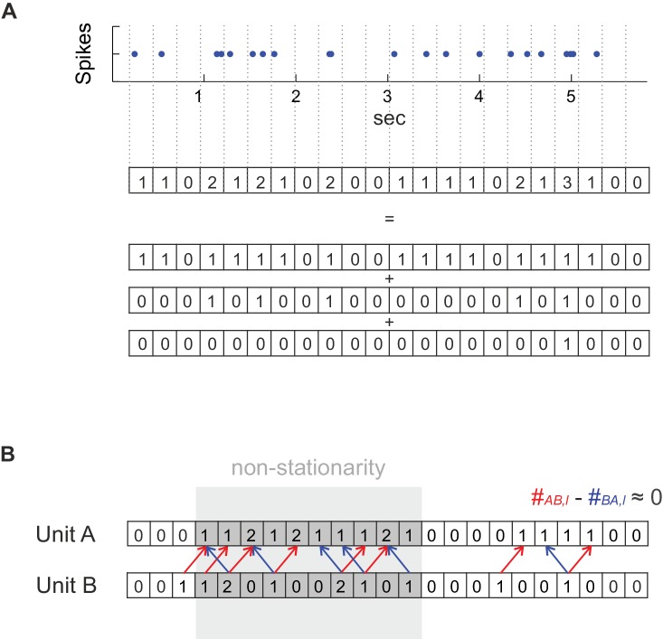
Figure 6. Method details.

(A) For deriving a statistical test that works with any temporal bin width the spike count series were separated into an overlay of several (dependent) binary sub-processes. See Materials and methods for further explanation. (B) Dealing with non-stationarity in the spike trains. In the case of non-stationarity in the form of a common rate increase in two units A and B (highlighted in gray), some spike co-occurrences caused by the rate increase might be incorrectly attributed to coupled activity (mutual dependence) at the finer timescale (bin width) at which coupling is investigated (at a lag of one in the illustrated example), even if there is not really any such coupling as assumed in this example. This corruption by non-stationarity may be removed by considering the difference count ${\displaystyle {\mathrm{\#}}_{AB}-{\mathrm{\#}}_{BA}}$, in which spurious excess coincidences in one direction (${\displaystyle {\mathrm{\#}}_{AB}}$: red arrows) would cancel out with those in the reverse direction (${\displaystyle {\mathrm{\#}}_{BA}}$: blue arrows). It is important to note that if, on the other hand, the rate increase is on the timescale of interest, as it is the case for the ‘rate assemblies’ of type IV or V in Figure 1), subtracting off the reverse-lag count would not prevent assembly detection on that time scale.

DOI: http://dx.doi.org/10.7554/eLife.19428.011

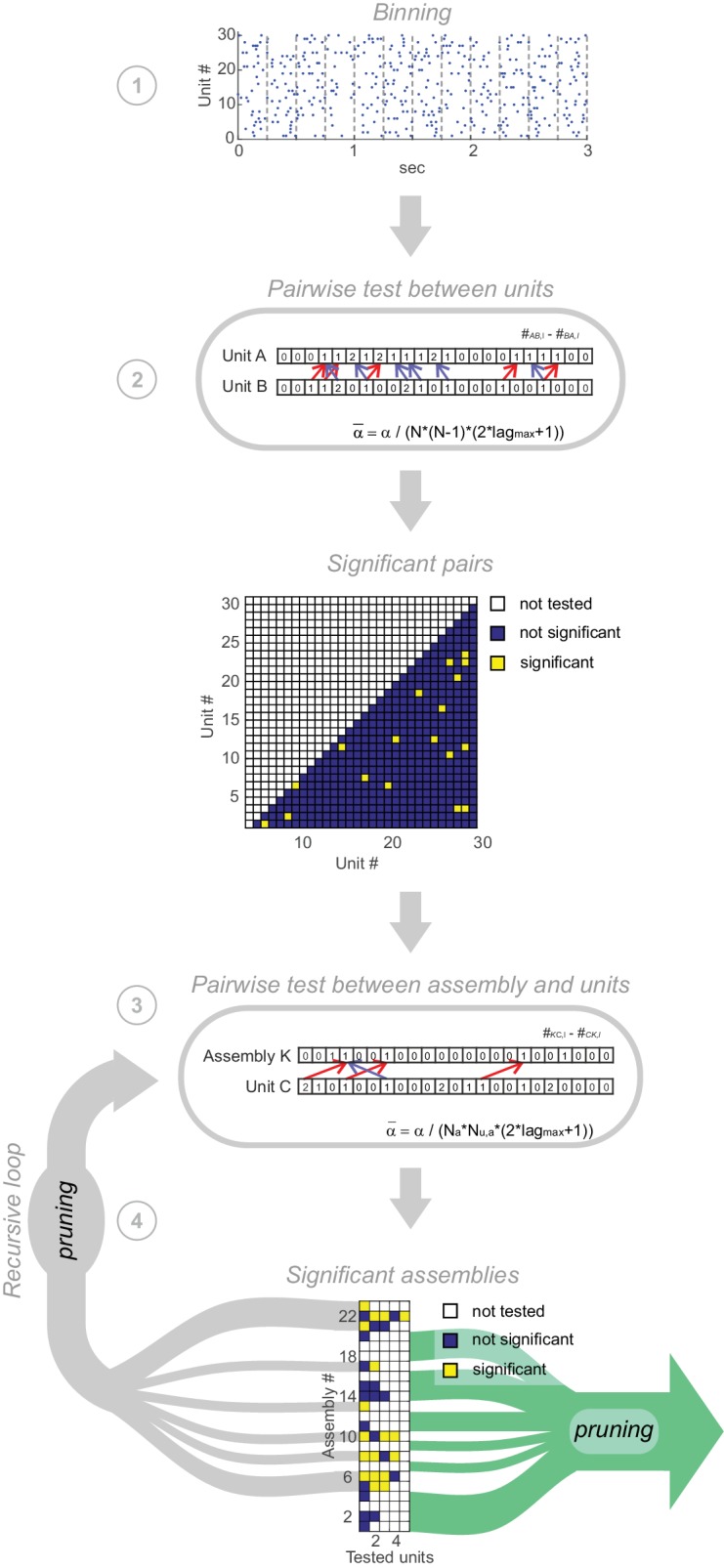
Figure 6—figure supplement 1. Pipeline of assembly agglomeration algorithm.

(1) Binning: Spike trains are binned at some time scale ${\displaystyle \mathrm{\Delta }}$ of interest. (2) Detection of pairwise interactions at chosen scale ${\displaystyle \mathrm{\Delta }}$: For all unit pairs, test ${\displaystyle {\mathrm{\#}}_{AB,\overline{l}}-{\mathrm{\#}}_{AB,-\overline{l}}}$ for significance, with ${\displaystyle \overline{l}\equiv {\mathrm{a}\mathrm{r}\mathrm{g}\mathrm{m}\mathrm{a}\mathrm{x}}_l({\mathrm{\#}}_{AB,l})}$. Significant unit pairs form elementary assemblies fed into the agglomerative recursion loop. (3) Assembly agglomeration: Test pairwise combinations of previously formed assemblies (with time stamps centered on first activated assembly unit) and single units for significance, and add latter to assembly set if significant. For this step, only units are considered which already are significantly related to at least one assembly member. (4) Recursive loop and pruning: All assemblies extended in the previous iteration are fed back into step 3. After each iteration, from all assemblies consisting of the same set of units but with different patterns of time lags only the one with the lowest p-value is retained. The loop is terminated if no units have been added to existing assemblies in the previous iteration. In a final pruning step all assemblies which are true subsets of larger assemblies are removed.

DOI: http://dx.doi.org/10.7554/eLife.19428.012