The Mechanics of Surface Expansion Anisotropy in Medicago truncatula Root Hairs

Abstract

Wall expansion in tip-growing cells shows variations according to position and direction. In Medicago truncatula root hairs, wall expansion exhibits a strong meridional gradient with a maximum near the pole of the cell. Root hair cells also show a striking expansion anisotropy, i.e. over most of the dome surface the rate of circumferential wall expansion exceeds the rate of meridional expansion. Concomitant measurements of expansion rates and wall stresses reveal that the extensibility of the cell wall must vary abruptly along the meridian of the cell to maintain the gradient of wall expansion. To determine the mechanical basis of expansion anisotropy, we compared measurements of wall expansion with expansion patterns predicted from wall structural models that were either fully isotropic, transversely isotropic, or fully anisotropic. Our results indicate that a model based on a transversely isotropic wall structure can provide a good fit of the data although a fully anisotropic model offers the best fit overall. We discuss how such mechanical properties could be controlled at the microstructural level.

Tip growth is the primary mode of morphogenesis for a wide range of cells including some prokaryotes (e.g. Streptomycetes), fungal hyphae, certain unicellular algae, pollen tubes, and root hairs (see articles in Heath, 1990). The shape of tip-growing cells is characterized by a long cylinder capped with a prolate dome. Evidence that cell wall expansion is limited to the dome was first obtained by Haberlandt (1887) and Reinhardt (1892) who, respectively, used starch grains and red lead particles to mark the cell surface. Since then, refined marking protocols and improved microscopic techniques have established two fundamental features of wall expansion during tip growth (Castle, 1958; Green, 1965; Chen, 1973; Hejnowicz et al., 1977; Kataoka, 1982; Shaw et al., 2000; von Dassow et al., 2001). First, the rate of wall expansion is distributed in a meridional gradient with a maximum at or near the pole of the dome and minimum at the equator. Wall expansion is therefore inhomogeneous. Second, over most of the dome surface wall expansion in the circumferential direction exceeds expansion in the meridional direction. Wall expansion is therefore anisotropic.

To explain these observations, we must consider the cellular control of wall expansion. Wall expansion is commonly interpreted as a mechanical deformation (Heyn, 1940; Ekdahl, 1953; Green, 1965; Lockhart, 1965a, 1965b; Hejnowicz et al., 1977; Ray, 1987; Cosgrove, 1993). According to this view, the relative elemental rate of wall expansion or strain rate is determined by two mechanical factors: the turgor-induced stresses present in the cell wall and the local mechanical properties of the wall. Variations in the wall strain rates, whether between different locations or different directions, must ultimately be traced back to variations in one of these two controlling factors.

Ever since Reinhardt's work (1892), it is known that the meridional gradient of wall expansion observed in tip-growing cells does not reflect a similar gradient of wall stresses. In fact, the wall stresses predicted for the dome of the cell follow a gradient opposite to the observed gradient of expansion (Reinhardt, 1892; Hejnowicz et al., 1977; but see also von Dassow et al., 2001). This seemingly paradoxical observation can be explained if the wall mechanical properties are themselves varying in such a way that the cell wall in the polar region of the dome is highly extensible while the cell wall at the base of the dome is not. According to Green (1973) and Hejnowicz et al. (1977), a gradient of mechanical properties can be established if the newly secreted wall material is initially extensible but gradually stiffens in response to stretching, a phenomenon known as strain hardening. This model explains the gradient of mechanical properties exclusively in physical terms. The graded mechanical properties could also be under more direct cellular or molecular control. For example, sustained deposition of cellulose microfibrils followed by cross-linking of the microfibrils could lead to a stiffening of the cell wall material. Such mechanisms have been proposed many times, most notably by Ekdahl (1953) for root hairs and by Wessels (1986, 1988) for fungal hyphae where the alleged cross-linking now occurs between chitin microfibrils.

The control of expansion anisotropy was studied extensively in diffusely growing cells such as the Nitella internodal cell but not in tip-growing cells. In the cylindrical Nitella cell, the axial rate of wall extension is four times the circumferential rate of extension, whereas the axial stress is only one-half the circumferential stress (Green, 1963). Again, this paradoxical observation is explained if the mechanical properties in the plane of the cell wall are varying with direction. A frequently cited explanation for expansion anisotropy in diffusely growing cells is a mechanical anisotropy of the cell wall matrix provided by circumferentially oriented cellulose microfibrils (Green, 1962; Probine and Preston, 1962; Probine, 1966; Richmond et al., 1980; Sellen, 1983). The cellulose reinforcement prevents extension in the circumferential direction despite the greater stress in that direction (Fig. 1A). The deposition of cellulose microfibrils is believed to be guided by circumferentially oriented cortical microtubules (Lloyd, 1984). If the preferential orientation of cellulose microfibrils is perturbed, the expansion anisotropy is lost and the cell soon adopts a spherical shape (Green, 1962).

Figure 1.

A, Two alternatives for anisotropic wall expansion. In Nitella, stresses (solid arrows) favor transverse extension, but high mechanical anisotropy of the cell wall leads ultimately to axial extension. For tip-growing cells, we postulate that the cell wall has no intrinsic mechanical anisotropy in its plane so that expansion anisotropy reflects solely the bias in the wall stresses. B, Geometry of a tip-growing cell. The plane stresses (σ) acting on a small wall element are shown along with the strain rates () they produce.

We can ask whether the anisotropy of wall expansion in tip-growing cells depends, as for diffusely growing cells, on structural anisotropy in the cell wall. Studies of wall structure at the dome of various tip-growing cells have all reported a random orientation of cellulose microfibrils (Houwink and Roelofsen, 1954; O'Kelley and Carr, 1954; Belford and Preston, 1961; Newcomb and Bonnett, 1965; Chen, 1980; Kataoka, 1982). The lack of specific microfibril orientation suggests that the mechanical properties are isotropic in the plane of the cell wall. One implication of this observation is that expansion anisotropy in tip-growing cells may arise from stress anisotropy and not from directional reinforcement of the cell wall as observed in diffusely growing cells (Fig. 1A).

A recent investigation of tip growth in Medicago truncatula root hairs (Shaw et al., 2000) provided the basic quantitative data necessary to analyze the mechanics of tip growth in detail. The goal of this paper is to perform a mechanical analysis of tip growth that includes measurements of strain rates and stresses and estimates for the mechanical properties of the cell wall. In particular, we will test whether the mechanical model suggested by the wall structure of tip-growing cells is sufficient to explain the observed pattern of wall expansion.

RESULTS

Our results are based on a reanalysis of data collected on four actively growing root hairs of the legume Medicago truncatula (Shaw et al., 2000). Cell numbers 1 to 4 in this paper correspond to cells D, C, A, and B in Figure 4 of Shaw et al. (2000). Using time-lapse imaging of root hairs labeled with fluorescent microspheres, it was possible to record the geometry of the cell and the expansion of the cell surface over a period of 30 to 45 min. Figures 2A and 3A illustrate the raw data on which this work is based.

Figure 4.

Meridional distribution of wall stresses and strain rates for two root hairs of M. truncatula. The left-hand and right-hand sections are for cell number 1 and cell number 2, respectively. A and B, Wall stresses inferred from the cell geometry. C and D, Strain rates derived from the best fit of the velocity data for n = 3. E and F, Predicted strain rates for a transversely isotropic cell wall. The shaded areas highlight the regions where the meridional stress exceeds the circumferential stress.

Figure 2.

Raw data for cell number 1. A, Growth sequence of a M. truncatula root hair. The cell outline is shown at 3-min time intervals. The fiducial points used to define the cell geometry are highlighted on the last outline of the sequence. The position of surface markers (fluorescent microspheres) is also shown before (stars) and after (circles) projection onto the cell outlines. The axis of growth is the solid line following the pole of the cell through the entire sequence. Trajectories perpendicular to the cell outlines are indicated by dashed curves. B, Average κ_s for the cell. The observed mean and sd are shown at various locations. The solid line is the best fit of these data. C, Meridional velocity of surface markers shown in A. The solid line is the best fit of these data for n = 3 (see text).

Figure 3.

Raw data for cell number 2. Legend as for Figure 2.

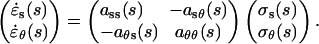
A mechanical analysis of tip growth must begin with measurements of two types of variables: the relative elemental rates of wall expansion or strain rates () and the turgor-induced wall stresses (σ). The strain rates and stresses are defined along three principal directions (s, θ, and n) corresponding to the meridional, circumferential, and normal directions on a dome (Fig. 1B). Our analysis focuses on the strain rates and stresses in the meridional and circumferential directions only because current experimental protocols do not allow us to measure these variables in the normal direction. Inspection of the time-lapse sequences in Figures 2A and 3A reveals that the cell geometry and the rate of elongation are relatively constant. Given these two features, it is possible to pool the data collected over the entire growth sequence and to express the stresses and strain rates associated with tip growth in terms of only two independent variables: the meridional curvature (κ_s) of the cell and the meridional velocity of material points (v; see Eqs. 1 and 2, and 4 and 5 in “Materials and Methods” section).

Tip Geometry and Wall Stresses

The fiducial points marking the cell outlines (Figs. 2A and 3A) were used to compute κ_s. The measured κ_s shows two distinct maxima approximately 3 microns from the pole of the cell (Figs. 2B and 3B). Based on this observation, Shaw et al. (2000) defined three zones on the dome: a polar cap 1 to 2 microns wide, a surrounding annulus of high curvature, and flanks of steadily decreasing curvature.

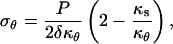
The wall stresses computed from the cell geometry (Eqs. 1 and 2) are shown in Figure 4, A and B. The meridional and circumferential stresses are identical at the pole of the cell. While the meridional stress shows only small deviations from its value at the pole, the circumferential stress first decreases slightly below the meridional stress and then increases steadily to reach, at the equator, a value that is nearly twice that of the meridional stress. In the cylindrical portion of the cell, where κ_s falls to zero, the circumferential stress is predicted to be exactly twice the meridional stress (simply substitute in Eqs. 1 and 2). We conclude that over most of the tip surface, the wall stresses favor a circumferential expansion of the cell surface.

Velocity of Material Points and Strain Rates

The displacement of fluorescent microspheres was used to compute the v as shown in Figures 2C and 3C. These data were fitted with a function of the form where is a polynomial whose degree n should be selected carefully. Increasing the number of terms in improves the fit of the data and can ultimately lead to a perfect fit if the number of free terms equals the number of data points. This fit would, however, be meaningless given the noise in the data. Therefore, we need to determine the maximum power of the polynomial that has statistical significance. This was done by recording the sum of squared residuals (SSR) associated with different least squares fits of the data (Table I). A low SSR indicates that more of the variation in the data is explained by the fitting function. F-tests were performed to determine whether the inclusion of a given term in the polynomial leads to a reduction in SSR that is statistically significant (see Eq. 3 in “Materials and Methods”; Snedecor and Cochran, 1967; Zar, 1996). In Table I, all F values above 6.90 have a significance level of α = 0.01 or better. According to the forward selection criterion (Zar, 1996), terms should be included until we reach the first term whose reduction in SSR is not statistically significant. Based on the trend observed in Table I, n = 3 appears to be an adequate cutoff since F values for n = 4 are not significant for three out of four cells. Note that higher order terms (n ≥ 4) with significant F values are associated with noise in the data.

Table I.

Sum of the squared residuals (SSR) for fits of the velocity data with different powers n of the function

Cell	n = 0a	n = 2	n = 3	n = 4	n = 5	Nd
No. 1	0.319b (100)	0.183 (57)	0.141 (44)	0.139 (44)	0.134 (42)	193
F valuesc		143	55.4	2.71	8.02
No. 2	0.159 (100)	0.0532 (33)	0.0470 (30)	0.0418 (26)	0.0409 (26)	102
F values		199	13.1	12.2	2.13
No. 3	0.341 (100)	0.269 (79)	0.162 (47)	0.159 (47)	0.145 (42)	175
F values		46.5	113	3.45	16.3
No. 4	0.305 (100)	0.130 (43)	0.112 (37)	0.112 (37)	0.0989 (32)	117
F values		155	18.5	0.203	14.4

^an indicates the highest power used in the polynomial . For n = 0, represents a constant. Note also that the first power is excluded from the polynomial for reasons of compatibility (see “Materials and Methods” section).

^bThe SSR is measured in (μm/min)². Numbers in parentheses are percent SSR based on the value for n = 0.

^cAll F values that exceed 6.90 are significant to α = 0.01.

^dN is the number of data points.

Strain rates were computed from Equations 4 and 5 and our fit of the velocity data for n = 3 (Fig. 4, C and D). The inhomogeneity and anisotropy of wall expansion mentioned in the introduction are here quantified. Near the pole of the cell, the two rates of wall extension are approximately 8%/min, while 5 microns away from the pole the circumferential and meridional rates have, respectively, dropped to 5% and 2%/min. An alternative, but equivalent, statement is that the apical region within 5 microns of the pole contributes 55% to 60% of the total increase in wall surface area. Wall expansion anisotropy also varies on the dome. The meridional extension rate can exceed the circumferential rate near the pole of the cell, although the most salient feature of the strain anisotropy are the long shoulders where wall extension in the circumferential direction is dominant.

Wall Mechanical Properties

The mechanical properties of the cell wall can be inferred from a comparison of the strain rates and wall stresses. We first note that the mean in-plane stress increases away from the pole, while the strain rates show an overall decline. This discrepancy suggests that there is a meridional gradient of mechanical properties. An estimate of wall extensibility is given by the ratio 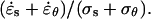As illustrated in Figure 5, wall extensibility shows a sharp gradient with the most extensible cell wall located within 5 microns of the pole.

Figure 5.

Predicted cell wall extensibility for cell number 1 (solid line) and cell number 2 (dashed line).

The mechanical anisotropy that may be present in the cell wall defies any simple measurement and is best evaluated by comparison with explicit models of wall structure. We consider three different wall structures and their corresponding set of mechanical properties (Fig. 6A; Table II). The first model is a wall with randomly oriented cellulose microfibrils. Given the lack of structure in such a cell wall, we may expect isotropic mechanical properties between all three principal directions. The second model is inspired by observations of wall structure in tip-growing cells where cellulose microfibrils are organized into layers parallel to the cell surface but have no preferential orientation within a layer (Fig. 6A). This structure emerges naturally from wall assembly since cellulose microfibrils are synthesized by enzyme complexes that travel along the cell membrane. This wall organization suggests that the mechanical properties can be isotropic in the cell wall plane but that they are likely to differ from the mechanical properties in the direction normal to the cell surface. We shall refer to this model as transverse isotropy. Finally, we consider also a fully anisotropic cell wall with different mechanical properties in the three principal directions. This type of cell wall is characteristic of diffusely growing cells such as the Nitella internodal cell and reflects a highly organized deposition of cellulose microfibrils within the plane of the wall (Fig. 6A).

Figure 6.

A, Models of cell wall structure showing the distribution of cellulose microfibrils within a wall element. For transversely isotropic and fully anisotropic models, cellulose microfibrils are confined to layers (s-θ planes) parallel to the cell surface. B, Anisotropy space. The stress and strain anisotropy for an isotropic material must lie on the line λ = 3γ (dotted line), while those for a transversely isotropic material must lie in the shaded area. The stress and strain anisotropy for a fully anisotropic material can occupy any point in the anisotropy space. The measured stress and strain anisotropy for cell number 1 and cell number 2 are shown (solid lines). The approximate meridional positions where the strain rates and stresses were measured are indicated. It can be seen that the data deviate from the region of transverse isotropy near to origin. The strain and stress anisotropy for the transversely isotropic model that best fit the data are shown (dashed lines). The strain and stress anisotropy observed in Nitella and Hydrodictyon (Green, 1963) are also included for comparison.

Table II.

Constraints on the mechanical properties and strain anisotropy according to three structural models of the cell wall

Structural Models	Mechanical Propertiesa	Anisotropy
Isotropy	ass = aθθ = 2asθ = 2aθs	λ = 3γ
(s = θ = n)b
Transverse isotropy	ass = aθθ	λ ≥ γ for γ > 0
(s = θ ≠ n)	asθ = aθs	λ ≤ γ for γ < 0
		λ = 0 for γ = 0
Anisotropy	asθ = aθs	λ not constrained by γ
(s ≠ θ ≠ n)	ass and aθθ are free

^aSee “Materials and Methods” section for additional information on the mechanical properties.

^bAn equal sign indicates directions that are mechanically equivalent.

The models impose specific constraints on the pattern of strains that can be observed. To visualize these constraints, we must first introduce two ratios: the strain anisotropy, 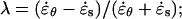and the stress anisotropy, 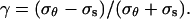These two ratios define a space of possible anisotropy (Fig. 6B). As indicated in Table II, the strain and stress anisotropy for an isotropic cell wall must lie on a straight line in the anisotropy space. Strain and stress anisotropy for a transversely isotropic cell wall can cover a larger subset of the anisotropy space (shaded area in Fig. 6B). Finally, an anisotropic cell wall can lead to any combination of stress and strain anisotropy.

The observed strain and stress anisotropy for cell number 1 and cell number 2 were plotted in the anisotropy space (Fig. 6B). The data deviate from the line corresponding to a fully isotropic model and also slightly from the region accessible to a transversely isotropic model. The deviation near the origin indicates that meridional stiffening is present in the plane of the cell wall. For comparison, we also included stress and strain anisotropy measurements for the Nitella internodal cell and Hydrodictyon, both of which show strong structural anisotropy in their wall. The measurements lie squarely outside the subspace accessible to an isotropic or transversely isotropic model confirming that these simpler structural models offer a poor description of the mechanical anisotropy present in the wall of these cells.

To go beyond the qualitative conclusions that emerge from inspection of the anisotropy space, we also fitted the velocity data directly with functions compatible with the three structural models (see “Materials and Methods” section). The simplest model that offers a good quantitative fit can be retained as the best candidate for the wall structure. Goodness-of-fit was measured with the SSR associated with each model (Table III). As already hinted by the plot of Figure 6B, a fully anisotropic model offers the best fit overall. Moreover, F-tests indicate that the improvement over the transversely isotropic model is statistically significant for all cells. We note that the fit for an anisotropic model is the same as the free fit used in the previous section. The strain rates of Figure 4, C and D thus correspond to the anisotropic structural model. We have also determined the strain rates for a transversely isotropic structural model (Fig. 4, E and F). Comparison of the strain rates for the two models indicates that all of the key features of the expansion patterns are retained in the simpler, transversely isotropic model.

Table III.

SSR for fits of the velocity data subjected to constraints from three structural models of the cell wall: isotropy (iso), transverse isotropy (trans), and full anisotropy (aniso)

Cell	p = 1a		p = 3		Nc
		Iso	Trans	Anisob
No. 1	0.528d (100)	0.327 (62)	0.202 (38)	0.141 (27)	193
F valuese		118	119	82.2
No. 2	0.660 (100)	0.186 (28)	0.0551 (8)	0.0470 (7)	102
F values		257	235	17.1
No. 3	0.599 (100)	0.337 (56)	0.278 (46)	0.162 (27)	175
F values		135	36.5	123
No. 4	0.481 (100)	0.257 (53)	0.154 (32)	0.112 (23)	117
F values		101	76.2	42.8

For comparison, a fit of the velocity data that leads to isotropic strain rates () was also included.

^ap indicates the number of free parameters used in the fitting.

^bThe anisotropic model in this table corresponds to the free fit in column n = 3 of Table I.

^cN is the number of data points.

^dThe SSR is measured in (μm/min)². Numbers in parentheses are percent SSR based on the value for the isotropic strain model.

^eAll F values that exceed 6.90 are significant to α = 0.01.

The data presented in Table III can also be used to determine the fraction of the total strain anisotropy explained by a transversely isotropic model. This model has no structural anisotropy in the plane of the wall and thus only stresses can contribute to anisotropy in the expansion of the cell surface. The strain anisotropy present in our data is the amount of variation that cannot be explained by a model with isotropic strains minus the variation that cannot be explained at all (i.e. the variation due to noise). Consequently, a measure of the total strain anisotropy is the SSR for a model with isotropic strains (i.e. ) minus the SSR for the fully anisotropic model that corresponds to the best fit of the data. The latter SSR value is the variation, or noise, not accounted for by any reasonable model. Taking cell number 1 as example, we find that the amount of variation that can be imputed to strain anisotropy is 0.528 − 0.141 = 0.387 (μm/min)². On the other hand, the reduction in SSR for the transversely isotropic model is 0.528 − 0.202 = 0.32 (μm/min)². Thus, we can infer that a transversely isotropic model accounts for 83% of the total strain anisotropy. Similar calculations for cells number 2, number 3, and number 4 give values of 99%, 73%, and 89%, respectively. We conclude that a transversely isotropic model offers a good qualitative and quantitative fit of our data, although the anisotropic model provides the best fit overall.

DISCUSSION

The strain pattern observed in M. truncatula root hairs is similar to that reported for the Chara and Nitella rhizoids (Chen, 1973; Hejnowicz et al., 1977) and for Phycomyces (Castle, 1958). These distantly related organisms show the same predominance of meridional strain rate in the most apical region of the dome with a wider subapical region where the circumferential strain rate exceeds the meridional strain rate. The wide range of cells sharing this strain pattern suggests that it is a fundamental feature of the tip growth process, one that transcends known differences in the chemical composition of the cell wall. With our analysis, we can propose a basis for the wall expansion pattern observed in M. truncatula.

Wall Expansion Gradient

Root hairs and other tip-growing cells show a strong meridional gradient of wall expansion. Using measurements of strain rates and stresses, we were able to infer the wall extensibility necessary to maintain tip growth (Fig. 5). Gradients of wall extensibility have often been postulated but their profile was never quantified. Our measure of wall extensibility, although not definitive, is indicative of the type of mechanical inhomogeneities that can be expected in the wall of tip-growing cells. In particular, one might ask whether the sharp transition between regions of high and low wall extensibility mimics the distribution of wall secretion or some wall components involved in regulating expansion. Such spatial correlations between mechanical properties and wall composition are a key first step toward elucidating the control of wall expansion at the molecular level.

Wall Expansion Anisotropy

Wall expansion anisotropy can arise from only two sources: anisotropy in the stresses driving wall expansion or anisotropy in the mechanical properties of the cell wall. Green and King (1966) and Hejnowicz et al. (1977) have shown experimentally that the type of expansion anisotropy observed in M. truncatula root hairs and other tip-growing cells is also observed in mechanically isotropic elastic membranes provided they adopt the shape typical of tip-growing cells. The explanation presented by these authors is that a uniform pressure applied to a prolate dome creates anisotropic stresses which themselves lead to anisotropic strains. Typically, stresses are isotropic at the pole of the dome because the two curvatures (κ_s and κ_θ) are geometrically constrained to be equal at that location (Eqs. 1 and 2). At the equator, the circumferential stress is twice the meridional stress because κ_s vanishes. Therefore, any structure—whether a plant cell or an elastic membrane—that has for geometry a cylinder capped with a prolate dome will show the kind of stress anisotropy illustrated in Figure 4, A and B. This pattern of stress anisotropy is compatible, at least qualitatively, with the most salient feature of the strain anisotropy, that is, the wide region where circumferential wall extension exceeds meridional extension (Fig. 4, C and D). It is thus plausible that a large fraction of the expansion anisotropy observed in root hairs results from the geometry of the cell and the anisotropic stresses it creates.

The fits with different structural models confirms that a wall with transversely isotropic mechanical properties can provide a good fit of our data (Table III). However, even if the fit is in some cases very good (e.g. cell no. 2), this does not prove that the mechanical properties are transversely isotropic since many fully anisotropic models could have generated the same data. We have also found evidence for a nonnegligible amount of mechanical anisotropy in the plane of the cell wall. For all the cells studied, the pattern of wall expansion is suggestive of meridional reinforcement (Fig. 6B). Studies of wall texture at the dome of tip-growing cells did not report such reinforcement (O'Kelley and Carr, 1954; Belford and Preston, 1961; Newcomb and Bonnett, 1965), but a weak preferential orientation of cellulose microfibrils may have been overlooked given the difficulty inherent to such observations and the lack of any quantitative assessment of wall texture.

Table III indicates that a transversely isotropic model offers a substantially better match for the data than a fully isotropic model. Since the only difference between these two models is the possibility of anisotropy between the plane directions and the normal direction, one may wonder why this type of anisotropy affects in any way the performance of these models in fitting the strain anisotropy present in the plane of the cell wall. The reason is that the deformations along the three principal directions are coupled. This coupling, known as a Poisson's ratio effect for elastic materials, can be demonstrated by stretching a material along one direction leading invariably to contraction in the transverse directions. Therefore, a mechanical change that alters wall deformation in the normal direction will also affect, via this coupling, deformation in the plane directions. It is interesting to note that a type of anisotropy that emerges naturally from the deposition of microfibrils into layers may in itself affect expansion anisotropy in the plane of the cell wall.

Tip Growth versus Diffuse Growth

Our findings suggest some important differences between cell morphogenesis by tip growth and diffuse growth. First, tip growth requires a strong gradient of mechanical properties, while such gradients are not necessary for diffuse growth. Gradients imply polarity and thus one key aspect of tip growth is the maintenance of cell polarity (Bibikova et al., 1999; Hepler et al., 2001). Second, expansion anisotropy for the two modes of cell morphogenesis differ in kind. The strain anisotropy present in tip-growing root hairs is for the most part compatible with the stresses present in the cell wall. For this reason, a transversely isotropic model that has no anisotropy within the cell wall plane can account for more than 75% of the wall expansion anisotropy (compare also C and D, and E and F in Fig. 4). For diffusely growing cells, attempts to predict strain anisotropy from the stress anisotropy provide worse predictions than assuming no strain anisotropy at all. In other words, in Figure 6B the data for Nitella and Hydrodictyon lie closer to the x axis, corresponding to an absence of strain anisotropy, than to the regions for the isotropic and transversely isotropic models. We conclude that diffuse growth is crucially dependent on mechanical anisotropy (Green, 1962), while for tip growth, stress anisotropy can already account for the main features of morphogenesis. The difference between the two modes of morphogenesis is not as extreme as the cases depicted in Figure 1A where expansion anisotropy depends solely on mechanical anisotropy for diffuse growth and solely on stress anisotropy for tip growth. The two alternatives, however, are useful working models for the origin of expansion anisotropy in tip growth and diffuse growth.

MATERIALS AND METHODS

Microscopic Techniques and Numerical Analysis

All observations were made on actively growing root hairs of the legume Medicago truncatula Gaernt. cv Jemalong. Each cell was imaged at 1-min intervals using differential interference contrast (DIC) and fluorescence microscopy as detailed in Shaw et al. (2000). The DIC images were used to determine the cell geometry, while fluorescent microspheres were used to mark the cell surface so that surface expansion could be measured. Examples of the raw data are shown in Figures 2A and 3A.

The numerical analysis of the data was based on algorithms written with Matlab (version 5.2; The MathWorks, Natick, MA). All programs are available from J. Dumais (jdumais@oeb.harvard.edu). The final versions of graphs and other illustrations were prepared with Adobe Illustrator (Adobe Systems, San Jose, CA).

Meridional Curvature and Wall Stresses

The outline of the cell was determined from DIC images by selecting 17 to 40 fiducial points on the cell boundary. Of these fiducial points, at least 15 were located within ±15 μm of the pole where nearly all of the wall expansion takes place. Therefore, on average, these points were spaced by 2 μm. The κ_s was computed by finding the circle passing through three adjacent fiducial points (p_i−1, p_i, and p_i+1) on the cell outline. The curvature at p_i is given by the equation: where is the straight distance between p_i−1 and p_i+1 and is the interior angle between the vectors joining p_i to p_i−1 and p_i+1.

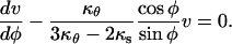
The mean cell geometry for the whole sequence was determined by fitting the curvature recorded at the fiducial points with the function where ϕ is the angle between the normal to the surface and the cell axis (Fig. 1B). This fitting function ensures that κ_s has a local minimum or maximum at ϕ = 0 and is zero at ϕ = π/2, two basic geometrical constraints for the tip geometry. The curvatures on the “right” and “left” sides of the cell were fitted independently to emphasize potential asymmetries in the cell geometry such as the slight turn for cell number 2 (Fig. 3A). The temporal variation of the geometry was quantified by calculating the mean and sd of κ_s at fixed distances from the pole (Figs. 2B and 3B).

To obtain continuous cell outlines, the fiducial points were interpolated with smoothing splines (function “csaps” in Matlab). The splines were then used to specify 1000 evenly spaced points around the cell. Figures 2A and 3A show these outlines at a 3-min time interval. The osculating circle at a given location on the cell outline was used to define the surface normal at that location. Finally, the growth axis was defined as the curve, among the family of curves orthogonal to the cell outlines, that best followed the approximate pole of the cell over the entire sequence (Figs. 2A and 3A).

The stresses acting on an axisymmetric surface loaded by internal pressure are given by the following equations (Hejnowicz et al., 1977):

(1)

(2)

where P is the turgor pressure, δ is the wall thickness, and κ_s and κ_θ are the meridional and circumferential curvatures, respectively. Since an axisymmetric dome is fully determined by one of its meridians, it is possible to write κ_θ as a function of κ_s; that is,

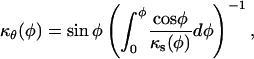where φ is a dummy variable of integration. The stresses were computed using a wall thickness (δ) of 0.1 μm (Schröter and Sievers, 1971) and a turgor pressure (P) of 0.7 MPa (Ekdahl, 1953; Lew, 1996).

Meridional Velocity and Strain Rates

For the computation of the meridional velocity, we selected microspheres that were close to the cell outline (mid-plane of the cell). Nevertheless, the displacement of some microspheres did not follow exactly the outline of the cell, indicating that the surface markers were either slightly above or below the mid-plane. Before microspheres could be used as material points, their positions had to be projected onto the cell outline (Figs. 2A and 3A). The projection was done by first finding the position of the microspheres on the first and last cell outlines, here defined as the point on these outlines closest to the first and last microsphere positions, respectively. The original microsphere trajectories were then fitted with a polynomial and “stretched” between the two new endpoints. The intersections of the new trajectories with the cell outlines were taken as the microsphere positions. For each microsphere, the meridional distance from the pole was computed and the derivative of this distance with respect to time gave the meridional velocity (Figs. 2C and 3C).

Inspection of Figures 2C and 3C reveals that the meridional velocity approximates a sine function. We can thus suggest as basic functional form to fit the velocity data the function: 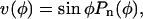where Further justification for the form of the fitting function is given in the next section. The least squares fits of the velocity data were performed for the two sides of the cell independently to reveal variations within the cell. However, two constraints had to be imposed to ensure that the resulting fits were physically sound. First, the value of c₀ on either side of the cell must be the same to yield compatible strain rates at the pole. Second, the coefficient c₁ must be zero so that the strain rates at the pole are either maxima or local minima.

To determine the appropriate degree of the polynomial P_n, we fitted the velocity data for increasing values of n. For each fit, we computed the sum of the squared residuals with the equation: 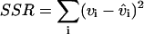where v_i is the i^th velocity measurement and is the corresponding velocity predicted by the fitting function. According to Snedecor and Cochran (1967) and Zar (1996), the significance of the reduction in SSR resulting from the addition of a new term in the fitting function can be tested with the following F-test:

(3)

where the indices r and f stand for the reduced (n − 1) and full (n) models, respectively, α is the significance level (here α = 0.01), and the degrees of freedom, df, equal the number of data points (N) minus the number of free parameters (p) in the full model. A conservative estimates of the critical F value is F_1,100,0.01 = 6.90.

For a steady rate of elongation, the strain rates can be expressed directly in terms of κ_s and v (Hejnowicz et al., 1977):

(4)

(5)

where r is the radial distance (Fig. 1B). In Equations 4 and 5, we have also used the relations and

Anisotropy Space

Three structural models are considered: isotropy, transverse isotropy, and anisotropy (Fig. 6A). To test the compatibility of these structural models with our data we need first to adopt a set of constitutive equations that relates the wall strain rates, stresses, and mechanical properties. Several constitutive models have been suggested for the plant cell wall (Lockhart, 1965a; Sellen, 1983; Chaplain and Sleeman, 1990); however, one does not need to consider these detailed models explicitly since different structural models can be formulated with simple linear constitutive relations of the form:

(6)

The matrix on the left-hand side of Equation 6 represents the wall strain rates measured in the two principal directions. The strain rates are equal to the product of a matrix of stresses (σ_i) also defined along the two principal directions and a matrix of mechanical properties (a_ij) determined by the structural model of the cell wall. The derivation of the constraints on the mechanical properties resulting from the three structural models and cell wall incompressibility is not technically demanding although somewhat cumbersome. The reader can refer to Love (1944) for such derivations. We have listed the constraints on the mechanical properties in Table II.

To illustrate how the three structural models constrain the pattern of strain rates we define two ratios: the strain rate anisotropy, 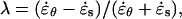and the stress anisotropy, Substituting the mechanical properties for an isotropic cell wall in Equation 6 and then substituting the strain rates into the equation for strain rate anisotropy we find the relation λ = 3γ. Therefore, for an isotropic material, the strain rate anisotropy and the stress anisotropy are proportional. Performing the same procedure for a transversely isotropic cell wall, we find the relation λ = γ(α + β)/(α − β), where α = a₁₁ = a₂₂ and β = a₁₂ = a₂₁ (note that α in this section is not the α of Eq. 3). From the constitutive relations, we can deduce that 0 ≤ β ≤ α. If β were less than zero then uniaxial tension in one direction would lead to stretching in the perpendicular direction, which is physically unrealistic. On the other hand, if β were greater than α, isotropic tension in the plane would lead to contraction instead of stretching. Given these bounds on β, the constraints on λ are: λ ≥ γ for γ > 0, λ ≤ γ for γ < 0, and λ = 0 for γ = 0. For an anisotropic model, we find that λ and γ are not constrained to specific values. These results are summarized in Table II.

The strain anisotropy and stress anisotropy reported in Figure 6B correspond to global fits of the velocity and curvature data (i.e. the left and right sides of the cell were not fitted independently). This approach was adopted because the strain anisotropy is sensitive to fluctuations when the strain rates approach zero such that small variations in the measured strain rates can lead to large variations in the calculated strain anisotropy. A global fit increases the precision of our strain measurements by including more data points into a single fit but has the disadvantage of hiding some of the variation present in the data. Therefore, the global fit was used only for illustration within Figure 6B, while the quantitative data presented in Table III were based on independent fits for the left and right sides of the cell (see below).

Model Fitting

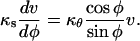
This section describes how the velocity data can be fitted such that the resulting strain rates are compatible with one of the three structural models described above. The fitting function must be such that the constitutive constraints in Table II can be enforced. We selected a fitting function based on the exact solution for an isotropic wall material. The isotropic solution can be found by substituting isotropic mechanical properties in Equation 6 (i.e. a_ss = a_θθ = 2a_sθ = 2a_θs = α). Writing Equation 6 explicitly in terms of κ_s and v, we get the following system of equations:

(7)

(8)

Dividing the first equation by the second and rearranging we get:

(9)

This differential equation for v, with boundary condition v(0) = 0, has for solution:

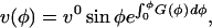(10)

where v^o is a constant, is a function of tip geometry only, and φ is a dummy variable of integration. A Taylor series expansion of the exponential term in Eq. 10 gives a polynomial in ϕ:

(11)

where a prime denotes a derivative with respect to ϕ. We are looking for a fitting function that, under its most constrained form, reduces to Equation 11 and in its most general form represents an arbitrary function. We can thus suggest as basic functional form to fit the velocity data the function:

In the solution for the isotropic model, the coefficients c_i are all determined by the derivatives of G(ϕ) at ϕ = 0 as shown in Equation 11. We note that for the isotropic model c₁ = G(0) = 0. This constraint on c₁ must always hold because it guarantees that the strain rates at the pole are maxima or local minima as required for the kinematics of tip-growing cells. If the constraints on the other coefficients of the fitting function are relaxed, more general solutions can be derived. The kinematic constraint on c₁ is indeed the only one that needs to be imposed for an anisotropic material and the resulting equation corresponds to the function used to freely fit the velocity data. To obtain solutions compatible with a transversely isotropic cell wall, a constitutive constraint must also be enforced. Inspection of Equation 6 for a transversely isotropic material reveals that and must be equal when σ_s and σ_θ are equal. If it were otherwise, no physically realistic mechanical properties would exist. From Equations 1 and 2 we observe that the stresses are equal only when the curvatures, κ_s and κ_θ, are also equal. Therefore, at the location where σ_s = σ_θ we must have and since κ_s = κ_θ, we conclude that Substitution of the fitting function in this equation gives the following constraint for a transversely isotropic material:

Finally, the three models above are compared to a reference model that has no strain anisotropy. Equating the meridional and circumferential strain rates leads to the equation:

(12)

The solution of this differential equation with boundary condition v(0) = 0 is:

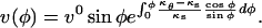(13)

A Taylor series expansion of the exponential term reduces this equation to the generic fitting function given above. The statistical analysis of the structural models used Equation 3 and the approach described above to obtain the best estimate of the strain rates.

References

- Belford DS, Preston RD (1961) The structure and growth of root hairs. J Exp Bot 12: 157–168 [Google Scholar]
- Bibikova TN, Blancaflor EB, Gilroy S (1999) Microtubules regulate tip growth and orientation in root hairs of Arabidopsis thaliana. Plant J 17: 657–665 [DOI] [PubMed] [Google Scholar]
- Castle ES (1958) The topography of tip growth in a plant cell. J Gen Physiol 41: 913–926 [DOI] [PMC free article] [PubMed] [Google Scholar]
- Chaplain MAJ, Sleeman BD (1990) An application of membrane theory to tip morphogenesis in Acetabularia. J Theor Biol 146: 177–200 [DOI] [PubMed] [Google Scholar]
- Chen JCW (1973) The kinetics of tip growth in the Nitella rhizoid. Plant Cell Physiol 14: 631–640 [Google Scholar]
- Chen JCW (1980) Longitudinal microfibrillar alignment in the wall of cylindrical Nitella rhizoidal cells: observation under polarizing and interference microscopes. Am J Bot 67: 859–865 [Google Scholar]
- Cosgrove DJ (1993) How do plant cell walls extend? Plant Physiol 102: 1–6 [DOI] [PMC free article] [PubMed] [Google Scholar]
- Ekdahl I (1953) Studies on the growth and the osmotic conditions of root hairs. Symb Bot Ups 11: 1–83 [Google Scholar]
- Green PB (1962) Mechanism for plant cellular morphogenesis. Science 138: 1404–1405 [DOI] [PubMed] [Google Scholar]
- Green PB (1963) Cell walls and the geometry of plant growth. Brookhaven Symp Biol 16: 203–217 [PubMed] [Google Scholar]
- Green PB (1965) Pathways of cellular morphogenesis. A diversity in Nitella. J Cell Biol 27: 343–363 [DOI] [PMC free article] [PubMed] [Google Scholar]
- Green PB (1973) Morphogenesis of the cell and organ axis: biophysical models. Brookhaven Symp Biol 25: 166–190 [Google Scholar]
- Green PB, King A (1966) A mechanism for the origin of specifically oriented textures in development with special reference to Nitella wall texture. Aust J Biol Sci 19: 421–437 [Google Scholar]
- Haberlandt G (1887) Über die Beziehungen zwischen Function und Lage des Zellkernes bei den Pflanzen. Fischer, Jena, Germany
- Heath IB, ed (1990) Tip Growth in Plant and Fungal Cells. Academic Press, San Diego
- Hejnowicz Z, Heinemann B, Sievers A (1977) Tip growth: patterns of growth rate and stress in the Chara rhizoid. Z Pflanzenphysiol 81: 409–424 [Google Scholar]
- Hepler PK, Vidali L, Cheung AY (2001) Polarized cell growth in higher plants. Annu Rev Cell Dev Biol 17: 159–187 [DOI] [PubMed] [Google Scholar]
- Heyn ANJ (1940) The physiology of cell elongation. Bot Rev 6: 515–574 [Google Scholar]
- Houwink AL, Roelofsen PA (1954) Fibrillar architecture of growing plant cell walls. Acta Bot Neerl 3: 385–395 [Google Scholar]
- Kataoka H (1982) Colchicine-induced expansion of Vaucheria cell apex. Alteration from isotropic to transversally anisotropic growth. Bot Mag Tokyo 95: 317–330 [Google Scholar]
- Lew RR (1996) Pressure regulation of the electrical properties of growing Arabidopsis thaliana L. root hairs. Plant Physiol 112: 1089–1100 [DOI] [PMC free article] [PubMed] [Google Scholar]
- Lloyd C (1984) Toward a dynamic helical model for the influence of microtubules on wall patterns in plants. Int Rev Cytol 86: 1–51 [Google Scholar]
- Lockhart JA (1965. a) An analysis of irreversible plant cell elongation. J Theor Biol 8: 264–275 [DOI] [PubMed] [Google Scholar]
- Lockhart JA (1965. b) Cell extension. In J Bonner, JE Varner, eds, Plant Biochemistry. Academic Press, New York
- Love AEH (1944) A Treatise on the Mathematical Theory of Elasticity. Dover, New York
- Newcomb EH, Bonnett HT (1965) Cytoplasmic microtubule and wall microfibril orientation in root hairs of radish. J Cell Biol 27: 575–589 [DOI] [PMC free article] [PubMed] [Google Scholar]
- O'Kelley JC, Carr PH (1954) An electron micrographic study of the cell walls of elongating cotton fibers, root hairs, and pollen tubes. Am J Bot 41: 261–264 [Google Scholar]
- Probine MC (1966) The structure and plastic properties of the cell wall of Nitella in relation to extension growth. Aust J Biol Sci 19: 439–457 [Google Scholar]
- Probine MC, Preston RD (1962) Cell growth and the structure and mechanical properties of the wall in internodal cells of Nitella opaca. II. Mechanical properties of the walls. J Exp Bot 13: 111–127 [Google Scholar]
- Ray PM (1987) Principles of plant cell expansion. In DJ Cosgrove, DP Knievel, eds, Physiology of Cell Expansion during Plant Growth. American Society of Plant Physiologists, Rockville, MD, pp 1–17
- Reinhardt MO (1892) Das Wachsthum der Pilzhyphen. Jahrb wiss Bot 23: 479–566 [Google Scholar]
- Richmond PA, Métraux JP, Taiz L (1980) Cell expansion patterns and directionality of wall mechanical properties in Nitella axillaris. Plant Physiol 65: 211–217 [DOI] [PMC free article] [PubMed] [Google Scholar]
- Schröter K, Sievers A (1971) Effect of turgor reduction on the Golgi apparatus and cell wall formation in root hairs. Protoplasma 22: 203–211 [Google Scholar]
- Sellen DB (1983) The response of mechanically anisotropic cylindrical cells to multiaxial stress. J Exp Bot 34: 681–687 [Google Scholar]
- Shaw SL, Dumais J, Long SR (2000) Cell surface expansion in polarly growing root hairs of Medicago truncatula. Plant Physiol 124: 959–969 [DOI] [PMC free article] [PubMed] [Google Scholar]
- Snedecor GW, Cochran WG (1967) Statistical Methods. Iowa State University Press, Ames, IA
- von Dassow M, Odell G, Mandoli D (2001) Relationships between growth, morphology and wall stress in the stalk of Acetabularia acetabulum. Planta 213: 659–666 [DOI] [PubMed] [Google Scholar]
- Wessels JGH (1986) Cell wall synthesis in apical hyphal growth. Int Rev Cytol 104: 37–79 [Google Scholar]
- Wessels JGH (1988) A steady-state model for apical wall growth in fungi. Acta Bot Neerl 37: 3–16 [Google Scholar]
- Zar JH (1996) Biostatistical Analysis. Prentice Hall, Upper Saddle River, NJ