A Robust Sparse-Modeling Framework for Estimating Schizophrenia Biomarkers from fMRI

Abstract

Background

Our goal is to identify the brain regions most relevant to mental illness using neuroimaging. State of the art machine learning methods commonly suffer from repeatability difficulties in this application, particularly when using large and heterogeneous populations for samples.

New Method

We revisit both dimensionality reduction and sparse modeling, and recast them in a common optimization-based framework. This allows us to combine the benefits of both types of methods in an approach which we call unambiguous components. We use this to estimate the image component with a constrained variability, which is best correlated with the unknown disease mechanism.

Results

We apply the method to the estimation of neuroimaging biomarkers for schizophrenia, using task fMRI data from a large multi-site study. The proposed approach yields an improvement in both robustness of the estimate and classification accuracy.

Comparison with Existing Methods

We find that unambiguous components incorporate roughly two thirds of the same brain regions as sparsity-based methods LASSO and elastic net, while roughly one third of the selected regions differ. Further, unambiguous components achieve superior classification accuracy in differentiating cases from controls.

Conclusions

Unambiguous components provide a robust way to estimate important regions of imaging data.

1. Introduction

In this paper our goal is to find the most relevant brain regions given labeled neuroimaging data; the ultimate goal is to use those results to understand disease mechanisms, as well as to provide biomarkers to help diagnose (i.e., classify) patients as having disease or not. There is a significant need for techniques which can robustly extract information in such a problem. Neuroimaging, particularly functional neuroimaging, has provided a wealth of intriguing information regarding brain function, but has yet to show clear value to psychiatric diagnosis [19]. Despite this, impressive results have been achieved with machine learning techniques such as support vector machines, which demonstrate high classification accuracies [24]. Reproducibility problems persist however [5], with an apparent trend towards poorer performance for larger studies [27].

The identification of meaningful components of the data is a key benefit of many feature selection techniques [17], in addition to providing improvements in performance of subsequent classification stages [9]. In a typical neuroimaging study there may be tens or hundreds of subjects, each with an image consisting of up to hundreds of thousands of voxels, resulting in an extremely underdetermined problem. A popular category of feature selection approaches is regularized regression techniques such as LASSO [29] and related methods employing sparse models [6, 21]. Such supervised techniques impose task-specific information (the data labels), with a penalty term to incorporate prior knowledge. In the case of LASSO, the prior knowledge amounts to a presumption of sparsity on the relationship between image data and labels, i.e., that the underlying biological mechanism involves a limited number of the imaged voxels. Unfortunately, if the problem is both very underdetermined and very noisy, then the regularized solution may not be a particularly superior choice; many solutions may potentially be of similar or even equal probability to each other. For example in the underdetermined case, the LASSO solution may not be unique for highly-structured datasets [30, 33]. Along these lines, we simply may not have sufficient confidence in the validity of our prior knowledge formulation to presume that the most regular solution is preferable to those even moderately as regular.

From a different direction, dimensionality reduction techniques [20] offer a more robust approach to feature selection in neuroimaging data. An example is principal component analysis (PCA) [13], which finds basis vectors for the space containing the data variation. This set of basis vectors can be viewed as robust in the sense that they are common to all solutions of any linear regression based on the data. In statistics a closely-related concept is estimable functions [23]. We will refer to components with such a property as unambiguous, and examine this more formally in the next section. Of course such components only describe the data itself, not necessarily the aspects of the data pertinent to our application, such as for finding information most related to a disease phenotype. A common approach is to utilize PCA and related factoring methods in a supervised fashion by choosing a subset of factors which best correlate with the labels. Supervised factoring techniques such as the “Supervised PCA” of [3], and related methods, can be viewed as a more sophisticated version of this technique, finding a transformation of the data such that the correlation with the labels is maximized. However these techniques are not able to incorporate prior knowledge, such as sparsity of the mechanism, into this transformation. Techniques have been developed which do incorporate sparsity into unsupervised factoring techniques (e.g., sparse PCA [35]) in a heuristic sense, though this differs from presuming sparsity of the underlying mechanism; the presumption of sparsity is applied to the structure of the component itself rather than to the unknown mechanism. Hybrid methods have been proposed which perform PCA following a pre-screening step which picks a subset of variables over a correlation threshold [2] or in known pathways [22]. However we would prefer to incorporate multi-variable relationships in the screening component.

In this paper, we develop an approach which combines the benefits of both regularized estimates and dimensionality reduction by simultaneously enforcing unambiguity and prior knowledge in calculating components. We start by reviewing dimensionality reduction from the perspective of unambiguous components. Then we review related regularization methods and show how they motivate our approach to incorporate prior knowledge into unambiguous components. By maximizing the correlation with the mechanism, we calculate components which identify the most important regions in the data. We use a simulation to show how this component performs robustly in the face of inaccurate prior knowledge, by demonstrating that the correlation still remains controlled as the prior knowledge is relaxed. Finally, we show a successful application to biomarker identification where we identify features of fMRI data which relate to schizophrenia more accurately than other methods which utilize sparsity as prior knowledge.

2. Materials and Methods

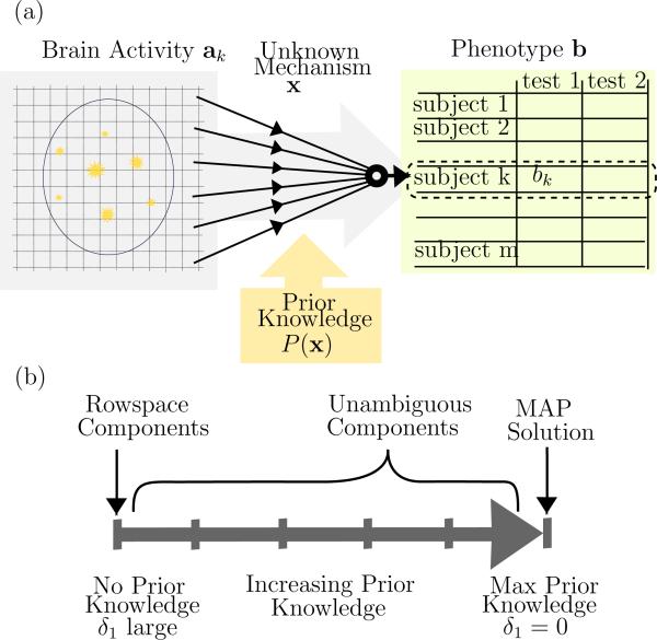
We will consider the linear model Ax = b+n where A is a m×n data matrix with n > m, containing samples as rows, and variables as columns; b is the phenotype encoded into a vector of labels such as case or control; the solution x is the unknown model parameters that relate A to b ; and n is a noise vector about which we have only statistical information. We will also assume the means have been removed from b and the columns of A to simplify the presentation. The rows of A are provided by the contrast images from individual study subjects, so a predictor x selects a weighted combination of voxels (i.e., columns of A) which relates the imagery to the case-control status. By examining the weightings in this combination we hope to learn more about the spatial distribution of causes or effects of the disease, which we will term the “mechanism” in this paper. The model is depicted in Fig. 1 (a), where we depict the true solution x as the mechanism whereby brain activity relates to the measured phenotypes. Of course there are far more unknown variables than samples, hence our linear system is underdetermined and there will be many possible x which solve the system. One way to address this problem is to impose prior knowledge about the biological mechanism, such as a preference for sparser x, and select the solution which best fulfills this preference. We will review this approach in a later section. Another approach is to restrict our analysis to components of the solution which may be more easily estimated, such as via dimensionality reduction; an intuitive example of this approach is to group voxels into low-resolution regions. These alternatives are depicted in Fig. 1 (b), as extremes on a continuum of possible methods, where the goal of this paper is to find intermediate information which utilizes the benefits of both extremes.

Figure 1.

(a) Mathematical model Ax = b, where x describes the mechanism that relates brain activity to phenotype (psychiatric assessments). The contrast map for a single subject, a_k, provides the kth row of A. As there are still many unknown biological variables, the problem is underdetermined and x cannot be found uniquely; instead we must settle for a probable result such as a maximum likelihood solution which utilizes prior knowledge, or an estimable component of x. (b) Continuum between rowspace components and most probable solution, based on increasing confidence in the prior knowledge, which we control by the relaxation parameter δ₁.

2.1. Dimensionality Reduction

To see how dimensionality reduction can apply to the estimation of mechanism, consider the Singular Value Decomposition (SVD) of A = USV^T, where S is a diagonal matrix of singular values σ_i, and U and V contain the left and right singular vectors u_i and v_i. In Principal Components Analysis (PCA) the focus is on this expansion itself, however our focus here is on the mechanism which we model by x. If we plug USV^T into Ax = b and apply the transformation U^T to both sides, we get a diagonalized system with decoupled equations of the form ${\sigma }_i{\mathbf{v}}_i^T\mathbf{x}={\mathbf{u}}_i^T\mathbf{b}$. This equation tell us that, while we can't calculate the true x in the underdetermined case, we can calculate components of x corresponding to nonzero singular values. One way to view this property is by considering that these components are constant for all possible x given our linear system. In other words, ${\sigma }_i{\mathbf{v}}_i^T\mathbf{x}$ calculates the same value for any solution in the set {x | Ax = b}. In terms of our application, this means while we can't identify the true mechanism x, we can extract reliable components of it. For example, we might be able to coarsely identify large regions containing important activity, without being able to pinpoint particular voxels within those regions. Of course the SVD selects vectors based on orthogonal directions of ranked data variation, which may not be best suited to provide information about the disease mechanism. We will address this later by optimizing the choice of component, but first we will formally consider this property of constant components so that we may extend it later to incorporate prior knowledge.

2.2. Unambiguous Components without Prior Knowledge

In this section we will introduce the idea of unambiguous components in the noise-free case without prior knowledge. The concept is demonstrated geometrically in Fig. 2 (a), where the useful information in A forms the matrix rowspace; this contains the dimensions over which we have a diversity of data which we can compare to the phenotype b. Dimensions perpendicular to the rowspace form the nullspace, directions over which our data does not vary. For example if our dataset was composed of subjects with the same age, then we cannot perform a regression to see how disease risk relates to age. In terms of components of the data, if c is a loading vector and a_i is a sample (row of A), then c^Ta_i is potentially useful information when c is in the rowspace, and useless information (in fact always zero) when c is in the nullspace. An equivalent perspective, depicted in Fig. 2 (b), is the geometry of the solution set to the regression model. This is the affine set S_EC, composed of an offset (the least-length solution x₀) plus a vector from the nullspace.

$$S_{EC}=\{\mathbf{x}\mid \mathbf{Ax}=\mathbf{b}\}.$$ (1)

The subscript “EC” refers to x being only equality-constrained (i.e., we have imposed no prior knowledge yet). The rowspace vectors yield estimable components of x given the data, while nullspace vectors give the dimensions of ambiguity we have about x. We will formulate this relationship rigorously next.

Figure 2.

Two-dimensional example: (a) The rowspace of A is the direction of data diversity, while the nullspace is perpendicular directions, which lack diversity. (b) The solution set to Ax = b is the affine space S_EC, which is parallel to the nullspace; the ambiguity due to lack of data diversity results in ambiguity of possible solutions forming S_EC. (c) The distribution of x resulting from the likelihood P(b|x), the high probability region is nearest S_EC. (d) The set S_DR formed by the intersection of a bound on P(b|x) enforced by ∥Ax – b∥₂ ≤ α₂, and a bound on the prior distribution P(x) enforced by ∥x∥₁ ≤ α₁; the LASSO solution x₁ is based on a trade-off where the combination of bounds must be as tight as possible.

Recall that the rowspace of A is defined as the set of all possible linear combinations of rows, i.e., $\mathcal{R}\left({\mathbf{A}}^T\right)=\{\mathbf{c}\mid {\mathbf{A}}^T\mathbf{y}=\mathbf{c}\forall \mathbf{y}\in {\mathbb{R}}^m\}$. We can equivalently view this as a set whose members take on a constant value over S_EC. In other words, they form the set of unambiguous components for S_EC. We state this simple but important fact in Theorem 1.

Theorem 1

The following two statements are equivalent:

1. $\mathbf{c}\in \mathcal{R}\left({\mathbf{A}}^T\right)$.

2. c^Tx = μ for all x ∈ S_EC, where μ is a constant.

Proof

It is straightforward to note that, as A^Ty = c, we have c^Tx = y^TAx = y^Tb ≡ μ. However it will be useful to our subsequent extension to note the fact that the rows-pace is the orthogonal complement to the nullspace, and can be also written as $\mathcal{R}\left({\mathbf{A}}^T\right)=\{\mathbf{c}\mid {\mathbf{c}}^T\mathbf{z}=0\forall \mathbf{z}\in \mathcal{N}\left(\mathbf{A}\right)\}$. Equivalently, any vector z in the nullspace may be described as a difference between solutions, i.e., z = x₁ – x₂, where x₁, x₂ ∈ S_EC. Therefore the rowspace may also be written as $\mathcal{R}\left({\mathbf{A}}^T\right)=\{\mathbf{c}\mid {\mathbf{c}}^T{\mathbf{x}}_1={\mathbf{c}}^T{\mathbf{x}}_2\forall {\mathbf{x}}_1,{\mathbf{x}}_2\in S_{EC}\}$, which explicitly states the equivalence in Theorem 1.

The principal components of A corresponding to the r nonzero singular values must be in the rowspace. Again, given a singular-value decomposition A = USV^T, we have VSU^Ty = c for $\mathbf{c}\in \mathcal{R}\left({\mathbf{A}}^T\right)$, and hence ${\mathbf{V}}^T\mathbf{c}={\mathbf{SU}}^T\mathbf{y}={\sum }_{i=1}^r{\sigma }_i{\mathbf{u}}_i$, where the u_i for i ∈ {1, ..., r} form a basis for the rowspace. So principal components are unambiguous components.

Later we will also consider how to optimize the choice of component such that it also computes a score which is maximally useful for an application (such as to identify important image regions for classification of disease). But first we will extend the concept of unambiguous components to incorporate prior knowledge. Our focus on components of the mechanism x rather than of the data a_i allows us to incorporate prior knowledge which applies to x into the method, such as the presumption of a sparse biological mechanism. In effect, we will utilize prior knowledge to further restrict the variation in x and potentially increase the estimable components of x.

2.3. LASSO and Elastic Net

In this section we will review closely-related estimation methods which utilize prior knowledge, to provide an intuitive basis for our mathematical formulation. The Maximum A Posteriori (MAP) estimate x_MAP is the solution which maximizes the posterior probability P(x|b) over x. Using Bayes’ theorem, we can form the equivalent problem, arg max_x P(b|x)P(x), which utilizes the likelihood P(b|x) (essentially the distribution for n), and the prior probability distribution P(x). It is the form of this prior distribution which we refer to as the prior knowledge. A common approach is to take the log of this objective to get a penalized regression problem. With a Gaussian distribution for n and a Laplace distribution for x, taking the log yields the most well-known version of LASSO, ${\min }_{\mathbf{x}}{\Vert \mathbf{Ax}-\mathbf{b}\Vert }_2^2+\lambda {\Vert \mathbf{x}\Vert }_1$. LASSO was originally proposed in the form, ${\min }_{\mathbf{x}}{\Vert Ax-\mathbf{b}\Vert }_2^2$ subject to ${\Vert \mathbf{x}\Vert }_1\le {\alpha }_1$, with the other version sometimes described as the Lagrangian form. It can be shown that for any λ, a α₁ exists such that these optimization problems have the same minimizer, x₁. We can similarly form the feasibility problem (an optimization problem which stops when any feasible point is found, hence we simply use a zero for the objective as it is irrelevant [4]),

$$\begin{array}{cc}\hfill {\mathbf{x}}_1=\hfill & \hfill \arg \underset{\mathbf{x}}{\min }0\hfill \\ \hfill \hfill & \hfill {\Vert \mathbf{x}\Vert }_1\le {\alpha }_1\hfill \\ \hfill \hfill & \hfill {\Vert Ax-\mathbf{b}\Vert }_2\le {\alpha }_2\hfill \end{array}$$ (2)

In this paper we will focus on sets of the general form of this feasible set we will denote as S_DR. In terms of the statistical distributions, the constraints on the norms amount to constraints on the probabilities, as in

$$S_{DR}=\{\mathbf{x}\mid {\Vert \mathbf{x}\Vert }_1\le {\alpha }_1,{\Vert \mathbf{Ax}-\mathbf{b}\Vert }_2\le {\alpha }_2\}.$$ (3)

$$=\{\mathbf{x}\mid P\left(\mathbf{x}\right)\ge P_{min},P(\mathbf{Ax}-\mathbf{b})\ge P_{min}\}.$$ (4)

The subscript DR refers to the combination of denoising and regularization constraints. It can also be shown that x₁ which solves the previous versions, will provide a member of this set. Therefore, we may write the LASSO problem as

$$\begin{array}{cc}\hfill {\mathbf{x}}_1=\hfill & \hfill \arg \underset{\mathbf{x}}{\min }0\hfill \\ \hfill \hfill & \hfill \mathbf{x}\in S_{DR}\hfill \end{array}$$ (5)

The elastic net [34] can be viewed as a variation on LASSO, where (under the Bayesian framework) the Laplace prior distribution for the prior is replaced by a product of Laplace and Gaussian distributions. Taking the log of the posterior distribution leads to the well-known problem ${\min }_{\mathbf{x}}{\Vert \mathbf{Ax}-\mathbf{b}\Vert }_2^2+{\lambda }_1{\Vert \mathbf{x}\Vert }_1+{\lambda }_2{\Vert \mathbf{x}\Vert }_2^2$. As with LASSO, we may achieve the same solution using different optimization problems. We wish to use the same constraints as earlier, so we form the related problem,

$$\begin{array}{ccc}\hfill {\mathbf{x}}_2=\hfill & \hfill \arg \underset{\mathbf{x}}{\min }{\Vert \mathbf{x}\Vert }_2^2\hfill & \hfill =\arg \underset{\mathbf{x}}{\min }{\Vert \mathbf{x}\Vert }_2^2\hfill \\ \hfill \hfill & \hfill {\Vert \mathbf{x}\Vert }_1\le {\alpha }_1\hfill & \hfill \mathbf{x}\in S_{DR}.\hfill \\ \hfill \hfill & \hfill {\Vert \mathbf{Ax}-\mathbf{b}\Vert }_2\le {\alpha }_2\hfill & \hfill \hfill \end{array}$$ (6)

Recall that LASSO seeks any single solution within S_DR. In that case, α₁ and α₂ are chosen as small as possible so the set is (hopefully) a singleton. Elastic net, on the other hand, seeks the least length solution in S_DR, where we may choose α₁ and α₂ more loosely, to trade-off desirable properties of this solution. These are depicted in Fig. 2 (d), where the LASSO solution, x₁ is formed by tightening the bounds on the two sets (one representing the prior and one representing the noise) to minimal intersection. The elastic net solution, by contrast, relaxes the constraints on the two sets forming the larger set S_DR, and selection of the least length solution in this intersection. Next we will extend the unambiguous component idea to utilize S_DR, thereby incorporating prior knowledge into the framework.

Finally, note that the norms ∥ · ∥₁ and ∥ · ∥₂ may be replaced with other choices of norms representing other forms of prior knowledge, such as the ℓ_∞-norm, which imposes hard limits on the unknowns or the error, and which might result from box constraints [1] or a minimax regression [26]. More complex forms of penalties are used in the elastic net [34], and methods utilizing mixed norms [18] such as group LASSO [32]. The methods and theoretical results in this paper are generally the same as long as the choice fulfills the mathematical properties of a norm (though this is not a strict requirement).

2.4. Unambiguous Components Subject to Prior Knowledge

Earlier, we introduced unambiguous components as components of the unknown solution, which computed a constant score over all possible solutions. Now we will extend this concept to replace the set of possible solutions (S_EC) with a set of highly-probable solutions, for which we will use S_DR. We will also extend the requirement that the score be constant to a requirement that their variation is limited within a fixed bound. So in effect, given a pool of solutions, which we may view as the most likely hypotheses for the underlying mechanism, we will seek components which compute approximately-constant scores for every likely mechanism.

We incorporate prior knowledge as well as bounds on the score by relaxing the rowspace with the following generalization,

$$R_S\left(ϵ\right)=\{\mathbf{c}\mid \mid {\mathbf{c}}^T{\mathbf{x}}_1-{\mathbf{c}}^T{\mathbf{x}}_2\mid \le ϵ\forall {\mathbf{x}}_1,{\mathbf{x}}_2\in S_{DR}\}$$ (7)

$$=\{\mathbf{c}\mid {\mathbf{c}}^T{\mathbf{x}}_1-{\mathbf{c}}^T{\mathbf{x}}_2\le ϵ\forall {\mathbf{x}}_1,{\mathbf{x}}_2\in S_{DR}\}.$$ (8)

Here we have relaxed the ambiguity to potentially allow a positive bound ϵ, as well as replaced S_EC with S_DR. Note that we were able to remove the absolute value in Eq. (8) because membership in R_S(ϵ) requires the inequality hold for all x₁, x₂ ∈ S_DR, hence if it holds for ${\mathbf{x}}_1^{\prime }$, ${\mathbf{x}}_2^{\prime }$, it must also hold for ${\mathbf{x}}_1^{″}$, ${\mathbf{x}}_2^{″}$ where ${\mathbf{x}}_1^{″}={\mathbf{x}}_2^{\prime }$ and ${\mathbf{x}}_2^{″}={\mathbf{x}}_1^{\prime }$. To highlight the view of this set as a generalization of the rowspace, we state the following simple generalization of Theorem 1, without proof,

Theorem 2

The following two statements are equivalent:

1. c ∈ R_S(ϵ)

2. $\mu -\frac{1}{2}ϵ\le {\mathbf{c}}^T\mathbf{x}\le \mu +\frac{1}{2}ϵ$ for all x ∈ S_DR, where μ is a constant.

Note that while this formulation appears quite simple, it will generally not be possible to describe R_S(ϵ) in a closed form or analytically determine whether a vector is a member of R_S(ϵ). However we may use convex optimization theory to formulate R_S(ϵ) as a system of inequalities. We defined R_S(ϵ) via the test c^Tx₁ – c^Tx₂ ≤ ϵ, which may also be written as c^T(x₁ – x₂) ≤ ϵ. We may use optimization to directly perform this test as follows,

$$\begin{array}{cc}\hfill p=\hfill & \hfill \underset{\mathbf{x},{\mathbf{x}}^{\prime }}{\max }{\mathbf{c}}^T(\mathbf{x}-{\mathbf{x}}^{\prime })\hfill \\ \hfill \hfill & \hfill \mathbf{x}\in S_{DR}\hfill \\ \hfill \hfill & \hfill {\mathbf{x}}^{\prime }\in S_{DR}.\hfill \end{array}$$ (9)

If the optimal value p ≤ ϵ, then we were unable to find any pair of solutions to demonstrate an ambiguity in the component score greater than ϵ, and hence c ∈ R_s(ϵ). Similar methods have been proposed elsewhere to use optimization to test boundedness [10] and uniqueness [11, 30] of solutions to systems with particular forms of prior knowledge; in those cases the test was performed over individual variables, whereas we will use a test for a general component c here. S_DR is a convex set so this is a straightforward convex optimization problem for either maximization or minimization, and so we can be assured of finding a global optima with an efficient algorithm [4]. If we replace S_DR with S_EC we have the equality-constrained linear program [14],

$$\begin{array}{cc}\hfill p=\hfill & \hfill \underset{\mathbf{x},{\mathbf{x}}^{\prime }}{\max }{\mathbf{c}}^T(\mathbf{x}-{\mathbf{x}}^{\prime })\hfill \\ \hfill \hfill & \hfill \mathbf{Ax}=\mathbf{b}\hfill \\ \hfill \hfill & \hfill {\mathbf{Ax}}^{\prime }=\mathbf{b}.\hfill \end{array}$$ (10)

Unless c is in the rowspace of A, this optimization problem will be unbounded. So the optimality condition for Eq. (10) is the now-familiar requirement that a solution can be found to A^Ty = c.

It is not useful to relax the ambiguity in the equality-constrained case (there, p is either zero or infinite), but for S_DR we can form general conditions for c ∈ R_S(ϵ) incorporating a relaxed upper limit p ≤ ϵ. The analogous set of conditions achieved using S_DR instead of S_EC, and allowing a non-zero ϵ, is the following, as we will show with Theorem 3,

$$\begin{array}{c}\hfill {\mathbf{b}}^T(\mathbf{y}+{\mathbf{y}}^{\prime })+{\alpha }_1({\lambda }_1+{\lambda }_1^{\prime })+{\alpha }_2({\lambda }_2+{\lambda }_2^{\prime })\le ϵ\hfill \\ \hfill {\Vert {\mathbf{A}}^T\mathbf{y}-\mathbf{c}\Vert }_{\infty }\le {\lambda }_1\hfill \\ \hfill {\Vert {\mathbf{A}}^T{\mathbf{y}}^{\prime }+\mathbf{c}\Vert }_{\infty }\le {\lambda }_1^{\prime }\hfill \\ \hfill {\Vert \mathbf{y}\Vert }_2\le {\lambda }_2\hfill \\ \hfill {\Vert {\mathbf{y}}^{\prime }\Vert }_2\le {\lambda }_2^{\prime }.\hfill \end{array}$$ (11)

This is the generalization of the rowspace condition A^Ty = c to R_S(ϵ). We show this with the following theorem,

Theorem 3

If there exists a y, y′, λ₁ ${\lambda }_1^{\prime }$, λ₂ and ${\lambda }_2^{\prime }$ such that c is a solution to Eqs. (11), then c ∈ R_s(ϵ).

Proof

We can test the limits of c^Tx with the optimization problem of Eq. (9) with S = S_DR,

$$\begin{array}{cc}\hfill p=\hfill & \hfill \underset{\mathbf{x},{\mathbf{x}}^{\prime }}{\max }{\mathbf{c}}^T(\mathbf{x}-{\mathbf{x}}^{\prime })\hfill \\ \hfill \hfill & \hfill {\Vert \mathbf{x}\Vert }_1\le {\alpha }_1\hfill \\ \hfill \hfill & \hfill {\Vert {\mathbf{x}}^{\prime }\Vert }_1\le {\alpha }_1\hfill \\ \hfill \hfill & \hfill {\Vert \mathbf{Ax}-\mathbf{b}\Vert }_2\le {\alpha }_2\hfill \\ \hfill \hfill & \hfill {\Vert {\mathbf{Ax}}^{\prime }-\mathbf{b}\Vert }_2\le {\alpha }_2.\hfill \end{array}$$ (12)

By forming the dual [4] of the optimization problem in Eq. (12), we can get an upper bound on the optimal. The dual optimization problem is

$$\begin{array}{cc}\hfill d=\hfill & \hfill \underset{\begin{array}{c}\hfill \mathbf{y},{\mathbf{y}}^{\prime },\hfill \\ \hfill {\lambda }_1,{\lambda }_1^{\prime },\lambda ,{\lambda }^{\prime }\hfill \end{array}}{\min }\{{\mathbf{b}}^T(\mathbf{y}+{\mathbf{y}}^{\prime })+{\alpha }_1({\lambda }_1+{\lambda }_1^{\prime })+{\alpha }_2(\lambda +{\lambda }^{\prime })\}\hfill \\ \hfill \hfill & \hfill {\Vert {\mathbf{A}}^T\mathbf{y}-\mathbf{c}\Vert }_1^{\ast }\le {\lambda }_1\hfill \\ \hfill \hfill & \hfill {\Vert {\mathbf{A}}^T{\mathbf{y}}^{\prime }+\mathbf{c}\Vert }_1^{\ast }\le {\lambda }_1^{\prime }\hfill \\ \hfill \hfill & \hfill {\Vert \mathbf{y}\Vert }_2^{\ast }\le {\lambda }_2\hfill \\ \hfill \hfill & \hfill {\Vert {\mathbf{y}}^{\prime }\Vert }_2^{\ast }\le {\lambda }_2^{\prime },\hfill \end{array}$$ (13)

where ∥ · ∥* is the dual norm of ∥ · ∥. For example the dual norm for the ℓ₁-norm is the ℓ_∞-norm (we provide this general result to allow for other choices of norms if desired). The weak duality condition [4], which always holds, tells us that p ≤ d. By constraining the objective of Eq. (13) to be bounded by ϵ, which would mean c ∈ R_S(ϵ), we get the conditions of Eqs. (11).

Note that strong duality holds for convex optimization problems as well as many non-convex problems under a broad set of conditions, the most well-known being Slater's condition [4]. When strong duality holds, the converse of Theorem 3 holds as well, and so our conditions hold for all elements of R_S(ϵ). We will presume this is the case. Next we will consider the choice of useful components which fulfill the conditions of Eqs. (11).

2.5. Optimizing Components

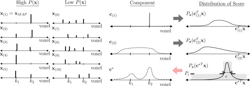
The motivation and strategy of our approach are summarized in Fig. 3. For a hypothetical example, we give several potential solutions to Ax = b which we denote as x_(i), where Ax_(i) = b for all i. Recall each solution is a potential mechanism. For example, potential solution x₍₁₎ suggests the mechanism is based on activity at voxel k₂, while potential solution x₍₄₎ suggests the mechanism is based on activity at voxel k₁. Choosing any single solution such as the MAP solution is risky as it may lead us to the wrong voxel if incorrect. We can analyze the risk of a choice of solution by looking at its correlation with other high-probability solutions. If we treat the choice of solution as an alternative candidate for a component, we may equivalently evaluate this risk by examining the marginal distribution of the score computed by this component. In Fig. 3 we depict multiple options for components; c₍₁₎ is the MAP solution, while c₍₂₎ calculates the an average over a large region. Fig. 3 also gives the distributions for the scores computed by these components (i.e., the range of correlations with potential solutions), where we see that these two result in broad distributions. Such broad distributions imply a wide possible variation in correlation with the different possible solutions, meaning these components are not very unambiguous, and hence are poor representatives of the set of high-probability solutions. Our strategy is depicted in Fig. 3 by the distribution for P(c*^Tx), where we set desired limits on the spread of the correlations, and use optimization to choose an optimal c* which fulfills these requirements. We can implement this strategy, therefore, using the conditions we derived in the previous section, recalling the relationship between the constraint sets and the distributions of Eq. (4).

Figure 3.

Example giving several solutions x with higher and lower P(x), candidate components, and the marginal probability distribution of feature values; The broader the spread of the values for a given feature, the more ambiguous the feature. The design problem of calculating c based on constraints ϵ and P_ϵ (which is based on α₁ and α₂), amounts to finding a component who's value has a controlled statistical spread.

Further, in order to choose the unambiguous component which is most useful for identifying properties of the mechanism, not only do we seek a component which is unambiguous, we also wish for the correlation with potential solutions to be maximized. To motivate this approach, consider the following robust strategy. Suppose instead of seeking an unambiguous component, we simply sought a component which had high correlations with all possible x ∈ S_DR using the following minimax strategy,

$${\mathbf{x}}^{\ast }=\arg \underset{\Vert \mathbf{c}\Vert =1}{\max }\underset{\mathbf{x}\in S_{DR}}{\min }{\mathbf{c}}^T\mathbf{x}$$ (14)

Here we seek the c for which the worst-possible correlation with high-probability solutions x ∈ S_DR is maximized. If we exchange the maximization and minimization to get min_xϵSDRmax_∥c∥=1 c^Tx, then we can analytically solve the inner maximization to get min_x∈SDR∥x∥₂, which is a variation on the elastic net of Eq. (6). So the elastic net can be viewed as a robust strategy to choose a vector c which maximizes the worst-case correlation with possible mechanisms, defined by S_DR.

For an unambiguous component, the correlations c^Tx will be approximately equal for all x ∈ S_DR by design. Therefore, we can simply choose an unambiguous component with maximum correlation using the following optimization (which we will call the UMAX problem, for Unambiguous Maximum correlation),

$$\begin{array}{cc}\hfill {\mathbf{c}}_{UMAX}=\hfill & \hfill \arg \underset{\mathbf{c},\mathbf{x}}{\max }{\mathbf{c}}^T\widehat{\mathbf{x}}\hfill \\ \hfill \hfill & \hfill \mathbf{c}\in R_S\hfill \\ \hfill \hfill & \hfill \Vert \mathbf{c}\Vert \le 1.\hfill \end{array}$$ (15)

where x̂ is any solution in S_DR, such as the LASSO solution x₁. We also relaxed the unit length constraint to an inequality constraint ∥c∥ ≤ 1, making the optimization convex. In the extreme case where S_DR is small and only contains close approximations to x₁, the optimal c will converge to x₁.

Optimization also provides an opportunity to impose additional properties on the component vector c. In particular, we may independently impose sparsity of our component (not to be confused with the sparsity prior which applies to the mechanism). In Eq. (16), we trade o a degree of sparsity on c and correlation with the mechanism, based on a choice of regularization parameter η.

$$\begin{array}{cc}\hfill {\mathbf{c}}_{\eta }=\hfill & \hfill \arg \underset{\begin{array}{c}\hfill \mathbf{c},\mathbf{y},{\mathbf{y}}^{\prime },\hfill \\ \hfill {\lambda }_1,{\lambda }_1^{\prime },{\lambda }_2,{\lambda }_2^{\prime }\hfill \end{array}}{\max }\{{\mathbf{c}}^T{\mathbf{x}}_0-\eta {\Vert \mathbf{c}\Vert }_1\}\hfill \\ \hfill \hfill & \hfill {\mathbf{b}}^T(\mathbf{y}+{\mathbf{y}}^{\prime })+{\alpha }_1({\lambda }_1+{\lambda }_1^{\prime })+{\alpha }_2({\lambda }_2+{\lambda }_2^{\prime })\le ϵ\hfill \\ \hfill \hfill & \hfill {\Vert {\mathbf{A}}^T\mathbf{y}-\mathbf{c}\Vert }_{\infty }\le {\lambda }_1\hfill \\ \hfill \hfill & \hfill {\Vert {\mathbf{A}}^T{\mathbf{y}}^{\prime }+\mathbf{c}\Vert }_{\infty }\le {\lambda }_1^{\prime }\hfill \\ \hfill \hfill & \hfill {\Vert \mathbf{y}\Vert }_2\le {\lambda }_2\hfill \\ \hfill \hfill & \hfill {\Vert {\mathbf{y}}^{\prime }\Vert }_2\le {\lambda }_2^{\prime }\hfill \\ \hfill \hfill & \hfill {\Vert \mathbf{c}\Vert }_2\le 1.\hfill \end{array}$$ (16)

For comparison, the following provides a similar optimization without the imposition of prior knowledge,

$$\begin{array}{cc}\hfill {\mathbf{c}}_{EC}^{\ast }=\hfill & \hfill \arg \underset{\mathbf{c},\mathbf{y}}{\max }\{{\mathbf{c}}^T{\mathbf{x}}_0-\eta {\Vert \mathbf{c}\Vert }_1\}\hfill \\ \hfill \hfill & \hfill {\mathbf{A}}^T\mathbf{y}=\mathbf{c}\hfill \\ \hfill \hfill & \hfill {\Vert \mathbf{c}\Vert }_2\le 1.\hfill \end{array}$$ (17)

This component is simply the best choice according to our heuristic which can be found within the rowspace. Techniques which select combinations of principal components such as sparse PCA or supervised PCA, essentially form a variation of Eq. (17).

3. Results

In this section we will demonstrate the method, first with simulations which illustrate the ability to control the variance of the component, then with real data where we compare the method to LASSO and elastic net for feature selection.

3.1. Simulation

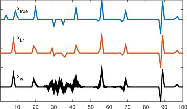
First, we performed a simulation which demonstrated the robustness of the unambiguous component (i.e., the limited spread of its correlation with all other potential mechanisms). For this example, the minimum ℓ₁-norm (Basis Pursuit [8]) solution is itself not unique. To explore this, we use this solution set as S_DR, so α₂ = 0, and α₁ computed from the Basis Pursuit solution, α₁ = min_x ∥x∥₁ subject to Ax = b. The matrix A is 20 × 100 with binary random elements A_ij ∈ {−1, +1}. Such highly-structured matrices often fail to yield unique solutions for ℓ₁-norm based techniques [12]. The true solution x_true is a sparse vector, plotted in Fig. 4, and b = Ax_true. Fig. 4 also gives the Basis Pursuit solution, and a variety of other solutions that have the same ℓ₁-norm (computed randomly), to demonstrate the non-uniqueness of the Basis Pursuit solution for this system.

Figure 4.

True x, Basis Pursuit solution (x_L1), and various other randomly-found solutions (x_w) plotted on top of each other, where ∥x_L1∥₁ = ∥x_w∥₁.

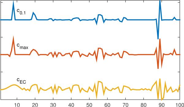
In Fig. 5 we give the components computed via Eq. (16) with η = 0.1 (c_0.1) and with η = 0(c_max). We used ϵ = 0.01 to allow for finite numerical precision. We also computed the analogous maximum component in the rowspace, c_EC, using η = 0 in Eq. (17).

Figure 5.

Different candidates for computing feature.

To demonstrate the robust behavior of the components, we used the optimization approach of Eq. (12) to measure the range of values each component c^Tx could take. We repeated this optimization over a range of relaxations of the prior knowledge, where we replaced α₁ with α₁ + δ₁ as in the following,

$$\begin{array}{cc}\hfill p\left({\delta }_1\right)=\hfill & \hfill \underset{\mathbf{x},{\mathbf{x}}^{\prime }}{\max }{\mathbf{c}}^T(\mathbf{x}-{\mathbf{x}}^{\prime })\hfill \\ \hfill \hfill & \hfill {\Vert \mathbf{x}\Vert }_1\le {\alpha }_1+{\delta }_1\hfill \\ \hfill \hfill & \hfill {\Vert {\mathbf{x}}^{\prime }\Vert }_1\le {\alpha }_1+{\delta }_1\hfill \\ \hfill \hfill & \hfill {\Vert \mathbf{Ax}-\mathbf{b}\Vert }_2\le {\alpha }_2\hfill \\ \hfill \hfill & \hfill {\Vert {Ax}^{\prime }-\mathbf{b}\Vert }_2\le {\alpha }_2.\hfill \end{array}$$ (18)

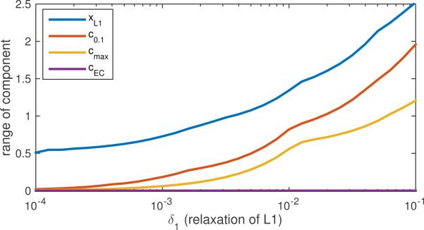
So when δ₁ = 0, we have a test of the correlations with all possible solutions that have the same ℓ₁-norm as the Basis Pursuit solution. In Fig. 6 we see that the unambiguous components we computed achieve p ≤ 0.01 for δ₁ → 0, as they were designed to, and as does the rowspace solution c_EC. Once this prior knowledge is relaxed by increasing δ₁, however, c_max and c_0.1 cease to yield unique values for c^Tx. For comparison we also demonstrate the correlation with the Basis Pursuit solution itself, x_L1. We see that it always results in a higher range p for the ambiguity, which demonstrates that x_L1 is a poorer choice for a component, as its correlation varies significantly more over the possible predictors.

Figure 6.

p(δ₁) computed via Eq. (12) for component values c^Tx over a relaxed version of S_DR based on using α₁ + δ₁, legend entries are arranged in same order as plot traces, from top to bottom

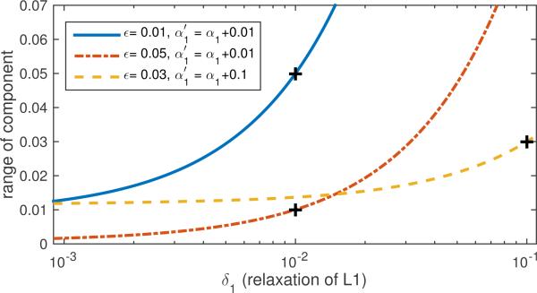
Next we repeated the example but with more relaxed choices for S_DR in the component design, achieved by choosing larger values for α₁. We also used different values for ϵ, the constraint on allowable variation in correlations. The results for three different combinations are given in Fig. 7 for three different combinations of ϵ and α₁. For each example, we chose a new pair of both ${\alpha }_1^{\prime }$ and ϵ, where ${\alpha }_1^{\prime }$ is relaxed by a given amount versus the Basis Pursuit optimal α₁ used in the previous example. We again plotted the performance of these components over increasingly-relaxed versions of S_DR, where we see the features are bounded by the chosen amount of relaxation within the limit given by the chosen ϵ. Further we see that the choice of ϵ and α₁ can control the robustness of the feature beyond the constraint set, as the range of correlations smoothly increase with a curve which depends on the conditions used. This suggests that by carefully designing S_DR, we can calculate components which robustly compute the information we seek.

Figure 7.

p(δ₁) computed via Eq. (12) for component values c^Tx over a relaxed set using three different combinations of δ₁ and ϵ.

3.2. Biomarker Identification from Real fMRI Data

Next we will use the calculated components for finding regions which most accurately classify diseases. We consider a dataset consisting of functional MRI images for a number of subjects which are labeled as cases or controls. We will first use cross-validation to optimize a LASSO regression estimate, in order to find a MAP estimate with the best possible accuracy in differentiating cases versus controls, and this will set the standard we wish to improve on. Then with this as a starting point, we will relax the prior knowledge a controlled amount and use cross-validation to test for improvement in terms of accuracy with unambiguous components. Accuracy is directly computed using the sign of the component score c^Ta_i versus the true class, where a_i is an image in the test set. The goal is to take advantage of the behavior we saw in the simulations as the prior is relaxed, to improve robustness while at the same time maximizing the ability to discriminate cases versus controls.

We used the data from a study comparing psychiatric patients to controls during an auditory sensorimotor task, conducted by The Mind Clinical Imaging Consortium (MCIC) [15]. The study included 208 participants, 92 of whom were diagnosed with schizophrenia, schizophreniform or schizoaffective disorder; the remaining 116 were healthy controls. The fMRI data were preprocessed using the statistical parametric mapping (SPM) software [25]; contrast images associated with the auditory stimuli form the data samples we use. Further details of the data collection and preprocessing can be found in our previous study [7].

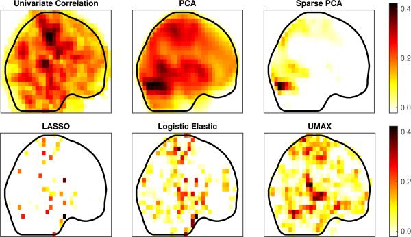
Fig. 8 provides projections of the components or predictors calculated with several different methods. For PCA, Logistic LASSO, and Elastic Net, we used Matlab [16]. The sparse principal component was calculated using the SpaSM toolbox [28], with a setting of 100 nonzero voxels. The regularization parameters for all methods were chosen using 10-fold cross-validation. For UMAX (the proposed method) we started from the norms of the LASSO solution, then performed a line search for the optimal choice of relaxation, and picked the result with highest accuracy.

Figure 8.

Projections of components calculated using: Pearson Correlation, PCA, Sparse PCA, LASSO, Logistic Elastic Net, and UMAX (proposed method).

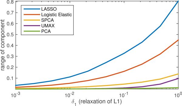
Both the first principal component and the sparse principal component took largest values in the occipital lobe, unlike the supervised methods, suggesting the signal variability was highest there, but not significantly related to the phenotype. The univariate correlation was highest in the precentral and postcentral gyrus, as noted in [7]. This was also evident in the LASSO, Logistic elastic, and UMAX results. The logistic elastic and UMAX result also included more of the neighboring sensory and motor association cortex, and UMAX in particular included a much higher weight to regions of the prefrontal cortex. In Fig. 9 we give the results of testing these components over relaxations of S_DR, suggesting how robust they are to the actual degree of sparsity of the true predictor (measured by relaxations of the ℓ₁-norm). Again we see the controlled ambiguity of the UMAX method. Interestingly, we see that the sparse PCA component had higher ambiguity.

Figure 9.

Component ranges for different elements versus sets of L1-regularized solutions; legend entries are arranged in same order as plot traces, from top to bottom.

To compare the components’ value as biomarkers or for inspiring further research into particular regions, we considered their accuracy at finding regions relevant to the disease. Hence we tested the other features’ classification performance directly by comparing the sign of the feature score c^Ta_i to the sign of b_i, where a_i is a sample in our test set, c is a feature tested, and b_i ∈ {+1, −1} is the phenotype for the sample. In Table 1 we give the best accuracy (defined as the fraction of total test samples which were correctly classified, as used to determine the parameter values) and Pearson correlation achieved by each of the six features in 10-fold cross validation. As expected, we find that the PCA and sparse PCA components are not relevant to the disease. The LASSO solution performed fairly poorly and extensions such as elastic net (which allow a denser solution) and logistic elastic net, yielded minor improvements. Relaxation using the UMAX achieved a more significant improvement, both in terms of accuracy and correlation. We note that the overall accuracies achieved here are in line with meta-analyses [27], which generally suggest accuracies of 65 to 70 percent for samples of this size.

Table 1.

Methods and selectivity of different components compared to disease status.

Method	Accuracy	Correlation
PCA	48.6 %	−0.08
Sparse PCA	54.3 %	0.03
LASSO	62.1 %	0.23
Elastic	62.5 %	0.26
Logistic Elastic	65.4 %	0.31
UMAX	69.2 %	0.35

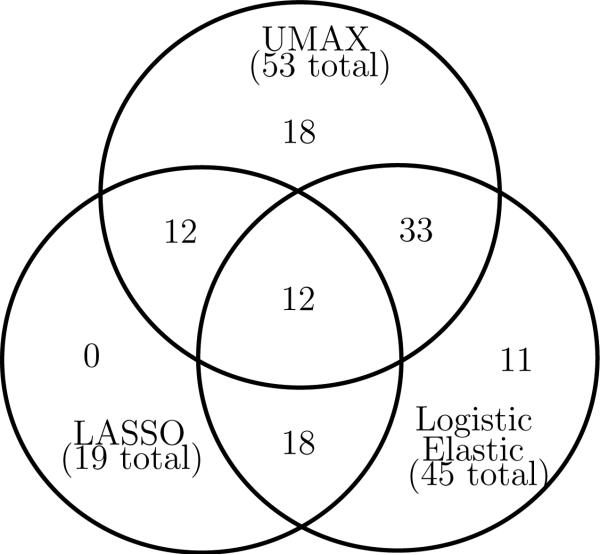
Next we identified the regions of interest (ROI) containing the signal for each of the components, using the Automated Anatomical Labeling (AAL) parcellation [31]. In Fig. 10 we give the number of common and different ROI for the three methods. We see that the elastic net essentially identifies a superset of the LASSO selections, while the proposed method only agrees with about two-thirds of each. Projections of the common and different ROI (for a comparison of UMAX versus logistic elastic net) are provided in Fig. 11, and the names of ROI's are provided in the appendix.

Figure 10.

Intersections and differences in ROI containing the nonzero signal for the different components; the elastic net result is essentially a superset of LASSO, while the UMAX overlaps with roughly two thirds of each.

Figure 11.

Projections of components contained in ROI's common to Logistic Elastic Net and UMAX estimate, and projections of those in only one result but not other.

4. Discussion

In this paper we provided a robust supervised framework for utilizing prior knowledge to find pertinent components of biological mechanisms. We demonstrated promising preliminary results using the technique for neuroimaging data, where we found that the choice of a maximum correlation component provided better accuracy as a classifier of case versus control. The use of the ℓ₁-norm assumes a Laplacian prior, and therefore common significance testing approaches, which presume Gaussian statistics, are not applicable. Hence we used the best accuracy seen in cross-validation as the metric to determine performance. We found a limited degree of relaxation of the prior provides improvement, as the simulations suggested we might, particularly given the fact that the prior appeared to be of limited effectiveness. As the scope of this paper is the introduction of a broadly-applicable method, where many possible forms of prior may be used, we did not delve more deeply into the more specific issues of ℓ₁-regression and associated statistical issues. In future work we intend to focus on both the development of more specialized priors, as well as associated significance testing approaches.

Potential difficulties of the method relate to the computational complexity, both in terms of algorithmic complexity, as well as the number of parameters to be chosen. We can view the latter (indeed all variables except c) as internal variables chosen by the algorithm itself, for example via cross-validation as in the previous section. The advantages of the method result from its rigorous formulation as a combination of dimensionality reduction with prior knowledge. We saw that this provides significant advantage for extremely noisy and underdetermined problems such as classification with neuroimaging data.

HIGHLIGHTS.

• Dimensionality reduction methods like PCA can be viewed as estimates of components constant over all possible unknown mechanisms.

• We derive a method to incorporate a preference for sparsity in the mechanism, while retaining the property of a limited statistical variance over all possible mechanisms.

• The resulting improvement in robustness versus statistical parameters is demonstrated with simulation.

• Components calculated from fMRI demonstrate superior accuracy in classifying schizophrenia.

5. Appendix: ROI Listing

Table 2.

ROI common to UMAX and Logistic Elastic Net.

Postcentral_R	Temporal_Sup_R	Postcentral_L
Frontal_Mid_L	Temporal_Sup_L	Precentral_L
Cingulum_Mid_L	Temporal_Mid_L	Paracentral_Lobule_L
Cuneus_L	Precuneus_L	Precuneus_R
Cerebelum_6_L	Frontal_Sup_R	Parietal_Sup_R
Calcarine_L	Cingulum_Post_L	Cerebelum_6_R
Frontal_Sup_Medial_L	Supp_Motor_Area_R	Cerebelum_Crusl_L
Frontal_Inf_Tri_R	Frontal_Med_Orb_R	Temporal_Pole_Sup_L
Cerebelum_4_5_R	Fusiform_R	Lingual_L
Occipital_Mid_L	Paracentral_Lobule_R	Temporal_Mid_R
Lingual_R	Rolandic_Oper_L	Caudate_R

Table 3.

ROI in either UMAX or Logistic Elastic Net which is not common to other.

UMAX Only	Logistic Elastic Only
Frontal_Mid_R	Parietal_Inf_L
Precentral_R	Olfactory_L
Temporal_Inf_R	Insula_R
Frontal_Med_Orb_L	Caudate_L
Cerebelum_Crus2_L	Parietal_Sup_L
ParaHippocampal_R	Putamen_L
Supp_Motor_Area_L	Thalamus_R
Cingulum_Ant_L	Cerebelum_3_R
Olfactory_R	SupraMarginal_R
Parietal_Inf_R	Rolandic_Oper_R
Frontal_Sup_Orb_L	Temporal_Pole_Sup_R
Fusiform_L	Hippocampus_L
Frontal_Sup_Orb_R
Cerebelum_4_5_L
SupraMarginal_L
Calcarine_R
Frontal_Inf_Orb_L
Cingulum_Mid_R
Rectus_R
Insula_L

References

- 1.De Angelis Pasquale L., Pardalos Panos M., Toraldo Gerardo. Quadratic Programming with Box Constraints. In: Bomze Immanuel M., Csendes Tibor, Horst Reiner, Pardalos Panos M., editors. Developments in Global Optimization, number 18 in Nonconvex Optimization and Its Applications. Springer; US: 1997. pp. 73–93. [Google Scholar]
- 2.Bair Eric, Hastie Trevor, Paul Debashis, Tibshirani Robert. Prediction by Supervised Principal Components. Journal of the American Statistical Association. 2006 Mar;101(473):119–137. [Google Scholar]
- 3.Barshan Elnaz, Ghodsi Ali, Azimifar Zohreh, Zolghadri Jahromi Mansoor. Supervised principal component analysis: Visualization, classification and regression on subspaces and submanifolds. Pattern Recognition. 2011 Jul;44(7):1357–1371. [Google Scholar]
- 4.Boyd Stephen P., Vandenberghe Lieven. Convex Optimization. Cambridge University Press; Mar, 2004. [Google Scholar]
- 5.Buck Stuart, reproducibility Solving. Science. 2015 Jun;348(6242):1403–1403. doi: 10.1126/science.aac8041. [DOI] [PubMed] [Google Scholar]
- 6.Cao Hongbao, Duan Junbo, Lin Dongdong, Yao Shugart Yin, Calhoun Vince, Wang Yu-Ping. Sparse representation based biomarker selection for schizophrenia with integrated analysis of fMRI and SNPs. NeuroImage. 2014 Nov;102(Pt 1):220–228. doi: 10.1016/j.neuroimage.2014.01.021. [DOI] [PMC free article] [PubMed] [Google Scholar]
- 7.Chen Jiayu, Calhoun Vince D., Pearlson Godfrey D., Ehrlich Stefan, Turner Jessica A., Ho Beng-Choon, Wassink Thomas H., Michael Andrew M., Liu Jingyu. Multifaceted genomic risk for brain function in schizophrenia. NeuroImage. 2012 Jul;61(4):866–875. doi: 10.1016/j.neuroimage.2012.03.022. [DOI] [PMC free article] [PubMed] [Google Scholar]
- 8.Shaobing Chen Scott, Donoho David L., Saunders Michael A. Atomic Decomposition by Basis Pursuit. SIAM Review. 2001 Jan;43(1):129–159. [Google Scholar]
- 9.Chu Carlton, Hsu Ai-Ling, Chou Kun-Hsien, Bandettini Peter, Lin ChingPo. Does feature selection improve classification accuracy? Impact of sample size and feature selection on classification using anatomical magnetic resonance images. NeuroImage. 2012 Mar;60(1):59–70. doi: 10.1016/j.neuroimage.2011.11.066. [DOI] [PubMed] [Google Scholar]
- 10.Dillon Keith, Fainman Yeshaiahu. Bounding pixels in computational imaging. Applied Optics. 2013 Apr;52(10):D55–D63. doi: 10.1364/AO.52.000D55. [DOI] [PubMed] [Google Scholar]
- 11.Dillon Keith, Fainman Yeshaiahu. Element-wise uniqueness, prior knowledge, and data-dependent resolution. Signal, Image and Video Processing. 2016 Apr;:1–8. [Google Scholar]
- 12.Dillon Keith, Wang Yu-Ping. Imposing uniqueness to achieve sparsity. Signal Processing. 2016 Jun;123:1–8. doi: 10.1016/j.sigpro.2015.12.009. [DOI] [PMC free article] [PubMed] [Google Scholar]
- 13.Dunteman George H. Principal Components Analysis. SAGE; May, 1989. [Google Scholar]
- 14.Gill Philip E., Murray Walter, Wright Margaret H. Numerical linear algebra and optimization. Addison-Wesley Pub. Co., Advanced Book Program; 1991. [Google Scholar]
- 15.Gollub Randy L., Shoemaker Jody M., King Margaret D., White Tonya, Ehrlich Stefan, Sponheim Scott R., Clark Vincent P., Turner Jessica A., Mueller Bryon A., Magnotta Vince, OLeary Daniel, Ho Beng C., Brauns Stefan, Manoach Dara S., Seidman Larry, Bustillo Juan R., Lauriello John, Bockholt Jeremy, Lim Kelvin O., Rosen Bruce R., Charles Schulz S, Calhoun Vince D., Andreasen Nancy C. The MCIC collection: a shared repository of multi-modal, multi-site brain image data from a clinical investigation of schizophrenia. Neuroinformatics. 2013 Jul;11(3):367–388. doi: 10.1007/s12021-013-9184-3. [DOI] [PMC free article] [PubMed] [Google Scholar]
- 16.Grace Andrew. MATLAB optimization Toolbox. The MathWorks Inc.; Natick, USA: 1992. [Google Scholar]
- 17.Guyon Isabelle, Elisseeff Andr. An Introduction to Variable and Feature Selection. J. Mach. Learn. Res. 2003 Mar;3:1157–1182. [Google Scholar]
- 18.Kowalski Matthieu. Sparse regression using mixed norms. Applied and Computational Harmonic Analysis. 2009 Nov;27(3):303–324. [Google Scholar]
- 19.Krystal John H., State Matthew W. Psychiatric Disorders: Diagnosis to Therapy. Cell. 2014 Mar;157(1):201–214. doi: 10.1016/j.cell.2014.02.042. [DOI] [PMC free article] [PubMed] [Google Scholar]
- 20.Lemm Steven, Blankertz Benjamin, Dickhaus Thorsten, Mller Klaus-Robert. Introduction to machine learning for brain imaging. NeuroImage. 2011 May;56(2):387–399. doi: 10.1016/j.neuroimage.2010.11.004. [DOI] [PubMed] [Google Scholar]
- 21.Lin Dongdong, Cao Hongbao, Calhoun Vince D., Wang Yu-Ping. Sparse models for correlative and integrative analysis of imaging and genetic data. Journal of Neuroscience Methods. 2014 Nov;237:69–78. doi: 10.1016/j.jneumeth.2014.09.001. [DOI] [PMC free article] [PubMed] [Google Scholar]
- 22.Ma Shuangge, Dai Ying. Principal component analysis based methods in bioinformatics studies. Briefings in Bioinformatics. 2011 Nov;12(6):714–722. doi: 10.1093/bib/bbq090. [DOI] [PMC free article] [PubMed] [Google Scholar]
- 23.Milliken George A., Johnson Dallas E. Analysis of Messy Data Volume 1: Designed Experiments. Second Edition CRC Press; Mar, 2009. [Google Scholar]
- 24.Orr Graziella, Pettersson-Yeo William, Marquand Andre F., Sartori Giuseppe, Mechelli Andrea. Using Support Vector Machine to identify imaging biomarkers of neurological and psychiatric disease: A critical review. Neuroscience & Biobehavioral Reviews. 2012 Apr;36(4):1140–1152. doi: 10.1016/j.neubiorev.2012.01.004. [DOI] [PubMed] [Google Scholar]
- 25.Penny William D., Friston Karl J., Ashburner John T., Kiebel Stefan J., Nichols Thomas E. Statistical Parametric Mapping: The Analysis of Functional Brain Images: The Analysis of Functional Brain Images. Academic Press; Apr, 2011. [Google Scholar]
- 26.Radhakrishna Rao C, Toutenburg Helge. Linear Models: Least Squares and Alternatives. Springer Science & Business Media; Jun, 2013. [Google Scholar]
- 27.Schnack Hugo G., Kahn Ren S. Detecting Neuroimaging Biomarkers for Psychiatric Disorders: Sample Size Matters. Neuroimaging and Stimulation. 2016:50. doi: 10.3389/fpsyt.2016.00050. [DOI] [PMC free article] [PubMed] [Google Scholar]
- 28.Sjstrand Karl, Harder Clemmensen Line, Larsen Rasmus, Ersbll Bjarne. Spasm: A matlab toolbox for sparse statistical modeling. Journal of Statistical Software Accepted for publication. 2012 [Google Scholar]
- 29.Tibshirani Robert. Regression shrinkage and selection via the lasso. Journal of the Royal Statistical Society. Series B (Methodological) 1996:267–288. [Google Scholar]
- 30.Tibshirani Ryan J. The lasso problem and uniqueness. Electronic Journal of Statistics. 2013;7:1456–1490. [Google Scholar]
- 31.Tzourio-Mazoyer N, Landeau B, Papathanassiou D, Crivello F, Etard O, Delcroix N, Mazoyer B, Joliot M. Automated anatomical labeling of activations in SPM using a macroscopic anatomical parcellation of the MNI MRI single-subject brain. NeuroImage. 2002 Jan;15(1):273–289. doi: 10.1006/nimg.2001.0978. [DOI] [PubMed] [Google Scholar]
- 32.Yuan Ming, Lin Yi. Model selection and estimation in regression with grouped variables. Journal of the Royal Statistical Society: Series B (Statistical Methodology) 2006 Feb;68(1):49–67. [Google Scholar]
- 33.Zhang Hui, Yin Wotao, Cheng Lizhi. Necessary and Sufficient Conditions of Solution Uniqueness in 1-Norm Minimization. Journal of Optimization Theory and Applications. 2014 Aug;164(1):109–122. [Google Scholar]
- 34.Zou Hui, Hastie Trevor. Regularization and variable selection via the Elastic Net. Journal of the Royal Statistical Society, Series B. 2005;67:301–320. [Google Scholar]
- 35.Zou Hui, Hastie Trevor, Tibshirani Robert. Sparse Principal Component Analysis. Journal of Computational and Graphical Statistics. 2006 Jun;15(2):265–286. [Google Scholar]