Abstract
Limitations of many Brain Machine Interface (BMI) systems using invasive electrodes include reliance on single neurons and decoding limited to kinematics only. This study investigates whether force-related information is present in the local field potential (LFP) recorded with deep brain electrodes using data from 14 patients with Parkinson’s disease. A classifier based on logistic regression (LR) is developed to classify various force stages, using 10-fold cross validation. Least Absolute and Shrinkage Operator (Lasso) is then employed in order to identify the features with the most predictivity. The results show that force-related information is present in the LFP, and it is possible to distinguish between various force stages using certain frequency-domain (delta, beta, gamma) and time-domain (mobility) features in real-time.
I. Introduction
An important objective of Brain-Machine Interface (BMI) research is to improve neural control of limb prostheses to help people with movement disorders (e.g. Parkinson’s disease), or those affected by amputation or paralysis (e.g. due to stroke, amyotrophic lateral sclerosis). The majority of previous BMI systems have relied on neural spiking for decoding movement related information from cortical areas of the brain. The problem with spike recordings is the lack of longevity due to either dying of neurons or change in the micro-movement [1]. Local Field Potentials (LFP) recorded have demonstrable longevity [2]. Few studies have used LFP for decoding movement related information in monkeys and human subjects [3]. However, most decode kinematics (position and velocity of limbs) without attempting to decode the forces causing the movement or used in gripping [4]. The aim of this study is to investigate whether force-related information is present in the LFP, and whether it is possible to distinguish between various stages of manual gripping (i.e. force onset, force development, and force release) using a classification algorithm. Furthermore, the study also aims to identify the key features in the LFP that provide the most force-related information in the LFP. In this study, we have used data from 14 subjects with Parkinson’s disease.
II. Methods
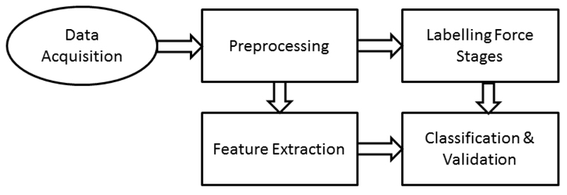
Figure 1 shows an overview of the various steps undertaken in the study. In this section, we will describe how the data were acquired (Experimental Paradigm & Recordings), how various force stages were identified (Labelling of Force Stages), the various features that were extracted both in time-domain and frequency domain (Feature Extraction) and finally the classification algorithm employed while using a feature reduction technique with cross validation to identify the key features (Classification & Validation).
Figure 1.
Overview of the methods employed
A. Experimental Paradigm & Recordings
Patients were presented with a series of visual cues (a light emitting diode turning on for 5 seconds) and instructed to squeeze a force dynamometer as hard and as fast as possible for the duration of the light being on. About half of the visual cues were accompanied with loud auditory stimuli, delivered via headphones, although patients were still advised to focus on the visual cue alone. On average, a total of 20 trials were collected in each experimental run, using either hand. For each patient, the experiment was undertaken with both hands, in turns. Recordings were undertaken 3-6 days after surgery, first after overnight withdrawal of antiparkinsonian medication, and then ~1 hour after the usual dose of medication. The LFPs were recorded using either a D360 amplifier (Digitimer Ltd) in combination with a 1401 A/D converter (Cambridge Electronic Design), or a TMSi porti (TMS international). Using adjacent contacts of each deep brain stimulation electrode targeting the subthalamic nucleus (STN, part of basal ganglia in the brain), bipolar LFPs (0-1, 1-2, 2-3) were recorded, providing 3 bipolar channels each for the right and left STN. This paradigm is explained in greater detail in [5].
A total of 14 patients with Parkinson’s disease gave informed consent and took part in the study, amounting to 1,101 trials. The study was approved by the local ethics committees at recording sites in Oxford and London, UK. All the signals were acquired using Spike 2 software (Cambridge Electronic Design), which were later imported into Matlab 2013b (Mathworks Inc) for subsequent analysis. For each patient, a separate experiment was conducted for each hand, with and without medication so that there were a total of 56 recording sessions. The breakdown of trials according to medication (whether prior to medication (No Medication) or after a dose of L-Dopa (ON Medication)), stimuli type (visual only (V) or visual accompanied by auditory signal (AV)), and whether left hand or right hand is given in Table 1.
Table 1. Number of Trials in Total Across all the 14 Patients, in Various Situations.
| V, Left | AV, Left | V, Right | AV, Right | |
|---|---|---|---|---|
| No Medication | 127 | 138 | 123 | 152 |
| ON Medication | 127 | 159 | 121 | 154 |
B. Preprocessing
All the patients’ data were first imported into Matlab, and resampled to 512 Hz to ensure uniformity across the dataset. For each trial, a 9-second epoch was extracted with 2 seconds before the light turned on, and 7 seconds after this. The LFP from the 3 bipolar channels on each side (0-1, 1-2, 2-3) was subsequently convolved with a complex Morlet wavelet [6]. Convolution with an appropriate wavelet enabled the transformation of the time-domain LFP signal into a time-frequency signal, allowing us to determine power in various frequency bands over time. In the wavelet transform, we used a linear frequency scale ranging from 3 Hz to 200 Hz (198 frequency points) and a variable number of cycles (4 to 10, as a function of frequency).
C. Labelling of Force Stages
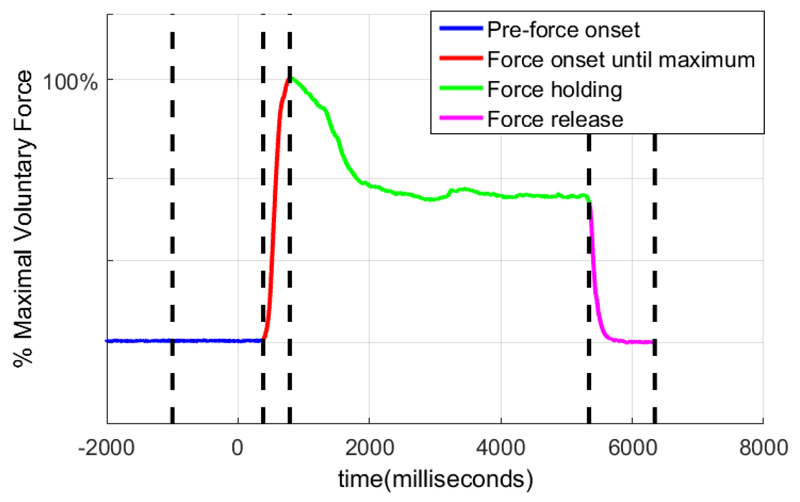
Figure 2 shows a typical force profile, as measured by the force dynamometer with the various stages automatically determined using a heuristic algorithm. The force onset was determined by searching forward, starting from stimuli onset until a threshold, thresholdonset, was exceeded for at least 15 samples. The thresholdonset was determined using equations (1-3) where f(x) refers to the force value at time = x, and mean(y), std(y) refer to the mean and standard deviation of y respectively. The time values were expressed in milliseconds (ms), and f(−1200: −200) refers to the force value from 1200 ms to 200 ms before the stimuli.
| (1) |
| (2) |
| (3) |
Figure 2.
A typical force profile, with various stages automatically determined with a heuristic algorithm
Next, the maximum value of force was determined, by searching for the maximum force value during the trial (time = 0 ms to time = 5000 ms). Subsequently, the time when the patient released force was determined by searching forward from time = 3000ms until the force value remained below a threshold, thresholdrelease for at least 15 samples. The thresholdrelease was determined using equations (4-6).
| (4) |
| (5) |
| (6) |
This identified the various force segments: Forcepre–onset (a second before stimulus onset until the onset of force shown in blue), Forceonset–max (from onset of force until the force maximum, shown in red), Forceholding (from maximum force until the point of force release shown in green), and Forcerelease (from the point of force release until a fixed point at the end of the trial, shown in magenta) as illustrated in Figure 2.
D. Feature Extraction
A 256 millisecond long sliding window, with an overlap of 16 milliseconds was used in order to extract various frequency-domain and time-domain features. In order to exploit information from all channels, the features were extracted from the 3 bipolar channels on each side and then averaged, for a given sliding window.
Frequency-domain features
Power in ten different frequency bands ranging from 3 Hz to 200 Hz was identified as potential frequency domain features. Similar to the approach adopted in [7], we identified 10 distinct frequency bands: delta (3-4 Hz), theta (4-8 Hz), alpha (8-14 Hz), beta1 (14-20 Hz), beta2 (20-30 Hz), gamma1 (30-50 Hz), gamma2 (50-90 Hz), gamma3 (90-120 Hz), gamma4 (120-150 Hz), and gamma5 (150-200 Hz). Before extraction of power in these bands, a baseline normalization was performed on each trial using equations (7-8) where tfnormk is the normalized time-frequency function of the kth trial, trialmean is the mean of N trials for a single patient, and tfk (−2000: −550, f) is the time-frequency function of the kth trial from 2000 ms to 500 ms before stimulus onset, at a frequencyf.
| (7) |
| (8) |
The baseline normalization allowed us to express any force-related changes in the LFP as a percentage change with respect to the pre-stimulus LFP, thereby removing the effects of any background activity and allowing comparison across sides and patients.
Time-domain features
Hjorth [8] proposed three metrics characterizing the amplitude/time pattern of electroencephalograms. These were anticipated to capture statistical properties of the LFP signal in each time-window, which might otherwise not be captured by frequency band power. The three proposed metrics were activity (a measure of the variance of the signal, equivalent to the total power in the frequency domain), mobility (a measure of the standard deviation of the slope of the original signal relative to the standard deviation of the signal which is equivalent to the standard deviation of the power spectrum along the frequency axis), and complexity (a measure of the smoothness of the signal with reference to the ‘softest’ signal, i.e. sine wave, computed using the standard deviation of the second derivative) [8].
E. Classification & Validation
In this work, we used a logistic regression based classification to differentiate between two classes, a special case of generalized linear model which is easily interpretable and one of the most widely used classification algorithms in machine learning [9]. In the two class classification problem, one class is typically labelled as 0, while the other class is labelled as 1. The hypothesis function used in logistic regression is given in equation (7) where xn and Ɵn are the nth normalized feature and parameter respectively, and g(y) is a sigmoid function (equation 8) thereby forcing the weighted linear combination of different features to range from 0 to 1 lending itself to be interpreted as probability.
| (7) |
| (8) |
Each of the xn features was normalized to zero mean and unit variance. The main component of a classification algorithm is determining the parameters in the hypothesis function that minimize a cost function. The cost function for logistic regression is shown in equation (9), where m is the total number of training points. The cost function outputs a large value when the predicted value, hƟ(x) is very different from the true class value,y, and a very small output when the predicted value is close to the true class value.
| (9) |
One technique to reduce the large feature space and make the model more interpretable is appropriate regularization. In regularization, an additional term is added to the cost function which is dependent only on the estimated parameters to guard against overfitting by penalizing for large parameter values. In this study, we used the l1 norm parametrized by λ as the regularization parameter. The advantage of using the l1 norm as opposed to other forms of regularization terms (e.g. l2 norm used in ridge regression) is that it results in sparse solution i.e. forces the less important features to 0. The amount of regularization is controlled by λ and by iterating through different values of lambda, we can generate a large number of models with varying degree of regularization. With increasing λ, increasing number of features will be forced to 0 and vice versa. This technique is called LASSO (least absolute shrinkage and selection operator) [10], and helps to determine the important features for a classification task.
To ensure generalization, we used a 10-fold cross validation, using a single fold for testing each time while using the remaining 9 folds for training. We selected the optimal model during LASSO by plotting the cross validation error on the testing set along with error bars, and finding the model with the highest λ which was within 1 standard error of the point of minimum cross validation error, the “1SE” rule [11]. This is effectively equivalent to choosing the most regularized model (the simplest model) which is within 1 standard error of the minimum error.
III. Results
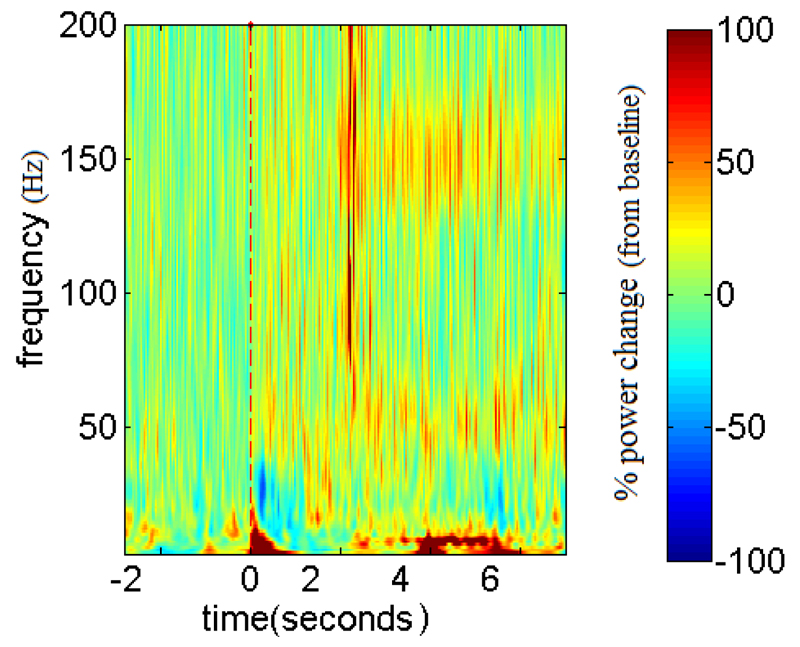
Figure 3 shows the mean time-frequency plot (normalized with baseline) from a single recording session of a patient. There is increased power in the low frequency band, a reduction of power in the beta band, and increased power in the gamma band beginning soon after the stimulus onset (t = 0 ms).
Figure 3.
Mean time-frequency plot of a single patient on medication, averaged across all the trials with AV stimuli
We aimed to investigate whether we could correctly distinguish various force stages using LFP recorded from electrodes targeting the STN. These were detection of force onset (Forcepre–onset vs Forceonset–max) labelled as “Pre vs Dev”, force development versus force constant (Forceonset–max vs Forceholding) labelled as “Dev vs Stab” and force development versus force release (Forceonset–max vs Forcerelease) labelled as “Dev vs Rel”. We also aimed to identify the key features employed in these classification tasks.
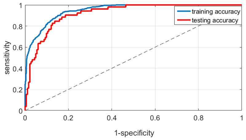
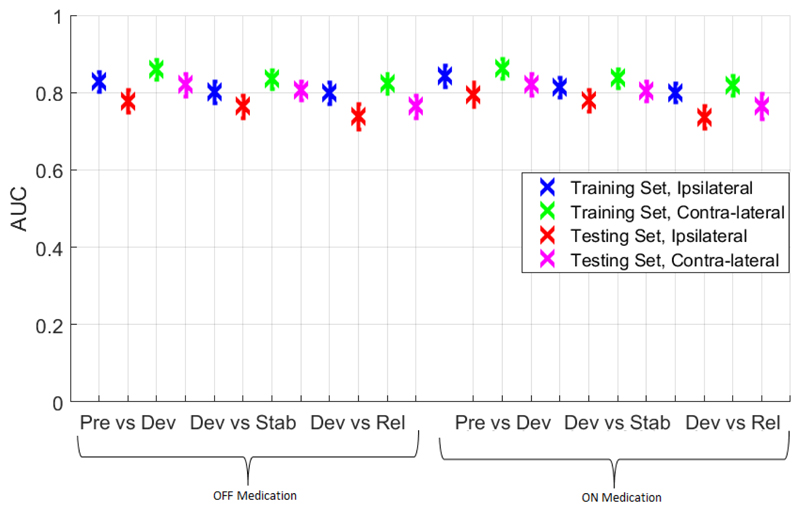
Figure 4 shows the training and testing accuracy using a Receiver Operating Characteristic (ROC) curve for a single patient, while attempting to distinguish Forcepre–onset from Forceonset–max, using a 10-fold cross validation and a logistic regression based classifier (without regularization). We used a similar approach to compute the AUC (Area Under the Curve) for each of the classification tasks, across all 14 patients. For each patient, there were 2 contralateral sessions without medication and 2 with medication, and similarly 4 ipsilateral sessions. This afforded a total of 112 sessions with 28 in each situation (ipsilateral or contralateral with or without medication). Table 2 shows the mean and the 25th and 75th percentile AUC in each situation across the population and Figure 5 shows the same for both training and testing, along with error bars. These results show that the classification performance using LFP from the contralateral STN was consistently better than that using LFP from the ipsilateral STN. In addition, the performance of the classification tasks did not depend on medication. It was slightly easier to distinguish between Forcepre–onset and Forceonset–max, and between Forceonset–max and Forceholding as opposed to distinguishing between Forceonset–max and Forcerelease.
Figure 4.
ROC curve to distinguish between Forcepre–onset and Forceonset–max , for a single patient using a 10-fold cross validation and a logistic regression based classification technique (Training AUC: 0.949, Testing AUC: 0.921)
Table 2. Mean (25th – 75th percentile) AUC across all patients using a logistic regression based classifier with 10-fold cross validation under various situations.
| Without medication | On medication | |||
|---|---|---|---|---|
| Ipsilateral | Contralateral | Ipsilateral | Contralateral | |
| Pre vs Dev | 0.778 (0.69-0.85) | 0.821 (0.76-0.90) | 0.796 (0.73-0.86) | 0.821 (0.76-0.91) |
| Dev vs Stab | 0.764 (0.68-0.88) | 0.806 (0.74-0.86) | 0.779 (0.71-0.84) | 0.804 (0.72-0.87) |
| Dev vs Rel | 0.738 (0.67-0.81) | 0.765 (0.72-0.86) | 0.737 (0.66-0.79) | 0.765 (0.70-0.85) |
Figure 5.
Mean AUC in various situations across all patients for “Pre vs Dev”, “Dev vs Stab”, and “Dev vs Rel” using a logistic regression based classifier with 10-fold cross validation
Lastly, using the LASSO approach, we identified the key features for each of the classification tasks using data from all the patients, as shown in Table 3. The features are listed in a descending order, based on the magnitude of Ɵ corresponding to each feature.
Table 3. Important features identified in each of the classification task, using LASSO.
| Important Features identified with LASSO | |
|---|---|
| Pre vs Dev | Mobility, Gamma2, Beta1, Beta2, Gamma1 |
| Dev vs Stab | Mobility, Delta, Beta1, Alpha, Gamma2 |
| Dev vs Rel | Mobility, Delta, Gamma2, Gamma1, Beta2 |
IV. Discussion & Conclusion
We showed that there is indeed force information present in the LFP, and it is possible to distinguish between various force stages using a machine learning approach. This study also found that in addition to the frequency bands (delta, beta and gamma), mobility is also an important feature that can usefully be incorporated in any BMI system aiming to control force using the STN LFP. We are not aware of any previous work that has classified various force stages using LFP but the classification results with AUC as high as 0.8 across patients with Parkinson’s disease are promising. Furthermore, the classification task was based on using a short sliding window, suggesting that it is possible to decode force-related information from LFP with minimal latency, in real time. Future work will investigate whether it is possible to predict the absolute value of force from the LFP (regression) during various tasks rather than to predict only a finite number of stages (classification).
Acknowledgment
The authors would like to acknowledge Anam Anzak who collected the data and all the patients who took part in the study.
References
- 1.Hall TM, Nazarpour K, Jackson A. Real-time estimation and biofeedback of single-neuron firing rates using local field potentials. Nature communications. 2014;5 doi: 10.1038/ncomms6462. [DOI] [PMC free article] [PubMed] [Google Scholar]
- 2.Giannicola G, et al. Subthalamic local field potentials after seven-year deep brain stimulation in Parkinson's disease. Experimental neurology. 2012;237(2):312–317. doi: 10.1016/j.expneurol.2012.06.012. [DOI] [PubMed] [Google Scholar]
- 3.Mamun K, et al. Movement decoding using neural synchronization and inter-hemispheric connectivity from deep brain local field potentials. Journal of neural engineering. 2015;12(5):056011. doi: 10.1088/1741-2560/12/5/056011. [DOI] [PubMed] [Google Scholar]
- 4.Bensmaia SJ, Miller LE. Restoring sensorimotor function through intracortical interfaces: progress and looming challenges. Nature reviews Neuroscience. 2014;15(5):313–325. doi: 10.1038/nrn3724. [DOI] [PubMed] [Google Scholar]
- 5.Anzak A, et al. Subthalamic nucleus activity optimizes maximal effort motor responses in Parkinson’s disease. Brain. 2012 doi: 10.1093/brain/aws183. p. aws183. [DOI] [PMC free article] [PubMed] [Google Scholar]
- 6.Cohen MX. Analyzing neural time series data: theory and practice. MIT Press; 2014. [Google Scholar]
- 7.Chen C, et al. Decoding grasp force profile from electrocorticography signals in non-human primate sensorimotor cortex. Neuroscience research. 2014;83:1–7. doi: 10.1016/j.neures.2014.03.010. [DOI] [PubMed] [Google Scholar]
- 8.Hjorth B. EEG analysis based on time domain properties. Electroencephalography and clinical neurophysiology. 1970;29(3):306–310. doi: 10.1016/0013-4694(70)90143-4. [DOI] [PubMed] [Google Scholar]
- 9.Dreiseitl S, Ohno-Machado L. Logistic regression and artificial neural network classification models: a methodology review. Journal of biomedical informatics. 2002;35(5):352–359. doi: 10.1016/s1532-0464(03)00034-0. [DOI] [PubMed] [Google Scholar]
- 10.Tibshirani R. Regression shrinkage and selection via the lasso. Journal of the Royal Statistical Society. Series B (Methodological) 1996:267–288. [Google Scholar]
- 11.Hastie T, et al. The elements of statistical learning: data mining, inference and prediction. The Mathematical Intelligencer. 2005;27(2):83–85. [Google Scholar]


