Visualization of cortical, subcortical, and deep brain neural circuit dynamics during naturalistic mammalian behavior with head-mounted microscopes and chronically implanted lenses

Abstract

Genetically encoded calcium indicators for visualizing dynamic cellular activity have greatly expanded our understanding of the brain. However, due to light scattering properties of the brain as well as the size and rigidity of traditional imaging technology, in vivo calcium imaging has been limited to superficial brain structures during head fixed behavioral tasks. This limitation can now be circumvented by utilizing miniature, integrated microscopes in conjunction with an implantable microendoscopic lens to guide light into and out of the brain, thus permitting optical access to deep brain (or superficial) neural ensembles during naturalistic behaviors. Here, we describe procedural steps to conduct such imaging studies using mice. However, we anticipate the protocol can be easily adapted for use in other small vertebrates. Successful completion of this protocol will permit cellular imaging of neuronal activity and the generation of data sets with sufficient statistical power to correlate neural activity with stimulus presentation, physiological state, and other aspects of complex behavioral tasks. This protocol takes 6–11 weeks to complete.

Introduction

Methodologies for monitoring neural activity in vivo, such as electrophysiology^1,2, neurochemical measurements^3,4, and optical imaging of fluorescently reported neural dynamics^5–8 have substantially increased our understanding of the neural computations underlying complex behavioral states. Among these techniques, the development and implementation of genetically-encoded Ca²⁺ indicators (GECI)^6,9–13 have been particularly advantageous to the study of brain function. During periods of heightened neural activity^14,15, Ca²⁺ flows into the dendritic branches¹⁶ and cell bodies of neurons, increasing intracellular concentrations of Ca²⁺. These activity dependent fluctuations in intracellular Ca²⁺ can be monitored by introducing a Ca²⁺ indicator, such as GCaMP¹³, into the neuronal population of interest. Upon the binding of Ca²⁺, indicators of Ca²⁺ emit a fluorescent signal, which is intensified during periods of elevated neural activity^14,15. As a result, fluctuations in fluorescent emission over time can be used to infer dynamic changes in cellular activity. Moreover, when these signals are visualized with cellular-level resolution, fluorescent indicators of neural activity provide not only temporal information related to dynamic changes in brain cell activity¹⁷, but they also enable the visualization of each cells spatial location within the brain¹⁸.

The visualization of fluorescently reported neural signals within the brain requires both a light source to excite the Ca²⁺ indicator as well as a light-sensing device to detect the emission signal¹⁹. As a result, optical monitoring of fluorescently reported neural activity is constrained by physical limitations to transmit light to and from the neuron population of interest. Specifically, neural tissue exhibits high levels of light scattering and this physical property has precluded optical imaging of in vivo Ca²⁺ transients within deep brain regions¹⁹. However, limitations in the propensity to transmit light through the brain can be circumvented by the implantation of a microendoscopic lens (gradient refractive index (GRIN) lenses attached on either end of a relay lens) in subcortical or deep brain regions^20–22 (Fig. 1a). Microendoscopic lenses facilitate the visualization of deep brain neural activity by relaying light to and from deep brain structures, bringing previously inaccessible fluorescence signals into a field of view outside the brain^11,23–25. For example, these lenses have been utilized to visualize the activity of genetically defined neurons located within deep brain regions, such as the hypothalamus, thus greatly expanding the population of neurons that can be visualized and monitored within the brain^26,27.

Figure 1. Freely behaving Ca²⁺ imaging.

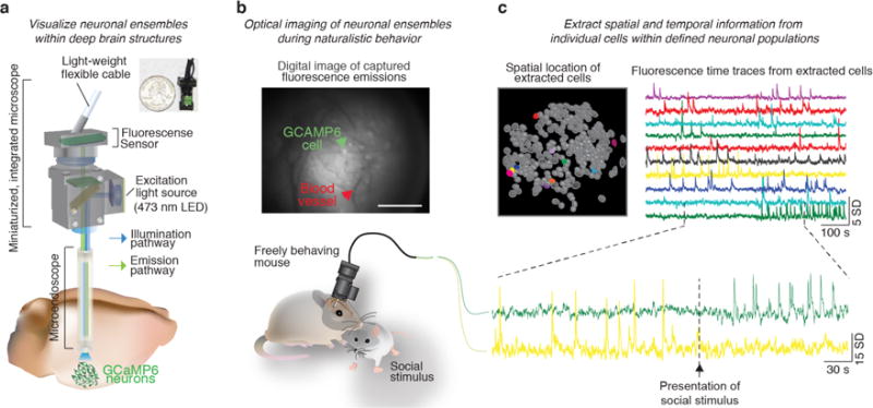
(a) Cartoon diagram of a miniature, integrated microscope containing all optical components necessary for the visualization of fluorescently encoded Ca²⁺ transients in freely behaving mice. Specifically, the microscope contains an excitation light source (473 nm LED), lenses for guiding and focusing light, a fluorescence sensor to detect emission light, and is small enough to fit on the head of a mouse (inset shows actual size of microscope). To visualize neural activity within deep brain regions, this microscope can be used in conjunction with a microendoscope chronically implanted in the brain to bring the activity of GCaMP expressing neurons above the surface of the brain. (b) Example of digitally captured fluorescence activity from the brain of a freely behaving mouse. The green arrow points to a GCaMP6 expressing neuron and the red arrow points to a clearly visualized blood vessel. Scale bar = 123 μm. (c) Example data extracted from digitally captured fluorescence signals. Image on left shows the spatial location of identified cells and traces to the right show changes in fluorescence signal over time, represented as the variance from the mean fluorescence signal at each time point. Zoomed in portion of traces shows example Ca²⁺ activity traces from a cell that increased firing (top, green) and an example of a cell that decreased firing (bottom, yellow) in response to the presentation of a social stimulus. Representative data were collected from one mouse in one acute recording session. All procedures were approved by Intuitional Animal Care and Use Committee (IACUC) at UNC.

Due to the size and rigidity of traditional imaging technology, previous imaging studies have also been limited in the types of behaviors that could be examined, and therefore the scientific questions that could be asked. However, the miniaturization of optical imaging technology, such as the development of miniature, integrated microscopes, which are small and light enough to be carried on the head of the animal without interfering with behavior has greatly expanded the scope of scientific questions that can be asked²⁸. Importantly, these miniature microscopes can be utilized in conjunction with microendoscopic lenses, permitting access to deep brain neural computations associated with naturalistic animal behavior (Fig 1a)^22,26,27. An additional advantage of this technique is that it can be used to repeatedly visualize large-scale neuronal populations (up to a thousand neurons in one mouse²⁹), providing a significant increase in statistical power over previously developed in vivo recording methods. Here, we provide a detailed protocol for the surgical implantation of a microendoscopic lens above a deep brain (or superficial) neuron population and the subsequent collection of in vivo imaging data in a freely behaving mouse (Fig 1b,c). These procedures have been developed and used by our laboratory to maximize imaging success rate during active, naturalistic, animal behaviors²⁶.

Comparison with other in vivo recording methods

One commonly used approach to image fluorescently reported neuronal dynamics is 2-photon microscopy³⁰. This technique utilizes low energy near infrared (IR) photons to penetrate highly light-scattering brain tissue up to 600–700 μm below the surface of the brain³¹. A significant advantage of 2-photon microscopy is the ability to selectively excite fluorophores within a well-defined focal plane, resulting in a spatial resolution capable of resolving cellular activity within precisely defined anatomical sub-regions of neurons, such as dendrites and axonal boutons³⁰. Notably, although this imaging modality provides superior spatial resolution, it requires the head fixation of animals and, in the absence of a microendoscope or optical cannula, 2-photon imaging is limited to superficial layers of the brain^32,33. Together, these behavioral and optical limitations greatly reduce the scope of scientific questions that can be examined with 2-photon microscopy.

Implantation of small, lightweight fiber optics above a region of interest, such as with fiber photometry, circumvents optical and behavioral limitations posed by 2-photon microscopy³⁴. However, unlike 2-photon microscopy, fiber photometry lacks cellular level resolution and provides only aggregate activity within the field of view (i.e., bulk changes in fluorescent signal)²². Thus, this method is better suited for monitoring dynamic activity within neural projection fields³⁵. In addition to limitations in optical resolution, fiber photometry requires the test subject to be secured to a rigid fiber optic bundle, which can be difficult for small mammals, such as mice, to maneuver³⁴. Thus, while fiber photometry increases the depth in which neural activity can be monitored, it presents significant limitations in optical resolution, restricts the natural behavioral repertoire of an animal, and limits the animal models that can be optimally utilized.

Large-scale recordings of neural activity within freely behaving mammals³⁶ can also be conducted with techniques that do not rely on the use of fluorescence indicators of neural activity, such as in vivo electrophysiological recordings². Importantly, compared to in vivo Ca²⁺ imaging, electrophysiology provides superior temporal resolution, allowing for more accurate spike timing estimations^17,37,38 as well as the correlation of neural activity with precisely defined temporal events. In addition, in vivo electrophysiology can be combined with optogenetic perturbations of genetically defined neuronal populations to permit the identification (although not unequivocally) and manipulation of defined neuronal populations^39–41. The ability to monitor and subsequently manipulate a circuit is particularly important to the study of brain function as it allows the causal role of identified computations to be elucidated. Thus, compared to freely behaving in vivo optical imaging methods, in vivo electrophysiology methods offer advantages in the domain of temporal resolution as well as technological integration. One notable limitation of this method is that the spatial location of monitored cells cannot be visualized, making it difficult to assert that an identified cell is similar or unique across recording sessions¹. Moreover, because in vivo electrophysiology relies on waveform shapes to differentiate individual cells from each other, it can be challenging to detect cells with sparse firing patterns or that are located within densely populated networks. Finally, the number of cells that can be detected with in vivo electrophysiology methods is often far less than the number of cells that can be monitored with the optical imaging methods described in this protocol^29,42. Taken together, these limitations in cell identification and statistical power pose a significant disadvantage for studies that require chronic monitoring of neural activity.

Advantages and application of microendoscopic Ca²⁺ imaging

In an effort to understand both adaptive and maladaptive states, in vivo methods for monitoring neural activity in animal models have been developed to characterize patterns of brain activity associated with adaptive behavioral states as well as those resembling core features of human psychiatric illness⁴³. Many of the behavioral paradigms used in these studies require animals to be able to move about the testing apparatus in a naturalistic, unrestricted manner. The lightweight, head-mountable microscopes used in this protocol are well suited for such studies as they allow neuronal activity to monitored during relatively unrestricted behavior^22,28. Another advantage to the microscopes described in this protocol is that they can easily be attached and detached to the skull of an individual animal, allowing the same neuronal populations to be repeatedly imaged across multiple experimental sessions^29,44. This particular advantage makes this imaging methodology appealing to studies of neural development as well as research examining maladaptive neural plasticity associated with the transition to pathological disease states.

While previous imaging studies have been limited to superficial areas of the brain, the implantation of a microendoscopic lens as described in this protocol expands the transmission of neural information by light far beyond superficial cortical regions. Given that the cortex contains only about 5.3% of neurons in the mouse brain⁴⁵, this protocol substantially increases the neuronal populations in which in vivo Ca²⁺ imaging methods can be applied to the study of brain function. Finally, when a microendoscopic lens is utilized in combination with a genetically encoded Ca²⁺ indicator^9,26,46,47, neural activity within brain structures composed of heterogenous populations of neurons can be decoded at the microcircuit level. Together, these advantages will facilitate the dynamic mapping of large-scale neural circuits and possibly the reconstruction of typical activity patterns in the diseased brain^19,43.

Limitations

While this methodology presents many significant advantages over other in vivo recording procedures, limitations do exist. Specifically, although the microscope utilized in this protocol allows for a wide variety of naturalistic behaviors to be examined^22,26,29, it is not suitable for behavioral experiments that require the test subject to be submerged in water, such as the forced swim task²² or Morris water maze⁴⁸. Additionally, currently available miniaturized microscopes are not compatible for use with far-red shifted indicators²⁸ that are better suited for combining in vivo imaging methods with optogenetic methods for circuit perturbation^39,49,50. The ability to monitor and manipulate a defined neuronal population within the same subject will require technological advances in the light transmission and detection properties of currently available miniature microscopes. This specific advancement will be critical for determining the causal role of specific neuronal computations involved in the generation of complex behaviors³⁶. Finally, due to insufficient camera frame rates, currently available microscopes may not be suitable for imaging neural membrane dynamics via voltage sensors¹⁹, which provide superior temporal resolution over Ca²⁺ indicators. Thus, concurrent advancements in both protein engineering as well as optical imaging devices are needed if this in vivo imaging method is to be utilized in conjunction with optogenetic manipulations of neural circuits or with indicators that more accurately monitor the temporal dynamics of cellular activity.

Current in vivo imaging methods in freely behaving mammals only allow for transient cellular activity to be captured and analyzed within a subset of an entire neural circuit. Specifically, the size of both the implantable microendoscopic GRIN lens as well as the microscope baseplate docking system, limits the detection of in vivo Ca²⁺ transients with this imaging method to one brain region per animal. Given that molecularly and anatomically defined neuronal ensembles are merely components of larger neural networks spread across multiple brain nuclei, concurrent imaging of multiple brain nuclei is necessary to understand how dynamic activity across an entire neural circuit contributes to both adaptive and pathological behavioral responses⁵¹. Finally, it is also important to consider that the implantation of a microendoscopic lens above a target neuron population may damage or disrupt associated neural circuits that are critical for the appropriate expression of the behavior or physiological condition under investigation.

Similar to the rapid growth in data acquisition methods that were previously experienced by the field of physics and genetics, data storage and analysis methods in neuroscience have not kept up with exponential increases in the rate of data acquisition. To take full advantage of the information encoded in the relatively large and complex data sets that are generated by in vivo Ca²⁺ imaging, continued advancements are needed in methods for data storage and retrieval, the rate and efficiency in which temporal and spatial information of individual cellular units can be extracted, as well as the ability to accurately correlate these data with observed environmental, behavioral, or physiological events^37,52–54. For example, a powerful future application of this imaging method would be the potential to monitor, decode, and manipulate neural circuit activity within a freely behaving animal in real time. In addition to the advances in microscope technology described above that would enable the concurrent optical monitoring and manipulation of neural activity, the rate in which the dynamic activity of microcircuits can be extracted and decoded would also need to be substantially increased⁵⁵. Ultimately, the ability to monitor, manipulate, and model the collective interaction of neural circuits will be essential to decoding the neural syntax that regulates complex physiological and behavioral states.

Experimental design

Animal model and microendoscope selection

The experimental preparation presented in this protocol is ideal for imaging in small mammals, such as mice, but can also be adapted to larger animal models, such as rats as well as other non-traditional laboratory species, such as songbirds⁵⁶. However, when working with larger animal models, it is important to consider possible limitations in imaging. For example, a microendoscope that is 8 mm in length can easily reach deep brain areas such as the ventral tegmental area (VTA) in a mouse (depth of brain region: ~4.15 mm ventral to bregma), but would not be long enough to reach this same structure in a rat (depth of brain region: ~ 7.3 mm ventral to bregma). In this case, it is possible to have a custom microendoscope of appropriate length fabricated (See Materials section for recommended companies), but the optics of the combined microendoscope and microscope system would need to be tested before proceeding with in vivo experiments. Specifically, the microendoscope would need to be designed in a manner that would permit the adequate transmission of light in the range of the excitation and emission spectra of the Ca²⁺ indicator (Fig 1), while limiting optical distortions that can occur with the use of a GRIN lens⁵⁷.

Introduction of GCaMP

If a viral indicator of GCaMP is being used, a critical step in this procedure is the optimization of viral expression within the target cell population²⁹. This portion of the procedure can take 3–8 weeks depending on the goals of the experiment and should be conducted before the start of in vivo imaging experiments (Fig 2). To optimize viral expression of GCaMP, we recommend conducting a dilution protocol and that the protocol is carried out to the longest planned time point of the experiment. For example, experimental designs in which only one acute imaging session is needed, a dilution study at one experimental time point should be sufficient. This time point should be selected based on optimal viral expression of GCaMP (3–8 weeks), the duration of time required to recovery from surgical procedures (2–3 weeks), as well as learning and/or habituation procedures directly related to the experimental manipulation.

Figure 2. Timeline for in vivo Ca²⁺ imaging experiments.

Before beginning in vivo imaging experiments, first conduct a virus dilution study (steps 1–5). Next, transduce cells with the appropriate dilution of the viral construct and implant a microendoscope above the target neuron population (steps 6–45). After sufficient time has been allowed for the virus to express and the tissue to clear under the microendoscope, use the miniature, integrated microscope to check expression levels of Ca²⁺ indicator. If cells can be clearly visualized and there is an indication of dynamic changes in fluorescence activity, perform baseplate attachment surgery (steps 46–74). If required for behavioral experiments, habituate mice to procedures for attaching a baseplate and in vivo recordings (step 75). Once necessary surgical and habituation procedures have been completed, conduct in vivo imaging studies in freely behaving mice and extract data (steps 76–100).

Given the potential to repeatedly monitor neural activity within the same test subject, it is more likely that this protocol will be utilized for prolonged optical monitoring of defined neuronal ensembles. For chronic imaging experiments, it is recommended that the dilution protocol be carried out to the longest planned time point of the (e.g., 8 weeks following stereotaxic injection of virus) (Fig 2) and that this step is completed prior to beginning an experimental cohort of animals. A failure to optimize viral expression of GCaMP for the total duration of the study may result in over-expression of the indicator at later time points. Over-expression of GCaMP is deleterious to the experimental procedures as it can substantially interfere with a cells ability to buffer Ca²⁺, resulting in a lack of dynamic Ca²⁺ signals, nuclear filling of GCaMP, and cell death^14,19,29. Conversely, inadequate expression of the viral indicator would hinder the ability to visualize fluorescently encoded GCaMP signals or the likelihood of extracting statistically significant Ca²⁺ signals from the data.

While the methods presented in this protocol emphasize the use of virally encoded GCaMP indicators, transgenic mouse lines engineered to express fluorescent reporters of neural activity^58–61 can also be used. An advantage to these lines is that they stably expresses GCaMP throughout development, which may be better suited for chronic imaging experiments that are subject to risk for over-expression of the viral indicator to occur. An additional advantage to the use of a transgenic line engineered to express GCaMP is that there is greater homogeneity in GCaMP expression across subjects. An additional alternative method for the introduction of GCaMP is in utero electroporation⁶². This method of viral transduction may be better suited for animal models in which few transgenic lines are available⁶³. Before the start of an in vivo imaging experiment, these alternative methods for the visualization of fluorescently reported neural activity should be tested within the target neuron population of interest as well as in conjunction with the appropriate optic materials (microendoscope and microscope).

Surgical procedures for lens implantation and baseplate attachment

Once the appropriate microendoscope has been selected and expression levels of the fluorescent indicator have been optimized, in vivo imaging experiments can be conducted for weeks to months following the initial surgery, permitting long-term tracking of defined neuronal ensembles²⁹. Subsequent procedures to conduct chronic imaging studies within deep brain regions require the surgical implantation of a microendoscopic lens above the target neuron population⁴⁴ and the attachment of a baseplate to the mouse’s (or other species) head to interface with the miniature, integrated microscope^23,28. Each of these surgical procedures takes about 2–3 hours to complete (Fig 2).

Behavioral procedures and data analysis

When designing freely behaving in vivo Ca²⁺ imaging experiments, it is important to consider a list of experimental precautions as well as controls that will be required to permit accurate data interpretation. For instance, while some movement of neural tissue is normal and can be corrected for by the application of a motion correction algorithm⁶⁴, optical monitoring of neural activity within deep brain regions of freely behaving animals has a heightened potential for behaviorally mediated motion artifacts to be encoded in the data. Although we have not yet found this to be an issue with the preparation described in this protocol, it is possible that during periods of rapid or rigorous animal movement, extra strain may be placed on the animal’s skull, causing the position of the lens in relation to the target neuron population to shift between frames. These types of mechanically induced shifts in the imaging plane are of particular concern to the experimental design as they have the potential to alter both the intensity and spatial location of optically detected signals. Thus, during active behavior, it is possible for motion-induced changes in fluorescence signals to be inappropriately assigned as physiologically relevant neural signals.

To ensure that optically detected fluorescent signals are representative of neural activity, care should be taken to ensure that the test subject can freely move throughout its environment as well as perform the behavioral task with minimal restraint. In addition, once the data collection process is complete, optically detected fluorescence signals should be inspected to confirm that they have the appropriate morphology and that changes in fluorescence signals over time have identified characteristics of Ca²⁺ transients (Fig 3a–d). Finally, it is also possible to include an experimental group that contains a lens above the target neuron population, but rather than introducing a fluorescent reporter of neural activity, a fluorescent marker for cell identification, such as yellow fluorescent protein (YFP) is introduced into the target neuron population. In this case, dynamic changes in neural activity should only be observed in animals expressing the fluorescent reporter of neural activity and not YFP expressing animals³⁵. Any observed changes in fluorescence in the YFP group would be the result of movement noise and possibly indicate that the design of the experimental paradigm is not optimal for this methodology or that more care needs to be taken during the experimental preparation to ensure that the head cap is securely affixed to the skull.

Figure 3. Characteristic fluorescently encoded Ca²⁺ signals from individual cells.

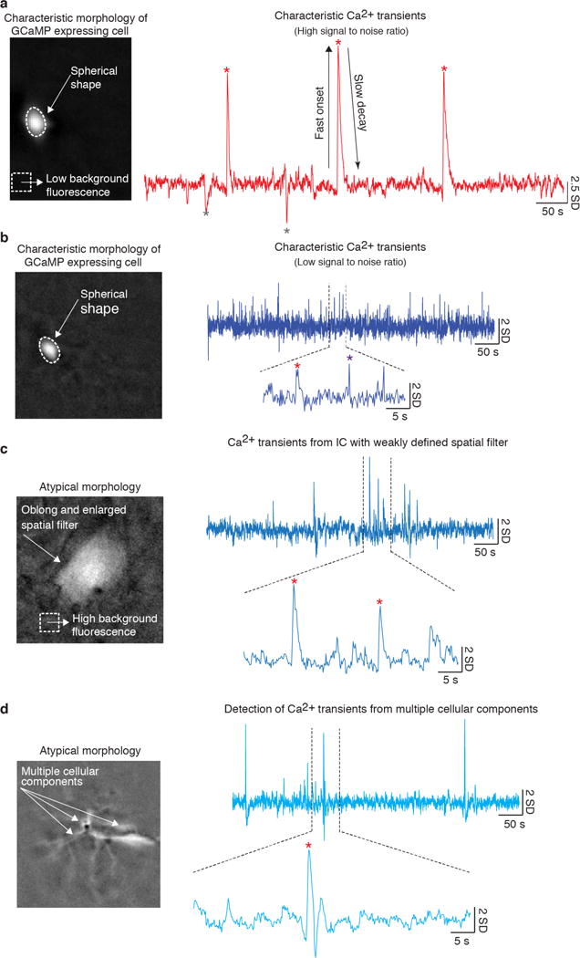
(a–d) Signals extracted via automated cell sorting algorithms will vary in data quality. In the examples shown here, cellular signals are ordered from (a) highest to (d) lowest quality and were extracted from digitally acquired Ca²⁺ imaging data using PCA/ICA analysis (Mosaic analysis software, Inscopix). This automated cell sorting algorithm deconstructs the data set into statistically independent signals (Independent components) composed of a spatial filter that indicates the number and coordinates of pixels that contribute to an identified signal (left) as well as an activity trace which shows how the intensity of pixels within this defined spatial filter change over time (right). (a) Independent components (ICs) that have the characteristics of dynamic fluorescence emissions from a GCaMP expressing cell should have a spatial filter with morphological features of a cell body (i.e., a spherical shape) as well as a an activity trace that resembles the temporal dynamics of a Ca²⁺ transient (i.e., a fast rise time and slow offset). This IC also has relatively low levels of background fluorescence compared to the large changes in signal fluctuation that occur during the three Ca²⁺ events (red stars) shown in the activity trace, indicating a high signal to noise ratio. Negative fluctuations in fluorescence emissions can also be seen within this activity trace (gray stars). While it is tempting to assign negative fluctuations in fluorescence intensity to decreases in neural activity for the identified cell, it is possible that decreases in fluorescence intensity arise from reductions in activity within the surrounding neuropil. Thus, decreases in cellular activity should be interpreted with caution when attempting to assign a specific physiological function²⁶. Nonetheless, the spatial and temporal characteristics of this IC strongly suggest that this signal is associated with dynamic Ca²⁺ activity of an individual cell. (b) Example of an IC with a lower signal to noise ratio than the example shown in a. The spatial filter shows morphological characteristics of a GCaMP expressing cell; however, the activity trace shows a mixture of peaks resembling those of temporal Ca²⁺ dynamics (red star), while others have non-representative characteristics (purple star). The inclusion of ICs with low signal to noise ratio should be conducted with caution. Although this IC likely represents neural activity of a single cell, possibly with low activity levels, it may also be a partial component of a cellular signal or a noise artifact. (c) Example of an IC with morphological characteristics that weakly resembles a GCaMP expressing cell (i.e., identified boundaries are not well defined). There is also a relatively high level of background fluorescence associated with this IC. Possible reasons for this weakly defined spatial filter may be that the IC represents an out of focus cell or possibly a cell whose shape has been optically distorted by the lens. Although the spatial filter of this IC is vaguely representative of a GCaMP expressing cell, the activity trace shows temporal dynamics characteristic of Ca²⁺ transients. However, due to the weakly defined spatial filter, it would not be recommended that this signal is included for analysis. (d) It is possible that cellular components with highly correlated signals may be extracted as one independent signal. For example, the spatial filter shown here has morphological features resembling those of dendrites, possibly from more than one cell, and the corresponding activity trace has fluctuations in signal intensity resembling dynamic Ca²⁺ activity. Given that the spatial filter cannot be localized to one cellular component, it is not recommended that this IC would be retained for future analysis. Data shown here was collected over one imaging session from adult male mouse expressing GCaMP6m (AAV-DJ-CamkIIa-GCaMP6m, Titer: 7.0 × 10¹², 1:1 dilution, Stanford) within the dentate gyrus. A 1 mm diameter lens was used to visualize cellular activity. All procedures were approved by UNC IACUC.

Given that the intensity of Ca²⁺ encoded signals can change as a function of time, it is important to consider both the duration of an individual recording session⁴² as well as how long a chronic imaging paradigm will be carried out for²⁹. More specifically, during an acute imaging session of particularly long duration (i.e., greater than 40-mins), it is possible for photobleaching of the signal to occur, resulting in a reduction in fluorescence intensity and or a reduction in the total number of detected cells to decrease throughout the recording sessions. If signs of photobleaching are apparent, the experimental design should be modified to either reduce the total duration of an imaging session or modified so that imaging data is only collected at experimentally relevant time points. For example, for pharmacological manipulations a 45-min imaging regimen can be used with 10-minutes intervals of the LED on followed by a 5-min off period for a total of 30-minutes of imaging data⁴². The inclusion off LED-off periods into a relatively long imaging session will reduce the risk of photobleaching.

As described above, chronic imaging paradigms have an additional level of complexity as steady increases in the expression of the Ca²⁺ indicator over time can result in both an increase in the fluorescence intensity of individual cells as well as the number of detected cells cross sessions. During the experimental procedure, basal fluorescence intensity should be monitored to confirm that fluorescence emissions are stable throughout the duration of the experiment²⁹. In addition to steady increases in fluorescence intensity, long-term expression of GCaMP may alter a cells natural ability to buffer Ca²⁺ and therefore alter neural activity and/or behavior. To confirm that an observed change in neural activity is the result of a particular experimental manipulation and not merely due to the expression of GCaMP within a defined neural population, a control group that is imaged at similar time points as the test group, but does not undergo any other experimental manipulations can be included (e.g., Surgery positive/GCaMP positive/Manipulation negative). Within the control group, neural activity should be stable throughout the duration of the test procedure. To confirm that the expression of GCaMP does not interfere with the performance of a behavioral task, the behavior of test subjects should be stable across time or change in a manner that is predicted by the behavior of animals that have undergone similar experimental procedures, but do not express GCaMP (e.g., Surgery positive/GCaMP negative/Manipulation positive)⁴². Alternatively, this experimental group could express YFP within the target neuron population so that motion induced changes in fluorescent intensity as well as GCaMP-induced changes in behavior can be controlled for in one group (e.g., Surgery positive/YFP-positive/Manipulation positive)³⁵. Finally, experimental subjects can also be monitored for gross changes in behavior or general indicators of health⁴².

The experimental controls and precautions listed in this section are recommendations primarily based on the experience of our laboratory with this methodology. Given the broad applicability of this technique to the field of neuroscience, these recommendations are unlikely to be a complete list. Thus, the appropriate experimental controls necessary for accurate data interpretation should be carefully considered before the start of an experiment. It is also important to consider if a freely behaving design is the ideal method to answer the experimental question. For instance, while a freely behaving design may be appropriate for complex behavioral tasks that require an animal to be able to move naturally through its environment and appropriately adapt its behavior to a dynamically changing stimulus, such as during species-typical social behavior, it may not be ideal for experimental questions that require precise time-locked exposure to an environmental stimulus, such as studies related to sensory processing. For the latter experiment, if the goal is conduct Ca²⁺ imaging within a deep brain neuronal structure, similar procedures for the introduction of GCaMP as well as the chronic implantation of a micorendoscope may be used as described in this protocol (Procedural steps 1–47) and subsequently combined with head fixed imaging procedures^20,44.

MATERIALS

Reagents

• Mouse line of choice (wild type, Cre line for targeting specific cell types, or transgenic mouse lines expressing GCaMP in a stable and uniform manner across cells for up to 6 months⁶¹ (available from the The Jackson Laboratory, www.jax.org).

  CAUTION Use of animal species should be conducted in accordance with institutional guidelines and regulations. UNC IACUC approved the procedures used in this protocol.

• AAV constructs (see Table 1 for a list of available viral constructs) Our laboratory has successfully utilized GCaMP6 viruses available from the University of Pennsylvania, Stanford University, and the University of North Carolina (UNC) Vector Core. The data shown in the present paper is from viral constructs created at Stanford and UNC. Other groups have successfully utilized variants of GCaMP available from the University of Pennsylvania Vector Core with similar imaging procedures described in this protocol^42,65. CAUTION Use and disposal of AAV constructs should be conducted in accordance with institutional guidelines CRITICAL For long-term imaging studies, an alternative to viral delivery of GCaMP is to use transgenic mouse lines that stably express GCaMP.

• Kwik-Sil adhesive (World Precision Instruments, cat. no. KWIK-SIL)

• Kwik-Cast sealant (World Precision Instruments, cat. no. KWIK-CAST)

• Mixer tips (World Precision Instruments, cat. no. 600009)

• Super glue liquid professional (Loctite)

• C&B-Metabond (Parkell, cat. no. S380)

• Absolute Ethanol – 200 proof (Fisher Bioreagents, cat. no. BP2818-4)

• Isopropanol, 70% v/v (Fisher Chemical, cat. no. A459-1)

• Jet denture repair powder (Lang Dental, cat. no. 1250)

• Ortho-jet crystal liquid fast curing acrylic resin (Lang Dental, cat. no. 0206; for pink dental cement)

• Contemporary ortho-jet liquid (Lang Dental, cat. no. 1506 Black; for black dental cement)

• Acrylic primer (Lang Dental, cat. no. 1602)

• Isoflurane CAUTION Gas anesthesia should be used in a well ventilated room⁶⁶

• Medical grade oxygen (Airgas, cat. no. OX USP125)

• Topical anesthetic (Lidociane, USP (Akorn, NDC: 17478-711-30)

• Tissue adhesive (Vetbond, 3M, cat. no. 1469SB)

• Eye ointment (Henry Schein, cat. no. 18582)

• 0.9% sodium chloride injection (Hospira, cat. no. 4888-20)

• Betadine solution, poviderm medical scrub (Butler Schein, cat. no. 003659)

• Ibuprofen, 160 mg/5 ml (Tylenol, Childrens Tylenol)

Table 1.

Viral constructs for the introduction of a Ca²⁺ indicator into the brain

Ca2+ Sensors	Stereotypes	Variants	Target	Vendor	Website
AAV.CAG.GCaMP6.WPRE.SV40	AAV1, AAV5, AAV9, pAAV	slow, medium, fast	Ubiquitous	Penn	http://www.med.upenn.edu/gtp/vectorcore/user_documents/DB_Catalog_040715.pdf
AAV.Syn.GCaMP6.WPRE.SV40	AAV1, AAV5, AAV9. pAAV	slow, medium, fast	Neurons	Penn	http://www.med.upenn.edu/gtp/vectorcore/user_documents/DB_Catalog_040715.pdf
AAV.CaMKII.GCAMP6.WPRE.SV40	AAV1, AAV5, AAV9	slow, medium, fast	Pyramidal neurons	Penn	http://www.med.upenn.edu/gtp/vectorcore/user_documents/DB_Catalog_040715.pdf
AAV.CaMKII.GCAMP6.WPRE.hGH	AAV1	fast	Pyramidal neurons	Penn	http://www.med.upenn.edu/gtp/vectorcore/user_documents/DB_Catalog_040715.pdf
AAV.GfaABC1D.cytoGCaMP6.SV40	AAV5	fast	Glia	Penn	http://www.med.upenn.edu/gtp/vectorcore/user_documents/DB_Catalog_040715.pdf
Cre-inducible Ca2+ Sensors	Stereotypes	Variants	Target	Vendor	Website
AAV.CAG.Flex.GCaMP6	AAV1, AAV5, AAV9	slow, medium, fast	Ubiquitous, Cre inducible	Penn	http://www.med.upenn.edu/gtp/vectorcore/user_documents/DB_Catalog_040715.pdf
AAV.Syn.Flex.GCaMP6	AAV1, AAV5, AAV9	slow, medium, fast	Neurons, Cre inducible	Penn	http://www.med.upenn.edu/gtp/vectorcore/user_documents/DB_Catalog_040715.pdf

Equipment

Surgery consumables

• Ideal micro drill bur, 0.8 mm (Cell Point Scientific, cat. no. 60-1000)

• Trephine for Microdrill (Fine Science Tools, cat. no. 18004-18)

• Stainless steel disposable scalpels (Miltex, cat. no. 4-410)

• 5-0 Sofsilk sutures (Covidien, cat. no. D4G1516X)

• 1 mL syringe (BD, cat. no. 309659)

• 27G 0.5-inch blunt needle (SAI Infusion Technologies, B27-50)

• 27G 0.5-inch needle (BD, cat. no. 305109)

• 25G 5/8-inch needle (BD, cat. no. 305122)

• 18G 1-inch needle (BD, cat. no. 305195)

• 18G 1.5-inch blunt needle (BD, cat. no. 305180)

• Dust-off compressed gas (Falcon Safety Products, DPSXL)

• Gelfoam absorbable sponge (Pfizer Injectables, cat. no. 00009-0342-01)

• 12-well culture plates (Falcon, cat. no. 353043)

• Skull screws (Glass and Watch Screws, 900 piece set, JT69900)

• 1/16-inch diameter heat shrink tubing (Qualtek, cat. no. Q2-F3X-1/16-01-MS100FT)

• Carbon filter (ReFresh, cat. no. EZ-258)

• Parafilm (Parafilm, PM-999)

Optical materials

• Microendoscopic lens (see Table 2 for options available from Inscopix,)

• Microscope baseplate (Inscopix, cat. no. BPL-2)

• Microscope baseplate cover (i.e., dust cap) (Inscopix, cat. no. BPC-2)

• Microscope Gripper tool (Inscopix, cat. no. GRP-1)

• Hex key (Inscopix, cat. no. ATW-1)

• Dummy microscope (Inscopix, cat. no. DMS-2)

• Microscope objective lens cover (Inscopix, cat. no. MSC-2)

• Optical Cleaning Kit (Fine Science Tools, cat. no. 29000-10)

• Premium grade lens cleaner (Thorlabs, cat. no. MC-50E)

• *Methods in this protocol have been developed and tested using optical materials purchased from Inscopix. For other imaging system and microendocopic lens options please see the following websites (doriclenses.com, welcome.gofoton.com).

Table 2.

Commercially available microendoscopes (from Inscopix)

Name	Part ID	Diameter	Length	Working Distance Object (Water)	Working Distance Image (Air)
Lens probe 1040	GLP-1040	1.0 mm	4.0 mm	~290 um	~60 um
Lens probe 0673	GLP-0673	0.6 mm	7.3 mm	~290 um	~230 um
Lens probe 0561	GLP-0561	0.5 mm	6.1 mm	~290 um	~230 um
Lens probe 0584	GLP-0584	0.5 mm	8.4 mm	~290 um	~230 um
Lens probe 0540	GLP-0540	0.5 mm	4.0 mm

Surgery tools and equipment

• Vannas spring scissors (Fine Science Tools, cat. no. 15000-08)

• Curved graefe forceps (Fine Science Tools, cat. no. 11052-10)

• Dumont 7 ceramic coated forceps (Fine Science Tools, cat. no. 11272-50)

• Dumont 5 forceps (Fine Science Tools, cat. no. 11251-10)

• Dissecting chisel (Fine Science Tools, cat. no. 10095-12)

• Curved 50 mm bulldog clamp (Fine Science Tools, cat. no. 18051-51)

• Bonn micro probe (Fine Science Tools, cat. no. 10033-13)

• Micro curette (Fine Science Tools, 10082-15)

• Bulldog serrefine (Fine Science Tools, cat. no. 18050-28)

• Glass bead sterilizer (Simon Keller, cat. no. Steri 250)

• Pump 11 Elite (Harvard Apparatus, cat. no. 70-4505)

• 7002KH 2.0 uL syringe (Hamilton, cat. no. 88400)

• Modular Routine Stereo Microscope with 8:1 Zoom (Leica, cat. no. M80)

• Model 942 Small Animal Stereotaxic Instrument with Digital Display Console (Kopf, cat. no. 942)

• Non-rupture Mouse Earbar (Kopf, cat. ID. Set 2, Model 922)

• Electrode holder with removable open side clamp (Kopf, Model 1773)

• Cannula holder (Kopf, Model 1776-P1)

• Microdrill (Cell Point Scientific, cat. no. RS-67-1000)

• Stereotaxic handpiece holder (Kopf, Model 1466-B)

• Precision screwdriver (Westward, cat. no. 1UG41)

• Homeothermic monitor (Harvard Apparatus, cat. no. 50-7220-F; for surgery)

• Animal anesthesia kit (E-Z Anesthesia, cat. no. EZ-7000)

• Oxygen regulator (E-Z Anesthesia, cat. no. EZ-320)

• Heating pad (Sunbeam, cat. no. 126982; for recovery)

• Heat gun (Weller, cat. no. 6966C)

• Fixed Sliding Probe Carriage (Scientifica, cat. no. PS-7750)

• Patchstar Micromanipulator (Scientifica, cat. no. PS07000C)

• ½″ Articulated ball and socket mount (Thor labs, TRB1)

In vivo imaging equipment and data analysis

• SPRO ball bearing swivels with interlock snap (Cabelas, IK-117351)

• Model 923-B Mouse Gas Anesthesia Head Holder (Kopf)

• Arduino circuit board (Arduino, cat. no. A000066)

• Bayonet Neil-Concelman Connector (BNC) (f) with American wire gauge (AWG) leads (Ponoma Electronics, cat. no. 4969)

• Desktop with Intel core i7 processor, Windows 8.1, ideally with 32GB of memory (eg. Lenovo, K450 Ideacenter; for data analysis) <m>CRITICAL</m> In vivo Ca²⁺ imaging sessions create large datasets and it is recommended that a computer for the analysis of these data sets with specifications of at least an Intel core i7 processor, 8 GB of RAM, 2 terabyte free hard disk space, and USB 3.0 ports.

• Desktop with Intel core i5 processor, Windows 8.1, and at least 8GB of memory (eg. Dell, XPS8700; for data acquisition)

Reagent Setup

• Virus preparation: Prior to stereotactic injection of the virus, if necessary, dilute the virus with sterile saline. Recommended virus dilutions are as follows: 1:2, 1:4, 1:8, 1:16, and 1:32. If the virus is being used that day, store on ice until it is time to conduct the virus infusion procedure. Store all remaining aliquots at −80° Celsius. Under conditions of minimal freeze/thaw cycles, virus aliquots can typically be stored for ~5 years.

• Pink dental cement (for the foundation of the head cap): Prior to the start of the surgery, fill each well of a 12-well plate with 2 g of acrylic powder. When ready to secure the microendoscope to the skull, mix 1 mL of clear Ortho-Jet liquid with the powder located in one well and load the mixture into a 1 ml syringe. Attach an 18G 1.5-inch blunt needle to the filled syringe. Wait at least 30 seconds before applying the dental acrylic solution to skull. CRITICAL Prepare well plates with dental cement before beginning surgical procedures for the implantation of a microendoscope.

• Black dental cement (blocking background light and the attachment of the baseplate): prepare a well plate with acrylic powder as described above. When ready to apply the black dental cement to the head cap or baseplate, add 1 ml of black Ortho-Jet liquid to the powder and load the mixture into a syringe as described above. Wait ~30 seconds before applying to the skull. CRITICAL Prepare well plates with dental cement before beginning surgical procedures for the attachment of the baseplate.

• Ibuprofen for post-operative care: Fill the water bottle that is to be placed in the test subject’s home cage with 200 mL of water and add 2.5 ml of Childrens Tylenol (80 mg ibuprofen/200 mL water). Allow water bottle to remain in home cage for 2–3 days.

• Post-operative recovery cage: Prior to the start of surgical procedures, it is recommended that a clean cage (fresh bedding, softened chow, nestlet material, and a paper towel for the animal to be placed on immediately post-operatively) be prepared for the test subject to recover in. If a wire lid is used to hold chow, it is recommended that this is removed to reduce the number of physical objects in the cage that can potentially cause damage to the exposed surface of the lens. This analgesia and recovery procedure has been approved by UNC IACUC and should be conducted in accordance with the guidelines of your institution.

Equipment Setup

• Heat shrink covered surgery tools: When handling delicate optical materials, such as the microendoscope, apply heat shrink tubing to hard metal tools. For general lens handling, apply heat shrink to the Dumont 5 forceps, with ~10 mm of tubing added to each arm. Cut heat shrink to appropriate size and fix the heat shrink to the forceps with the application of the heat gun (Supplemental Fig 1a).

• Lens holder: Cut two 5-mm long heat shrink sleeves. Slide heat shrink over each arm of the bulldog serrefine and apply heat with heat gun (Supplemental Fig 1b). When it is time to implant the microendoscope, clamp the back end of the serrefine in the cannula holder (Supplemental Fig 1c) and mount the entire apparatus on the stereotax (Supplemental Fig 1d). Next, secure the microendoscope into the heat shrink covered arms of the bulldog the serrefine. When the lens holder has been secured to the stereotax, visually inspect the microendoscopic lens to ensure that it is leveled within the clamp. Once the microendoscope is leveled, it is ready to be lowered into the brain. CRITICAL It is recommended that all lens handling procedures are conducted over lens cloth to prevent damage to the lens in the case that it is accidently dropped during the preparation stage.

• Bent needle for bone extraction: Using curved graefe forceps, bend the tip of a 27G 0.5-inch needle ~45 degrees (Supplemental Fig 1e).

• Sterile saline for irrigation during surgery: Attach an 18G 1-inch needle to a 1 ml syringe and fill with sterile saline. Use this syringe to apply sterile saline throughout the craniotomy and lens implantation procedure.

PROCEDURE

Virus Dilution Study

CRITICAL If using transgenic mice expressing GCaMP in a stable and uniform manner across cells, this section is not necessary and you can proceed direct to step 5.

• 1Before beginning in vivo imaging experiments, select the appropriate variant of GCaMP (fast (f), medium (m), slow (s)) and optimize the concentration of virus for the neuron population by first conducting a virus dilution study. Inject various dilutions of the desired viral construct into the brain region and mouse line of interest. Perform previously described stereotaxic procedures to introduce the viral construct into the brain (Fig 4a)

  CRITICAL STEP Variants of the ultrasensitive GCaMP6 Ca²⁺ sensors outperform other sensors in vivo, but still warrant consideration of temporal precision during live imaging and post processing. These indicators vary in kinetic properties and sensitivity, with sensors with slower kinetics having greater sensitivity. For example, GCaMP6f and GCaMP6m have faster kinetics (determined by the rise time + half the decay time) compared to GCaMP6s and thus a greater potential to separate individual spikes within a burst or detect single action potentials in neuronal populations that exhibit fast firing rates. However, due to the fast binding kinetics of these variants, GCaMP6f and m have lower signal intensities during excitatory events that are associated with a low number of action potentials¹⁴. Thus, selection of variant will depend on the firing rate and signal to noise ratio of the cell population being imaged.

  TROUBLE SHOOTING

• 2Methods for virus introduction used in this procedural step, such as microinjections with a Hamilton syringe or Nanoject, should be similar to those planned to be used in experimental subjects. Recommended virus dilution concentrations to test are 1:2, 1:4, 1:8, 1:16, and 1:32 of virus diluted from a high titer viral stock. Allow at least 3 weeks for sufficient viral expression to occur (Fig 4b).

  TROUBLE SHOOTING

• 3When sufficient time has elapsed for viral expression of the Ca²⁺ indicator, perfuse the subject as described in references 67 and 68 and examine the proportion of cells expressing GCaMP as well as the health of GCaMP expressing cells (Fig 4c–e)^67,68. Healthy cells should show nuclear exclusion of GCaMP6, exhibiting a honeycomb shaped appearance (Fig 5 a,b, Supplemental video 1). If GCaMP6 expression is observed throughout the entire cell body, resulting in a complete filling of the cell body with the fluorescence indicator, it is likely that over expression of the Ca²⁺ indicator has occurred leading to unhealthy cells and, eventually, cell death (Fig 5a). CRITICAL STEP Completion of this step prior to conducting imaging experiments is critical as different AAV serotypes or promoters may not be optimal for all cell types^69–71 (see Table 1 for a list of available viral constructs). CRITICAL STEP Optimal viral transduction is dependent on viral titers as well as the efficiency of a particular virus for transducing a given cell type. Caution should be taken when directly comparing viral titers between vector cores as quality control assays and methods for determining physical and infectious titer can vary. Physical titer is expressed as the number of virus particles, viral genome, or genome copies per unit of measurement. Functional or infectious titer is the measure of virus that infects a target cell. This is expressed as transduction units per mL or plaque forming units per mL. These values are not absolute, but rather a relative measure of infectivity and direct quantitative measurements are therefore not comparable across vector cores.

  TROUBLE SHOOTING

• 4If your experimental paradigm requires chronic imaging sessions (i.e., weeks to months) repeat steps 1 and 2 with suitable viral dilutions and examine viral expression at the longest time point planned for the experiment (e.g. 8 – 12 weeks after virus injection). It is particularly critical that cell health is examined at these later time points to ensure that long-term expression of GCaMP does not result in cell death. Cell health can be examined after the completion of an experiment by examining mounted tissue sections under a microscope (i.e., post tissue histology)^24,25 (Fig 5a) or with 1- or 2-photon microscopy in living mice (awake or anesthetized) throughout the experiment²⁹ (Fig 5b). Post tissue histology is recommended for the initial optimization of virus dilution, while 1- or 2-photon microscopy is best suited to confirm stable GCaMP expression and neural activity during the experiment. CRITICAL STEP It is normal for virus expression levels of GCaMP to increase stably, and, moderately over time, resulting in greater changes in fluorescence intensities compared to those measured at earlier time points as well as an increase in the proportion of cells that express GCaMP^17,27. Thus, it is critical that stable virus expression throughout the duration of the study is optimized prior to the start of in vivo imaging experiments to ensure accurate data interpretation.
• 5If targeting a genetically defined population of neurons, confirm cell type specific expression using immunohistological methods (for example, Supplemental Fig 2a–d).

Figure 4. Conduct virus dilution study.

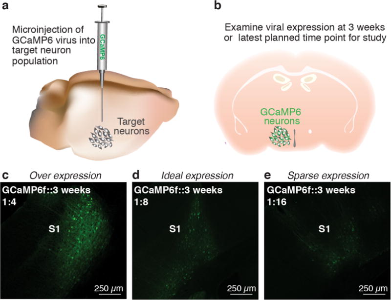
(a) Microinject GCaMP6 virus into target neuron population. (b) Allow the virus to express for at least 3 weeks before examining expression level of indicator. (c-e) Confocal images showing GCaMP6f expression within the somatosensory (S1) cortex of a wild-type mouse (DIO-GCaMP6f; Titer: 3.9 × 10¹², UNC vector core). (c) 1:4 dilution shows overexpression of GCaMP6f in cortical neurons as indicated by cells that lack a honeycomb appearance. (d) 1:8 dilution shows ideal expression of GCaMP6f as there is a relatively large amount of healthy looking cells expressing the GCaMP6f virus. (e) 1:16 dilution shows sparse expression of GCaMP6f. Ca²⁺ signals from such expression will be more difficult to detect compared to the 1:8 dilution and yield low cell count.

Figure 5. Example of healthy and unhealthy GCaMP expression.

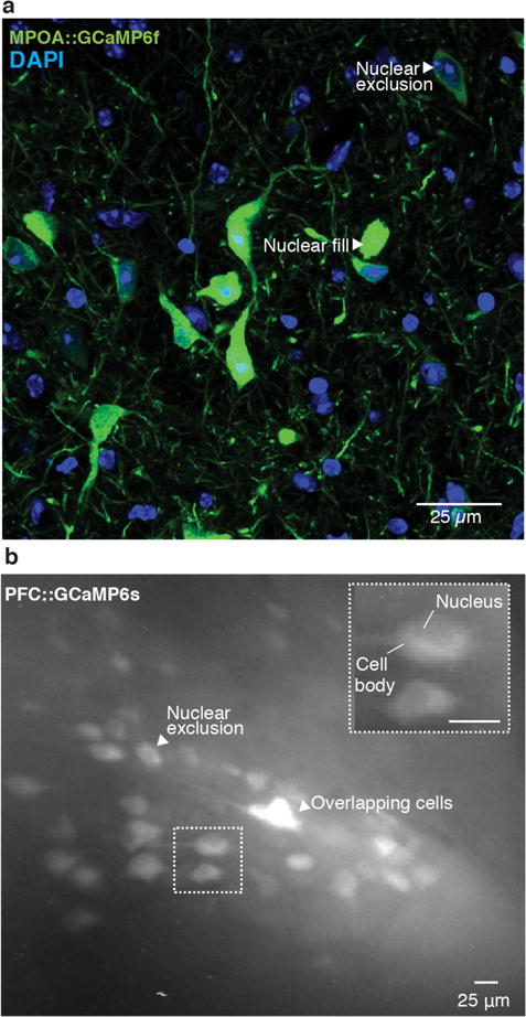
(a) Neurotensin-Cre adult female mice were injected with a 1:1 dilution of DIO-GCaMP6f (Titer: 3.9 × 10¹², UNC vector core) into the medial preoptic area (MPOA) and perfused 4 weeks post injection. 40× confocal image depicts expression levels of GCaMP6f in MPOA neurotensin neurons. Arrows indicate cells showing nuclear exclusion of GCaMP6f (healthy expression) as well as nuclear filling (unhealthy expression). Due to a relatively large number of cells showing nuclear filling of GCaMP at only 4 weeks, this dilution would not be recommended for this cell population. (b) Optical detection of healthy GCaMP expressing neurons within the prefrontal cortex (PFC) of a freely behaving WT mouse. PFC neurons were visualized through a 1 mm diameter GRIN lens with a head-mounted, miniature microscope secured to the skull of the mouse. The recording was conducted 8 weeks following virus injection (AAV-DJ-CamkIIa-GCaMP6s, 5.3 × 10¹², 1:6 dilution, UNC vector core) and lens implantation over a 10-min session. A maximum intensity projection was made of the entire 10-min recording session to facilitate the visualization of optically detected neurons. In this image, neurons with dark centers can be visualized, indicating a lack of nuclear filling and that optically detected cells are healthy. All procedures were approved by UNC IACUC.

Selection of microendoscopic lens

• 6
  Select the appropriate lens for your brain region of interest (see Table 2 and Fig 6a). The lens should be long enough to reach just above your neuronal population of interest, while still allowing for ~2 mm of the lens to protrude above the skull (Fig 6b). When selecting the appropriate microendoscope for your neuron population, it is also important to weigh the optical properties of the microendocope with the invasive nature of the lens implantation procedure. For example, both the transmission of light to and from the brain as well as field of view size increase with lens diameter, optical properties which both impact signal detection capabilities (Supplemental Fig 3a,b). However, as lens diameter increases, so does the extent of tissue damage. Thus, the length and diameter of lens selected should be optimized to visualize the neuron population of interest, while minimizing damage to the underlying neural tissue.

  • CRITICAL STEP Before beginning surgeries on experimental subjects, it is beneficial to optimize the placement of the microendoscope in relation to the target neuron population. For the lenses utilized in this protocol, the focal plane is ~290 μm below the surface of the lower lens. Thus, to bring neuronal signals into focus, the bottom of the microendoscope should sit between 200 and 300 μm above GCaMP expressing neurons (Fig 6c). Given this relatively narrow range in the dorsal-ventral imaging plane, it is highly recommended that the viral indicator is also injected during the lens optimization procedure. During post-histology, the distance between the bottom of the lens and GCaMP expressing neurons can be calculated to validate the appropriate placement of the lens (Fig 6c). Optimizing these steps prior to beginning a large cohort of animals will decrease the number of subjects in which the focal plane of the lens is out of range of the target cell population (Fig 6d).

  TROUBLE SHOOTING

Figure 6. Selection of microendoscopic lens and optimization of surgical placement.

(a) Cartoon diagram of microendoscopic lens (Relay lens bound at either end by a GRIN lens) designed to transmit light below the surface of the brain. (b) Microendoscopic lenses of varying length and diameter are available for chronic brain implantation. Wide diameter lenses (e.g., 1 mm) can transmit more light to and from the brain than lenses with narrow diameters (e.g., 0.5 and 0.6 mm), but the increased surface area of these lenses also results in more tissue damage. Thus, 1mm diameter lenses are best suited for more superficial regions of the brain, while 0.5 mm lens that produce comparatively less pressure on underlying tissue are better suited for deep brain regions. When selecting the appropriate microendoscopic lens, it is important to keep in mind that the total length of the lens must be sufficient to reach the target neuron population while still allowing for at least 2 mm of the lens to extend above the skull to accommodate dental cement application. (c) 10× confocal image showing an example of a correctly placed lens relative to the target neuron population. (d) 20× confocal image showing a lens that was placed medial to the target neuron population, resulting in a lack of GCaMP6 expressing neurons in the focal plane of the lens. For c and d, the tract for the microendoscopic lens is outlined in yellow, and the location of the focal plane is, ~290 μm below the bottom of the lens, outlined in orange. Tissue shown in both images was counterstained for DAPI (nuclear stain). All procedures were approved by UNC IACUC. Panels adapted from Jennings et al., 2015.

Surgical preparation for craniotomy and lens implantation

CRITICAL Once the virus dilution has been optimized and the appropriate microendoscope has been selected, lens implantation surgery can be begun on experimental subjects.

• 7Prior to beginning surgical procedures, anesthetize the animal with isoflurane. Gas anesthesia is preferred over an injectable anesthesia, such as the combined use of Ketamine and xylazine, due to the long duration of the surgery⁶⁶.
• 8Next, stabilize the mouse’s head in the stereotaxic apparatus⁷² (Fig 7a).
• 9Perform aseptic procedures in accordance with the guidelines of your institution. We perform surgical procedures in a designated, sanitized area (Fig 7a), autoclave all instruments, pluck hair from the surgical site (Fig 7b), and clean the surgical site with 3 alternating scrubs of isopropyl alcohol and betadine (Fig 7c).
• 10To reduce the perception of pain at the surgical site and therefore lower the level of general anesthetic needed to maintain anesthesia during surgery, we recommend application of topical lidocaine to the procedure site.
• 11Make a small incision (~12 to 15 mm) along the sagittal line of the skull by using graefe forceps to hold the skin taught while running a scalpel blade in a straight line from the anterior to posterior region of the exposed skin. Use 4 curved 50 mm bulldog clamps to further expose the skull (Fig 7d). If necessary, use Vanna spring scissors to cut a larger opening in the skin and remove any hair that may be too close to the area of the skull where the head cap will be made.
• 12To increase the accuracy of stereotaxic procedures, ensure that the skull is level by comparing the height of bregma in relation to lambda (Fig 7e). The difference in height between lambda and bregma should be less than 0.05 mm (Fig 7f,g). If the difference in height between the two is greater than 0.05 mm adjust the position of the skull in the dorsal-ventral direction until it is leveled. Next ensure that the skull is level in the medial-lateral direction by measuring the height of the skull at a set distance posterior from bregma, such as −2.0 mm, and an equal distance lateral from the midline on either side of the skull, such as ± 1.5 mm (Fig 7h). The difference in height at each location from the midline should also be less than 0.05 mm in the dorsal ventral direction. If the difference is greater than 0.05 mm, rotate the mouse’s skull using the bite bar or reposition the mouse’s head in the ear bar⁷².

  TROUBLE SHOOTING

• 13To reduce the occurrence of movement noise during in vivo imaging sessions, remove connective tissue from the top of the skull and muscle near the top edge of the skulls surface. Use a cotton tip applicator to remove periosteum and connective tissue from the skulls surface (Fig 8a). Use the dissecting chisel to clear away all tendons and muscles located near the area of the skull where the head cap will be made⁷³ (Fig 8b). Apply sterile saline to the skull once all connective tissue has been removed. CRITICAL STEP It is crucial that connective tissue, tendons, muscle, skin, or fur are not allowed to come in contact with the dental cement that will be used to form the head cap (Fig 8c). This can cause the head cap to become loose, increasing movement noise during recording sessions or possibly resulting in the loss of an experimental subject.

  TROUBLE SHOOTING

• 14Use the 0.8 mm burr to drill holes for the placement of three skull screws (Fig 9a). When drilling is complete, use an air can and a cotton-tip applicator to clear away any debris from the skull (Fig 9a). To reduce the likelihood of excess bone fragments getting into the craniotomy site, we recommend that the drilling of skull screw holes and the removal of bone debris from this procedure occur before the craniotomy is performed. CRITICAL STEP For maximum stability of the microendoscopic lens, each screw should be equally placed in a triangle shape about 1.5 cm from the craniotomy site (Fig 9a).
• 15Irrigate the skull with sterile saline to reduce tissue over heating during the craniotomy procedure (Fig 9b).

Figure 7. Surgery preparation for virus injection and microendoscopic lens implantation.

(a) Stabilize mouse in stereotaxic apparatus. (b) Use forceps to pluck hair from the top of the skull. Digital image below shows example of how the skin should appear after a significant amount of fur has been plucked. (c) Perform alternating alcohol and betadine scrubs (3×). Digital image below shows example of the area of the skin where alcohol and betadine should be applied. Betadine (brown liquid) is shown here. (d) Open the skin with a scalpel and bulldog clamps. Digital image below shows example of the size of the opening that should be made as well as appropriate placement of the bulldog serrafine. (e) Cartoon image showing location of bregma and lambda on mouse skull. (f and g) Center the drill bit on (f) bregma and (g) lambda for leveling the skull. The distance in the z-plane between the two locations should be less than 0.05 mm. (h) Level the skull in the medial-lateral direction by moving the drill bit to −2.0 mm posterior from bregma, and measuring the difference in the z-plane between ±1.5 mm from the midline. The difference between the 2 points should be less than 0.05 mm. All procedures were approved by UNC IACUC.

Figure 8. Removal of connective tissue and muscle.

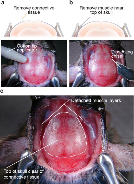
(a) To reduce movement noise during imaging sessions, remove connective tissue by rubbing a cotton tip applicator on the top surface of the skull. Digital image below shows example of skull in which connective tissue has been removed by gently rubbing a cotton tip applicator on the top of the surface. (b) To further reduce the likelihood of movement artifacts, use a dissecting chisel to cut away muscle and tendons making contact with the top edge of the skull. Digital image below shows specific area of the skull where the dissecting chisel should be used to remove muscle. (c) When finished, the surface of the skull should be clear of connective tissue and the muscle retracted from the portion of the skull where dental cement will be applied during the head cap procedure (dotted outline on skull). All procedures were approved by UNC IACUC.

Figure 9. Perform craniotomy.

(a) Before performing craniotomy, drill 3 holes for the placement of skull screws in a triangle shape around the future craniotomy site. Clear away debris created by the drilling procedure (inset) before further opening up the skull to reduce the likelihood of bone debris entering the craniotomy. (b) Irrigate the skull with sterile saline to prevent tissue overheating. (c) Center the trephine drill bit on bregma and manipulate the drill using the stereotaxic arm so that the center of the trephine is located above the stereotaxic coordinates where the lens will be implanted. (d) Slowly lower the running drill to outline the craniotomy. Continue to drill until only a thin layer of skull remains. (e) Close-up of craniotomy outline. (f) Use a bent 27 and ½ gauge needle to break away the remainder of the skull. Digital image below demonstrates where on the edge of the craniotomy the bent needle should be placed. (g) Once the center bone fragment is completely loose from the skull, carefully pull it away with a pair of fine tipped forceps. Zoomed in portion of g shows how the tissue under the fragment should appear. Notice that very little bleeding has occurred. (j) Irrigate the skull with sterile saline. All procedures were approved by UNC IACUC.

Craniotomy, durotomy, and tissue aspiration

• 16Prior to performing the craniotomy, attach the trephine drill bit to the microdrill and zero the center of the trephine drill bit above bregma (Fig 9c). Move the trephine drill bit to the x,y coordinates where the microendoscope will be implanted (determined by mouse atlas)⁷⁴.
• 17To etch away the skull, slowly lower the trephine drill bit up and down on the exposed skull (Fig 9d). Stop drilling when only a thin layer of skull remains (Fig 9e). A craniotomy may also be performed using a 0.8 mm drill bit to etch a cranial window that is just large enough to perform the virus injections (if necessary) as well as lower the microendoscope. A cranial window that is just large enough to implant the lens will stabilize the lens and minimize movement noise. CRITICAL STEP To prevent overheating, do not allow the drill bit to remain in one location for too long. Overheating the skull may result in bleeding under the skull.
• 18Use a bent 27G 1.5-inch needle (or Bonn microprobe) to break through the remaining skull and loosen the large skull fragment in the center of the craniotomy (Fig 9f).
• 19With Dumont 7 ceramic-coated forceps, grab onto the large skull fragment and move it away from the brain (Fig 9g).
• 20Immediately irrigate the exposed tissue with sterile saline (Fig 9h).
• 21Use a bent 27G 1.5-inch needle (or Micro curette) to remove any remaining small bone fragments.

  TROUBLE SHOOTING

• 22To facilitate virus injection and lens implantation, perform a durotomy (Fig 10a). Use the bent 27G needle (or Bonn Micro Probe) to pierce through the dura and slowly peel it away from the brain (Fig 10b). Compared to brain tissue, dura has a yellow tint to it (Fig 10b) and exposed neural tissue should appear white once the dura has been removed (Fig 10c). CRITICAL STEP When removing dura, be careful to avoid rupturing vasculature. If bleeding occurs during the procedure, pause the procedural step and apply a few drops of sterile saline to the exposed tissue. Use a pair of forceps to gently place a small piece of gel foam on top of the exposed tissue. Allow the saline-soaked gel foam to remain on the tissue until all bleeding has subsided. Once bleeding has stopped, use a pair of forceps to remove the gel foam and irrigate the area with sterile saline. CRITICAL STEP It is important that sterile saline is used in conjunction with the gel foam to prevent the gel foam from sticking to the tissue resulting in damage to the underlying tissue when the gel foam is removed.

  TROUBLE SHOOTING

• 23Irrigate the exposed brain tissue with sterile saline immediately following completion of the durotomy.
• 24Implantation of a microendoscopic lens deep within the brain will result in a large amount of pressure on the underlying neural tissue. To minimize tissue pressure, gently aspirate tissue above your region of interest (at least 1–2 mm of superficial layers for deep brain regions) (Fig 10d). Before beginning the aspiration, bend a blunt 27G needle 90° and connect the bent needle to a vacuum pump. Test the vacuum pressure by slowly approaching the saline bubble on top of the skull with the needle and adjust the pressure of the vacuum pump so that only a small volume of saline is aspirated at a time. To allow constant, fine control of suction pressure by hand, a 1 mm hole can be drilled into the plastic fitting of the needle providing an exhaust for redirection of airflow²⁰. Large changes in saline volume should not be immediately visible by eye. If large changes in volume are readily visible, the pressure of the pump should be lowered.

  TROUBLE SHOOTING

• 25
  To begin tissue aspiration, slowly lower the needle toward the exposed neural tissue while continuously applying sterile saline, aCSF, or Ringer’s solution for irrigation (Fig 10e). Some bleeding is normal during aspiration and adjustments in irrigation rates should be made to maintain tissue visibility as well as prevent the formation of large blood clots. This can be completed by stopping irrigation and aspiration for 5s intervals, allowing only small clot formation. Gel foam can be used to control bleeding at the edges of the aspiration site. Aspiration should stop when at least 1 mm of tissue has been aspirated or at least a thin layer of tissue (500–800 um) remains above your region of interest²³. We have found more conservative estimates of tissue aspiration (i.e., aspiration of 1–2 mm of tissue when implanting a probe 4 mm into brain) to sufficiently reduce tissue pressure, while minimizing the risk of damage to the target structure (Fig 10f).

  • For some brain regions, structural landmarks can be used to determine when the aspiration procedure should stop. For example, when aspirating tissue for the implantation of a microendoscopic lens in the hippocampus, aspiration should stop when the white matter tracts of the corpus callosum become visible (indicated by a shiny appearance to the tissue).
    We do not recommend that tissue is aspirated for superficial structures, such as the cortex.
    CRITICAL STEP To further minimize pressure-induced tissue damage, a needle can be lowered about 2.0–2.5 mm above the region of interest and subsequently retracted. This needle serves as a way to further clear a path for lens implantation and does not function to suction tissue from the brain.

  TROUBLE SHOOTING

Figure 10. Durotomy, tissue aspiration, and virus injection.

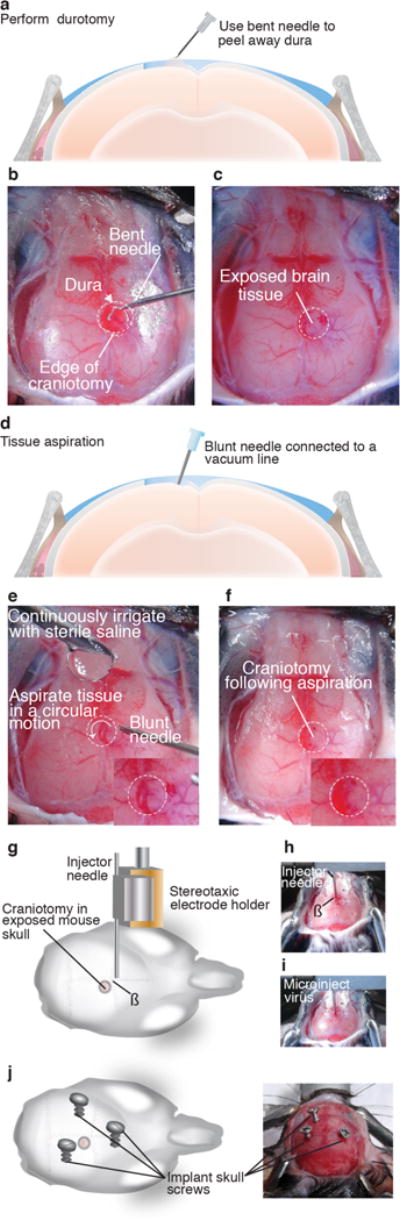
(a) Perform durotomy to facilitate virus injection and lens implantation. Remove dura matter from the surface of the brain using a bent 27 and ½ gauge needle. Hook dura on the tip of the needle and gently pull away from the brain. Continue to carefully pull away portions of the dura until a large enough opening is made for the injector needle and microendoscope to penetrate. (b) Example image showing thin layer of dura pulled away from brain tissue. (c) Image showing exposed brain tissue after completion of the durotomy. Brain tissue should appear white compared to dura matter (d) Aspirate tissue above target structure with a blunt needle connected to a vacuum pump (e) Aspirate in a circular motion while continually irrigating the tissue with sterile saline. Inset shows close-up of tissue prior to completion of aspiration procedure. (f) Exposed brain tissue after aspiration of 1 mm of tissue. Inset shows close-up of tissue after aspiration. (g) If viral injection is required for the expression of the Ca²⁺ indicator, load an injector needle containing the virus into stereotaxic electrode holder. (h) Center the injector needle on bregma and (i) based on stereotaxic coordinates for target neuron population, move guide cannula to region of interest and begin virus infusion. (j) When virus injection is complete, implant skull screws. All procedures were approved by UNC IACUC.

Introduction of Ca²⁺ indicator into neural population of interest

CRITICAL If the viral construct was injected at an earlier time point^42,75, or if a transgenic mouse line that expresses a Ca²⁺ indicator is being used (ww.jax.org), skip procedural steps 26 and 27 and proceed straight to step 28.

• 26Utilize established stereotaxic procedures to introduce the selected GCaMP encoding viral construct into the brain region of interest^27,46 (Fig 10g). To infuse virus in the mouse brain, our laboratory utilizes an injector needle connected to a 2 μl Hamilton syringe by PE20 tubing, but other methodologies for microinjections, such as with the use of a Nanoject, may also be used. Load the desired amount of viral construct (250–500 nL) into an injector needle and secure the injector needle onto the stereotaxic apparatus (Fig 10g). Center the injector needle above bregma and move the needle to the appropriate stereotaxic coordinates (Fig 10h,i). We recommend that the site of viral infusion be placed 250 μm medial/lateral and ventral to the site of lens implantation to minimize tissue damage under the lens (Supplemental Fig 4).

  TROUBLE SHOOTING

• 27
  Infuse virus at a constant, slow rate of 100 nL/min.

  • If imaging a vertical plane, such as with a prism lens that bends light at a 90° angle^77–79, multiple injections along the imaging plane may be required. For example, if imaging within cortical regions of the brain, it may be necessary to make at least three 250 nL injections spaced about 250–300 μm apart along the dorsal-ventral axis to successfully capture neural activity across multiple cortical layers. For 1.0 mm diameter lenses, multiple injections along the medial-lateral axis (e.g., ± 300–500 μm lateral from the center of the lens) may increase the amount of GCaMP expressing cells in the focal plane, but is not required for signal detection.

  TROUBLE SHOOTING

Lens implantation

• 28Before beginning lens implantation, implant the skull screws in the holes drilled in step 14 (Fig 10j). These screws will act to anchor the dental cement to the skull. The final placement of the skull screws should not protrude out of the skull at a point higher than the final height of the implanted lens. This height will depend on the length of the lens that is being used as well as the depth in which this lens is implanted in the brain.

  TROUBLE SHOOTING

• 29Attach the prepared lens holder to the stereotaxic apparatus (Supplemental Fig 1).
• 30Prepare the microendoscope for placement into the lens holder by gently placing the microendoscope on the lens cloth from the Optical Cleaning Kit. Using heat shrink covered Dumont 5 forceps, pick up the microendoscope and use an air can to gently remove any dust particles (Fig 11a). CRITICAL STEP The microendoscope is composed of two GRIN lenses attached onto either side of a relay lens. To avoid damaging either imaging surface, the microendoscope must be handled with care.
• 31Hold the microendoscope with heat shrink covered forceps in one hand and use the other hand to open the heat shrink covered bulldog serrefine clamp. Place the microendoscope in the bulldog serrefine clamp and carefully adjust the placement of the microendoscope in the holder until it is level within the apparatus (Fig 11b).
• 32Without touching the microendoscope to the skull, zero the microendoscope just above bregma and move the microendoscope to the target location.
• 33
  Before the lens is lowered, visually inspect the craniotomy site for bleeding. CRITCAL STEP It is crucial that all bleeding has stopped before the microendoscope is lowered as excessive bleeding may occlude the field of view.

  • If bleeding does occur at any stage of the procedure, apply gel foam to the craniotomy site until bleeding has subsided. If bleeding from the craniotomy site cannot be stopped, a lens should not be implanted as the bleeding will likely occlude the field of view under the lens.
• 34
  Carefully lower the lens to ~300 μm above the target neuron population. The microendoscope should be lowered at a constant, slow-rate, ~100–200 μm/min in steps of 10–20 μm (Fig 11c). The slower rate of 100 μm/min is recommended to achieve optimal recording conditions. Bleeding should not occur during this process and brain tissue as well as small vasculature should be visible under the lens throughout the duration of the lens implant procedure (Supplemental Fig 5). CRITICAL STEP Lowering the microendoscope at a slow rate may provide the neurons, glia, and vasculature time to separate, thus reducing the amount of tissue damage under the lens.

  • CRITICAL STEP When lowering the microendoscope, retracting it up and down may also facilitate clearing a path for its implantation.

  TROUBLE SHOOTING

• 35Once the microendoscope has been lowered to its final position, apply a small amount of Kwik-Sill around the lens within the craniotomy to cover any exposed tissue (Fig 11d). It is not necessary that the amount of Kwik-Sil applied to the craniotomy exceeds the height of the skull. Application of too much Kwik-Sil may decrease the stability of the lens and therefore increase the likelihood of movement noise to occur during an in vivo imaging session.
• 36To facilitate adherence of the dental cement to the skull, apply Metabond according to the application instructions provided in the kit suggested in the materials list. Alternatively, dental acrylic may be used, but Metabond is recommended.

  TROUBLE SHOOTING

• 37Secure the microendoscope to the skull with dental cement. Use a 1ml syringe connected to an 18G needle to apply a thin layer of the pink cement to the skull. Allow this layer of dental cement to run all the way to the microendoscope and skull screws (Fig 11e). CRITICAL STEP This layer should be thin so that it can run to the lens on its own without any interference from the experimenter (i.e., manually pushing the cement towards the lens). This method will reduce the risk of bumping the lens during the dental application process.
• 38Once the first layer of dental cement has dried (~10 min), build up the head cap to cover the top of the skull screws (Fig 11e). While the dental cement is still pliable, use a spatula to smooth the edges of the head cap and move the dement cement away from any tissue. Allow this second application to dry for ~15 mins.
• 39To further secure the microendoscopic lens to the dental cement, apply a small amount of super glue where the base of the dental cement meets the lens (Fig 11e). CRITICAL STEP Avoid getting dental cement or super glue near the bulldog serrefine that is holding the microendoscope or on the exposed lens of the microendoscope.
• 40Once the cement has completely dried, carefully dislodge the microendoscope from the bulldog serrefine. The microendoscope should not move when the bulldog serrefine is removed.
• 41To prevent light other than that from the microscope-LED from entering the microendoscope, apply a layer of dental cement mixed with black acrylic around the head cap (Fig 11f). CRITICAL STEP It is not recommended that the black dental cement is used to adhere the microendoscope to the skull as it does not adhere to the lens as well as the pink cement used above.
• 42To protect the lens from physical damage, use the black dental cement to form an additional ridge around the edge of the head cap that sits just below (~1 mm) the top of the microendoscope (Fig 11f). This ridge will also facilitate the application of a baseplate in procedural steps 66–73. The cement used in this step should be relatively thick so that the ridge is easily formed without the cement running to the microendoscope or onto the skin of the animal.
• 43Smooth out the head cap with a spatula so that there are no sharp edges. Use scissors to clean up any excess dental cement. When the procedure is finished, the microendoscope should be secured to the skull without the head cap making contact with skin, connective tissue, or muscle (Fig 11f).
• 44To prevent damage to the lens that could occur during daily activities in the home cage, generously apply a thick layer of Kwik-Cast to the top of the head cap, covering the entire surface of the microendoscope (Fig 11g). This layer should be thick enough so that the mouse cannot easily scratch through it. It is also recommended that a layer of parafilm be placed over the surface of the lens prior to the application of Kwik-Cast to prevent the Kwik-Cast from making direct contact with the lens.
• 45Disengage the mouse from the stereotax and discontinue anesthesia.
• 46Allow the mouse to recover in a clean cage placed on top of a heating pad until ambulatory.
• 47Administer post-operative analgesia according to the guidelines of your institution. We use Children’s Tylenol suspended in the home cage water bottle for 2–3 days after surgery. Allow 3–6 weeks for sufficient viral expression to occur and the tissue to heal before proceeding with the next step.

Figure 11. Implantation of microendoscopic lens for deep brain imaging.

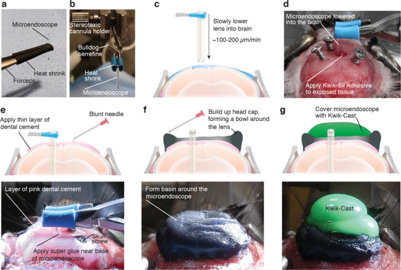
(a) Gently place the microendoscope onto the lens cloth and lightly grip it with heat shrink covered forceps. (b) Image demonstrating stereotaxic setup for stabilizing microendoscope during implantation. (c) Position microendoscope above stereotaxic coordinates for the target brain region and lower into the brain at a constant, slow rate. (d) When finished lowering the lens, place a small amount of Kwik-Sil around the lens to cover any exposed brain tissue. (e) Secure the microendoscope to the skull by carefully applying a thin layer of pink dental cement, letting it run to the lens and skull screws. Apply an additional layer of dental cement and let the cement dry for 15-mins before removing the bulldog serrefine. (f) Dislodge the lens from the holder and cover head cap with black dental cement to block outside light. Build up the remainder of the head cap by forming a protective bowl around the lens with the black dental cement. (g) Apply Kwik-Cast to protect the top of the lens. All procedures were approved by UNC IACUC.

Checking Ca²⁺ indicator expression and attachment of baseplate

CRITICAL Imaging experiments can begin when GCaMP is sufficiently expressed to allow for the detection of neural activity under the lens with a miniaturized epifluorescence microscope. The specificity of this time point will depend on brain region and cell type. In general, we have found that distinct Ca²⁺ transients can be detected from individual cells within cortical regions at an earlier time point than deep brain target structures. On average, following virus injection and lens implantation procedures Ca²⁺ transients can be distinctly visualized as soon as 2 weeks for cortical regions and 3–6 weeks for deep brain regions. Procedures for checking expression levels of GCaMP are described in procedural steps 48–65.

• 48When enough time has elapsed for sufficient expression of GCaMP (~2–6 weeks), use the miniature, epifluorescence microscope to check for Ca²⁺ signals as well as optimize the placement of a baseplate that will act as a docking station for the microscope.
• 49While holding the microscope, adjust the focusing mechanism on the microscope so that it is in the mid-range (about 1 and a half turns up from the lowest starting point) (Fig 12a). CRITICAL STEP Attaching the baseplate while the microscope is in the midrange of its focusing potential will maximize the range that microscope can be focused in either direction.
• 50Secure the focusing mechanism in the midrange position by tightening the set screw on the focusing mechanism (Fig 12a).
• 51Next, turn the set screw on the baseplate until it is flush with the edge of the baseplate and attach the baseplate to the microscope by turning the set crew on the baseplate a quarter to half a turn (Fig 12a).
• 52Attach the microscope gripper tool to a micromanipulator and secure the microscope in the gripper tool to allow the microscope to be accurately maneuvered above the implanted microendoscope. We recommend the Patchstar micromanipulator, but an articulated ball and socket mount from Thor labs may also be used as well as any other brand of quality micromanipulators.
• 53Connect the data acquisition (DAQ) box to the imaging computer with a USB 3.0 cord (Fig 12a).
• 54Connect the microscope to the DAQ box (Fig 12a).
• 55Position the stereotax under the microscope that has been secured to the microscope gripper tool. The microscope should be centered above the earbars so that the microscope is above the head of the mouse when it is secured in the stereotax.
• 56Anesthetize the mouse (we use isoflurane anesthesia)⁶⁶ and secure it in the stereotaxic apparatus (Fig 12b).
• 57Use fine forceps to remove the Kwik-Cast from the top of the microendoscope (Fig 12c). CRITICAL STEP Be careful to avoid the area underneath the Kwik-Cast where the microendoscope has been implanted.
• 58Use compressed air to clear any debris from the top of the microendoscope.
• 59Gently clean the exposed lens of the microendoscope with lens paper and 70% ethanol.
• 60Use the micromanipulator to center the objective over the microendoscope so that it is within about 2mm of the top of the lens (Fig 12d).
• 61Level the objective of the microscope relative to the microendoscope by adjusting the microscope position in the gripper tools in the medial-lateral direction and the head of the mouse in the anterior-posterior direction.
• 62Once the surface of the microscope lens objective is level with the implanted microendoscopic lens, start the imaging acquisition software and use it to adjust the settings on the microscope and to visualize cellular activity (Fig 12d).
• 63Turn on the LED of the microscope and make sure the light path of the LED is going through the center of the lens (Fig 12e).
• 64Adjust the intensity of the LED, gain, and frame rate to visualize Ca²⁺ activity. Optimal LED intensity and gain will vary by lens properties, brain region, cell type, as well as properties of the Ca²⁺ indicator, such as sensitivity, brightness, Ca²⁺ binding kinetics, and labeling efficiency^13,19. CRITICAL STEP To avoid photobleaching of fluorophores or phototoxicity, it is recommended that the intensity of the LED is set below 20% of its maximum power. However, it is important to keep in mind that light output can vary across microscopes and that the amount of light that penetrates the brain will also depend on the diameter of the lens as larger diameter lenses will allow more light to be transmitted through the lens. Thus, to determine the output of light that reaches the focal plane below the lens (~290μm below the surface of the lens), the output of the microscope LED through the GRIN lens would need to be measured for each system. It has previously been reported that the transmission of 0.05–0.20 mW of light through a GRIN lens results in virtually no photobleaching over a 20 minute imaging session²⁹, but this may vary based on the exact preparation. The effect of LED outputs above this range or recording duration on fluorescent signals would need to be tested empirically for each experimental setup.
• 65While the LED is on, use the micromanipulator to approach the surface of the lens. As you approach the lens with the micromanipulator, the top of the lens should come into focus. If the objective is level over the lens, all edges of the lens should be clear and crisp (Fig 12f). As you continue to lower the microscope close to the top of the lens, the tissue should begin to come into focus as indicated by diffuse fluorescence signals resulting from out of focus light as well as the faint outlines of vasculature (Fig 12g). When the tissue has fully come into focus, examine the quality of tissue in the field of view. The vasculature should be clearly visualized and the outlines of GCaMP expressing cells should be distinct (Fig 12h). If checking cells at an early time point (e.g., 2–3 weeks after surgery) and fluorescence signals are low, follow option A. If distinct GCaMP expressing cells can be visualized, follow option B. If fluorescence signals have the appearance of autofluorescence, follow option C. If the visual field is black, see option D. If cells can be visualized but little neural activity is seen, follow option E. If detectable Ca²⁺ signals do not appear 8–12 weeks following surgery, follow option F.

Figure 12. Checking expression of the Ca²⁺ indicator.

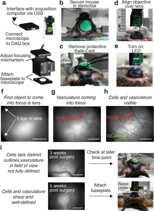
(a) Interface the miniature, integrated microscope with the acquisition computer by connecting the microscope with the baseplate attached to the DAQ box and the DAQ box to the acquisition computer. Blue arrow in inset points to set screw on microscope focusing mechanism to lock the focus in place. (b) Secure mouse in stereotaxic apparatus. (c) Remove Kwik-Cast from the top of the head cap and clean the lens with 70% ethanol and lens paper. (d) Align the objective of the microscope over the top lens of the microendoscope. The two lenses should be ~2 mm apart and parallel to each other. (e) Turn on the LED to ensure that the center of the LED is passing through the center of the microendoscope. (f) Visualize the objects under the lens utilizing the acquisition software. The first object to come into focus is the top of the lens. All the edges of the top lens should be clear and crisp if the microendoscope is level with the objective of the microscope. (g) As you move closer to the top of the lens, the vasculature and fluorescence signals will begin to come into focus. (h) The vasculature and outlines of cell bodies should be clear when in focus. (i) Example images of biological structures under the lens 3 weeks (top) and 5 weeks (bottom) post-surgery. If cell bodies and vasculature outlines are not yet clearly defined, it is ideal to wait to attach the baseplate. If the outlines of cell bodies and vasculature are clear and crisp, attach a baseplate to the head cap of the animal. Scale bar = 250 μm. All procedures were approved by UNC IACUC.

Option A) If low fluorescence levels are visualized at an early time point

1. If there are dynamic fluctuations in Ca²⁺ activity, but the fluorescence levels are low or only bulk changes in fluorescence can be visualized, it may be beneficial to wait 2–3 more weeks before attaching the baseplate. Allowing more time for the expression of GCaMP may facilitate the visualization of distinct cellular signals and therefore optimize the placement of the microscope objective relative to the implanted microendoscope.

2. In this scenario, re-apply Kwik-Cast to the lens and return the animal to its home cage.

3. Repeat steps 48–65 at a later time point. We have found 5–6 weeks following virus injection and lens implantation to be an optimal time point for the attachment of the baseplate in most of our preparations (Fig 12i).

Option B) If distinct GCaMP expressing cells can be visualized.

1. Confirm that there are dynamic changes in fluorescence activity indicative of Ca²⁺ transients by switching to the ΔF/F function on the software. If fluorescence signals are representative of Ca²⁺ transients, you should see dynamic changes in fluorescence activity. The dynamic changes in signal intensity should resemble the shapes of cells (i.e., spherical, see Fig 3) and should not correlate with tissue movement.

2. Proceed to step 66.

Option C) If autofluorescence or cell death is detected

1. If cells have died due to over expression of the Ca²⁺ indicator (Supplemental Fig 6a–c) or if fluorescence signals have the appearance of cells, but are actually autofluorescence due to tissue damage, dynamic changes in fluorescence activity will not be visualized and a baseplate should not be attached (Fig 13a–e).

2. Perfuse subject by intravascular perfusion with phosphate buffered saline (PBS) followed by paraformaldehyde^67,68. Remove brain and post-fix in PFA for 24-hrs. Following post-fixation, transfer brain to 30% sucrose in PBS for cryoprotection and keep brain in sucrose solution until it sinks to the bottom (~24–48-hrs)⁸⁰. In order to preserve the lens track in tissue, the lens can be left in the brain for 3–4 additional days while in PFA.

3. Section perfusion fixed tissue with a cryostat⁸⁰ and examine the quality of tissue near the lens as well as viral expression of GCaMP with a epifluorescence microscope⁸¹. A large amount of tissue damage near the lens track may indicate that the lens was lowered into the tissue too quickly (Fig 13a).

Figure 13. Optically detected signals not indicative of fluorescently encoded Ca²⁺ transients.

(a) Tissue damage or cell death can result in the production of fluorescence signals, referred to as autofluoresence, at the site of injury. (b) These autofluroescence signals can be detected with a 1-photon fluorescence microscope and imaged through a microendoscopic lens. Importantly, aggregates of autofluoresence signals may display similar morphological characteristics of cells (i.e., spherical spheres of fluorescence). However, unlike GCaMP6 expressing cells, signals encoding autofluorescence lack dynamic changes in signal intensity allowing these signals to be easily distinguished from those representative of neural activity. (c–d) Application of an automated cell sorting algorithm (PCA/ICA) to the data shown in b failed to extract signals representative of dynamic cellular activity. Instead, only (c) background fluorescence or (d) biological structures, such as blood vessels could be extracted from the data. e) Activity traces extracted from background fluorescence signals shown in c lack characteristic temporal dynamics of fluorescently encoded Ca²⁺ signals, further indicating that it is unlikely that the fluorescence signals detected are representative of dynamic Ca²⁺ activity. It is not recommended that a baseplate is attached if fluorescent signals have the appearance of autofluorescence. All procedures were approved by UNC IACUC.

Option D) If visual field is black

1. If the visual field under the lens is completely black, it is possible that the transmission of light is being occluded by physiological properties within the brain, such as a blood clot.

2. Perfuse the mouse (as described in option C, step ii) and visually examine the tissue below the lens.

Option E) If anesthesia suppresses neural activity

• INeural activity is oftentimes dependent on the conscious state of the animal and may be suppressed if the animal is deeply anesthetized. Gently pinch the tail of the animal or make a loud noise, such as a handclap, to try and stimulate neural activity and facilitate the visualization of Ca²⁺ dynamics. CRITICAL STEP It is possible that exposure to certain types of anesthesia may suppress the activity of specific neuronal populations, resulting in an inability to visualize dynamic changes in fluorescent activity. While we have yet to identify a population of neurons that could not be visualized within an anesthetized subject, if a neuron population is sufficiently suppressed by isoflurane to prevent its visualization, the level of anesthesia could be temporarily lowered or another type of anesthesia, such as ketamine and xylazine, could be used⁶⁶.

Option F) If there are no detectable Ca²⁺ signals after 8–12 weeks

• IIPerfuse the mouse as described in option C step ii.
• IIICheck the lens placement position relative to viral expression as described in option C, step iii.

• 66Move the position of the microscope relative to the microendoscope to select the focal plane that contains the greatest amount of healthy cells and turn off the LED. CRITICAL STEP Only proceed with this step if cells appear healthy and a sufficient level of GCaMP expression was identified in step 65. CRITICAL STEP Some adhesives may exhibit shrinkage during the drying process, resulting in a slightly lower baseplate position than intended. To minimize improper positioning of the baseplate due to shrinkage, test your adhesive prior to the baseplate attachment procedure to ensure that a significant amount of shrinkage does not occur. Alternatively, the baseplate may be secured slightly above the desired focal plane to compensate for movement that may occur during the drying process.
• 67Use black dental cement to permanently secure the baseplate to the head cap. Fill a 1 ml syringe with dental cement and attach a blunt 18G needle to the end. The dental cement should be thick and easily malleable.
• 68Begin attaching the baseplate to the head cap by building 4 pillars, one at a time, that run from each corner of the baseplate to the head cap (Fig 14a,b).
• 69Begin slowly building up dental cement from the head cap to the baseplate by filling in the four walls surrounding the baseplate (Fig 14c). Build up the anterior and two lateral walls first.
• 70When the anterior and lateral walls are complete, turn on the LED and make sure that no light escapes from these 3 walls (Fig 14d). If any light escapes, fill in cracks with dental cement.
• 71Turn off the LED and build up the posterior wall. CRITICAL STEP The posterior wall of the baseplate is shorter than the other walls so extra caution should be utilized when applying dental cement to avoid getting dental cement on the microscope.
• 72
  Before completing the dental cement application, inspect the baseplate to make sure that there is a sufficient amount of dental cement on all four walls of the baseplate so that it is securely attached to the head cap (about half way up the baseplate) (Fig 14e,f). CRITICAL STEP Be careful to avoid getting dental cement on the microscope or near the set screw located on the baseplate (Fig 14f).

  • Because the space between the baseplate and head cap is extremely narrow, it may be difficult to apply the dental cement without getting it on the microscope or near the lens. The dummy microscope can be used to practice the baseplate surgery until one feels comfortable with the procedure. To do this, attach the baseplate to the dummy microscope as described in steps 51–52 and the dummy microscope to the holder. Next, place a glass slide under the microscope and practice attaching the baseplate to the slide (Supplemental Fig 7a–c).

  CRITICAL STEP Improper baseplate attachment is the leading cause of motion artifacts and achieving optimal viscosity of the dental cement is critical to proper baseplate attachment. If the dental cement is too runny, it is possible that it will flow to the lens, and cover up the imaging surface. If the cement is too solid, it will not properly adhere to the baseplate, increasing the probability of movement noise.

• 73Once the dental cement has completely dried (Fig 14g), dislodge the microscope from the gripper tool and move the micromanipulator arm away from the microscope (Fig 14h). The microscope should remain stable on the mouse’s head during this process.
• 74Use the hex key to loosen the set-screw on the baseplate (Fig 14i). Gently pull the microscope away from the baseplate while holding the mouse’s head down with the other hand (Fig 14j).
• 75Carefully place the microscope back in its case.
• 76Attach the dust cap to the baseplate. Similar to above, turn the set-screw on the baseplate so that it is flush with the baseplate. Attach the dust cap to the baseplate and tighten the set screw 0.25 to 0.5 turns until the dust cap is securely attached to the baseplate (Fig 14k). Allow the mouse to recover for 2 to 3 days before beginning habituation procedures or behavioral testing.

Figure 14. Attachment of baseplate.

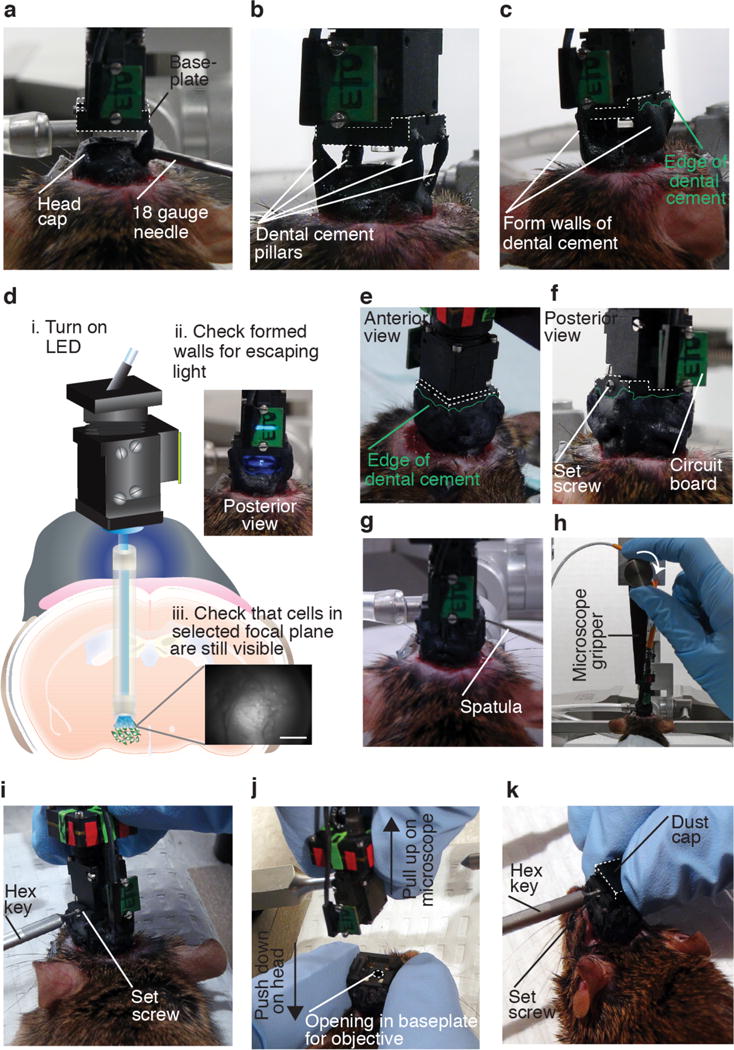
(a) Begin attaching the baseplate (outlined with white dotted line) to the head cap by forming pillars of black dental cement from the baseplate to the head cap. (b) Form 4 pillars in total, 1 at each corner of the baseplate. (c) Build up all remaining walls of the head cap (edge of dental cement outlined in green). (d) Before building up the final posterior wall, turn on the LED and make sure that no light escapes from the completed walls. Fill in any cracks where light escapes and complete the baseplate attachment procedure by filling in the posterior wall. Once all walls have been filled, cells and vasculature that were visible when the focal plane was selected should be visible when the LED is turned on. Scale bar = 250 μm. (e) Example image of anterior and lateral wall of head cap with the dental cement going about half way up the baseplate. (f) Example image of posterior wall and lateral wall of the baseplate where the set screw is located. The posterior wall of the baseplate is shorter than the other 3 walls so caution should be taken when applying dental cement to this region. Caution should also be taken when applying dental cement near the set screw of the baseplate or when in close proximity to the microscope circuit board. (g) Before removing the microscope, test to make sure the dental cement has completely dried (~15 min) by scratching the exterior with a spatula. Process should make a scratching sound once the cement has hardened. (h) Once the dental cement has dried, dislodge the microscope from the microscope gripper. (i) Use the hex key to loosen the baseplate set screw. (j) Remove the microscope by gently pulling up on the microscope while applying slight downward pressure to the mouse’s head. (k) Secure dust cap on baseplate to protect the top of the lens by locking dust cap in place with set screw. All procedures were approved by UNC IACUC.

Preparation for in vivo monitoring of neural activity in freely behaving mice

• 77Although the microscope is extremely lightweight (~2g), some mice take time to adjust to the attachment process and initially have difficulty maneuvering through their environment with the microscope attached. If it seems necessary, habituate the mouse to these procedures, by using a dummy scope secured to a tether with similar physical and mechanical properties as the microscope cable (Supplemental Fig 8a) and place the mouse in a behavioral testing setup that will be used during the experimental procedure^42,75 (Supplemental Fig 8b). When the mouse appears to be moving normally through its environment (i.e., unrestricted active forward locomotion and turning behavior) proceed to the next steps to begin in vivo imaging experiments.
• 78Make sure that the computer used for imaging has enough space to store the data. For example, 30-mins of data acquired at 20 Hz requires ~110 GB of space. CRITICAL STEP Check this before beginning a behavioral recording session to avoid data loss.
• 79Connect the microscope imaging system to the acquisition computer as described in procedural steps 53 and 54.
• 80To attach the microscope, anesthetize the mouse with isofluorane.
• 81Place the mouse on a heating pad with its nose positioned in front a re-breathable nose cone apparatus to maintain gas anesthesia (Fig 15a).
• 82Remove the lens cover from the microscope and use the hex key to remove the dust cap from the baseplate (Fig 15a).
• 83Turn the set screw on the baseplate so that it is flush with the inner wall of the baseplate and attach the microscope to the baseplate (Fig 15b) by turning the set screw on the baseplate 0.25 to 0.50 turns. CRITICAL STEP It is essential that the set screw for the focusing mechanism or baseplate are never over tightened. When securing the microscope or the focusing mechanism in place, both screws should never be turned more than a 0.25 to 0.5 of a turn. Turning of the screw should be stopped as soon as any resistance is felt. Over tightening the set screw may result in the microscope to become dislodged during the recording or possibly damaged.
• 84Start the data acquisition software. Adjust the frame rate, LED intensity, and gain to visualize cellular activity. As described in step 64, it is best to keep the intensity of the LED between 10 and 20% of its maximum power to avoid photobleaching or cell death as a result of phototoxicity. If the signal still needs to be amplified after this point, compensate for a low signal by either increasing the exposure time (i.e., the length of time in which light is collected for a given frame) or adjusting the gain.
• 85Adjust the focusing mechanism on the microscope to increase or reduce the distance of the sensor from the focal plane until cells and vasculature are clearly in focus (Fig 15c).

  TROUBLE SHOOTING

• 86
  Once the focal plane has been selected, lock the focusing mechanism in place with the set screw (Fig. 15d). Allow the mouse to recover with the microscope attached to its head in a secure cage for at least 20–45 minutes before beginning behavioral recording session (Fig. 15g)^29,42. CRITICAL STEP The use of anesthesia, even over brief periods, may result in long-term suppression of neural activity. Confirm recovery from anesthesia by observing normal animal movement and a return to baseline levels of neural activity. It may also be beneficial to conduct recordings of the target cell population as the mouse recovers from anesthesia to determine the amount of time it takes for anesthesia induced changes in neural activity to wear off. Finally, it is important that all mice are given the same amount of time to recover from anesthesia before beginning a recording session to control for any remaining anesthesia induced changes in neural activity.

  • If the use of anesthesia poses a significant confound to your experimental design, it is possible to tether the mouse by having one person manually restrain the mouse while another person removes the dust cap and secures the microscope. However, the use of manual restraint to attach the microscope is not without confound as it will likely induce stress in the test subject. For this reason, it is important to habituate the test subject to the attachment procedure and allow the mouse sufficient time to recover. It is also important that all test subjects undergo similar microscope attachment procedures.
• 87When sufficient time has elapsed to allow the mouse to fully recover from anesthesia, place the mouse in the behavioral recording chamber.
• 88If the microscope that you are using does not allow for the use of a commutator, secure the microscope cable at a point high above the floor of the chamber where the recording session is to be conducted (~120 cm). Securing the microscope cable at a distance high above the base of the recoding chamber will reduce the amount of twisting in the cable that often occurs near the top of the microscope. Additionally, attaching the cable to an object with the ability to stretch, such as a rubber coil, or a small object with a turning mechanism, such as a ball bearing swivel, will further reduce strain on the cable and facilitate animal movement.
• 89Once the cable is secure, ensure that there is sufficient slack in the cable to allow the animal to freely roam about the testing chamber. Given that both the microscope and attached cable are light enough to be carried on the head of the mouse without the necessity of external support, an optimal configuration of the tether provides enough slack so that the mouse can freely move about its environment without the tether hanging below the head of the mouse. If the cable is too tight, it will result in excessive strain on the cable, possibly resulting in damage to the thin copper wires located within the cable and a subsequent loss of data. Alternatively, if the cable is too loose, the animal may be able to access it and bite through the thin wires.
• 90Open the acquisition software and select the frame rate that is optimal for your neuron population and indicator (Fig 15f). Typically, it is ideal to select the variant of GCaMP (i.e., fast, medium, or slow) based on the physiological properties of the specific neuronal population and the frame rate based on the kinetic properties based of the indicator. CRITICAL STEP It is important to keep in mind that a higher frame rate will reduce the intensity of the detected signal (indicated by a lower mean pixel intensity) as a result of a reduction in exposure time. Thus, to reduce the possibility of photobleaching, it is best to not record at a frame rate that is higher than necessary to accurately detect the neuronal signal. Additionally, higher frame rates increase the amount of acquired data, potentially leading to unnecessarily high data storage cost as well as an increase in data analysis time.

  TROUBLE SHOOTING

• 91Next, turn on the LED and adjust the LED intensity and gain to maximize the fluorescence signal. If provided by your acquisition software, use the mean intensity pixel value feature to facilitate the selection of LED intensity and gain. To achieve pixel values within the recommended intensity range of 1500–3000, first adjust the LED intensity to up to 20% of its maximum intensity. Adjusting the LED intensity produces the least amount of noise when enhancing signal detection.

  TROUBLE SHOOTING

• 92If signal intensity is not sufficiently high, adjust the gain to digitally enhance signal brightness. Keep in mind that using the gain to adjust signal intensity will also increase noise so it is recommended that gain is kept at 1 when possible. A threshold indicator feature may be used to ensure that the LED and gain are not excessively high as to result in signal clipping or phtobleaching/photoxicity. CRITICAL STEP We have found that a mean intensity pixel value ~3000 works well for most recording regions and neuron populations. It is recommended that the mean pixel intensity does not fall below 1500. A pixel value below this range may make it difficult to extract significant cellular signals from the acquired images. Conversely, a mean pixel value above 4000 may over expose the tissue, resulting in photobleaching or phototoxicity. CRITICAL STEP Long-term recording sessions (i.e., greater than 20-mins) have an increased risk for photbleaching, photoxicity, and potential tissue damage due to heating of the tissue by the LED. It is recommended that frame rate, LED, and Gain settings are adjusted as described in this protocol to minimize photobleaching. Although tissue heating has not been directly tested (or reported) in response to exposure to light produced by LEDs located within miniaturized microscope systems, prior studies using micro inorganic LEDs directly implanted in brain tissue have reported LED induced increases in tissue temperature as a function of stimulation frequency over time⁸². However, we have measured the output of light directly from the objective lens of the microscope and found that light output produced by the LEDs located in miniature microscopic systems falls well below the range of light intensities associated with heating of neural tissue^82,83. Thus, we predict that tissue heating due to the LED should be negligible.
• 93For experiments that require multiple recording sessions, a snapshot of the imaging site can be taken on the first imaging session to facilitate repeatedly imaging the same field of view. On future imaging sessions, the snapshot can then be uploaded into the imaging software and overlaid on top of the live image to ensure that the biological structures underneath the lens appropriately align. For example, if using nVista recording software, this can be accomplished by selecting overlay options under visualization tools and uploading a TIFF file that is representative of the focal plane from the previous recording session. Next, adjust the opacity of the TIFF image so that the live image can be visualized underneath the TIFF image. The focal plan can then be adjusted with the microscope focusing mechanism until the location and size of anatomical structures is consistent between recording sessions. Additionally, the number of turns that the focusing mechanism was adjusted from its lowest point can be counted by placing evenly spaced tick marks around the top of the focusing mechanism. An example of such tick marks can be seen in figure 15 c and d. By combining both suggested methods, we have successfully imaged the same neuronal population across multiple imaging sessions in 1 mouse (Supplemental Fig 9a,b). We further maximized repeated cell identification by applying an image registration algorithm to the extracted spatial maps (Supplemental Fig 9c–e).
• 94Allow the mouse sufficient time to recover from anesthesia and habituate to the recording session.

  TROUBLE SHOOTING

• 95Immediately before beginning an imaging session check the settings of the gain and the LED to ensure that the settings are optimal. Although the intensity of the LED and gain may have been adjusted to visualize cells while adjusting the focus of the microscope, it is common for anesthesia to suppress neural activity and thus the settings used to initially visualize the cells may be higher than those needed for signal detection in an awake freely behaving animal. If needed, adjust settings.
• 96For experimental procedures that do not require the acquisition software to be triggered by an external program, follow option A. For experiments that require the acquisition of imaging data to be synchronized with a behavioral acquisition system, see option B. CRITICAL STEP For both option A and B, it is important to consistently monitor the animal and cable throughout the duration of the imaging session. Additionally, while imaging, nonessential applications on the computer should be closed to reduce the risk of the data acquisition crashing during a recording session.

Figure 15. Visualization of Ca²⁺ transients in freely behaving mice.

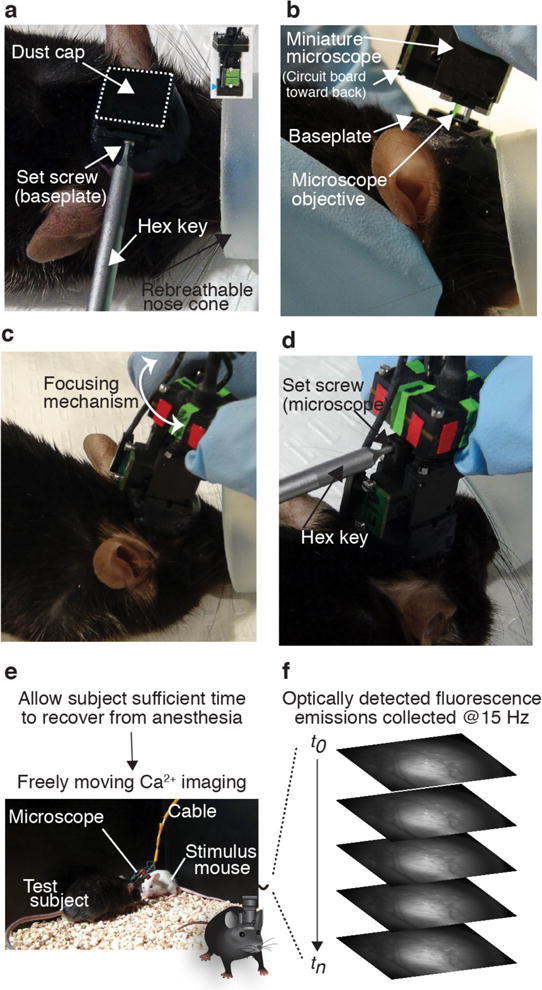
(a) Anesthetize mouse and remove dust cap (b) Mount microscope to baseplate. (c) Adjust focusing mechanism to bring cell bodies and vasculature into focus. (d) Tighten the set screw on the focusing mechanism once the focal plane has been selected. (e) Following anesthesia recovery period, conduct Ca²⁺ imaging during naturalistic, unrestrained behavior. (f) 2-dimensional x–y image stacks of raw Ca²⁺ imaging data acquired during an in vivo imaging session.

Option A) For non-synchronized recordings

1. Adjust the recording schedule in the acquisition software to automatically set the duration of the recording session.

2. Select ‘Record’ in the imaging acquisition software to begin an imaging session.

Option B) To synchronize imaging data with behavioral monitoring software

1. A recording session can also be triggered by coupling the acquisition software with commonly used behavioral recording software, such as VideoTrack (ViewPoint Behavior Technology)⁴², Ethovision (Noldus)²⁶, or Med Associates behavioral equipment²⁶. Triggering the microscope in this manner will allow the imaging data to be synchronized with behavioral data.

2. If utilizing the nVista imaging system, the DAQ box contains a BNC port labeled “trigInput” that allows it to receive signals to trigger the start and stop of an imaging session from another software.

3. To trigger an imaging session via an external program, connect the BNC output cable from the behavioral recording system to the trigInput port on the DAQ box.

4. Press start on your designated behavioral recording software to trigger the imaging acquisition software. CRITCAL STEP In our experience, behavioral recording systems that send low output voltage signals work best when integrating the DAQ box with behavioral acquisition software. If your system sends a high output signal, an Arduino microcontroller or a simple circuit utilizing a transistor can convert this signal to a low output (and maintain the base state at high). CRITICAL STEP We have also found that it is best to run the imaging acquisition software and the behavioral acquisition software on separate computer systems.

• 97Once the imaging session is complete, anesthetize the mouse with isoflurane and disconnect the microscope from the baseplate.
• 98Coil the cable of the microscope gently to avoid kinking or twisting the wire. Kinks or twists in the wire can result in dropped frames and therefore a loss of data.
• 99Attach the dust cap to the baseplate as described in procedural step 76 and allow the animal to wake up from anesthesia in a secure cage.

Data pre-processing steps and conversion to Δ F/F format

CRITICAL STEP The ideal method for signal extraction and data analysis will depend on multiple variables related to the quality of the data, such as signal to noise ratio, general physiological properties of the neurons, such as firing rate, as well as the anatomical organization of the neurons within the imaging region, such as cell density. Nonetheless, for most data sets, some general pre-processing steps can be applied, as described in steps 99 and 100 (Supplemental Fig 10).

• 100
  To increase data processing speed, reduce the size of the data files by binning the data in the spatial (i.e., average in space) and/or temporal (i.e., average in time) domain^26,29,42 with the use of custom software written in MATLAB²⁹, Mosaic analysis software²⁶, or ImageJ.

  • Spatially binning imaging data can facilitate the analysis process in two ways. First, spatially binning the data can speed up the analysis process by reducing the file size of the movie. Second, spatially binning the data can smooth the edges between contrasting structures, which acts to improve the accuracy of the motion correction algorithm, especially in cases where a larger number of frame shifts occurs. We have used Mosaic analysis software to spatially bin Ca²⁺ imaging data collected under imaging conditions that vary by imaging depth, lens diameter, brain region, and neuron population and have that a spatial bin of 4 works well for most data sets^26,29. CRITICAL STEP Spatial binning of the data will reduce the number of pixels in each frame. Thus, when spatially binning the data, the spatially binned data set should be inspected to ensure that distinct biological structures can still be clearly visualized (Supplemental Fig 10a).
  • If the sampling rate of the movie is at a higher temporal resolution than is necessary for the analysis of cellular activity, the data can be temporally binned for faster execution of future data processing steps (Supplemental Fig 10b). For most neuron populations, we acquire data at 15 Hz and have found that a temporal bin of 3 (down sample to 5 Hz) sufficiently reduces the size of the data without obscuring transient Ca²⁺ signals²⁶. Other groups have reported similar down sampling procedures in brain regions such as the hippocampus²⁹. CRITICAL STEP Temporal binning of the data will reduce the total number of frames and therefore the number of time points in which the signal was sampled. When temporally binning the data, the dynamic properties of the neuronal population as well as the Ca²⁺ indicator should be considered so that the frame rate is sufficient to adequately detect Ca²⁺ transients. It is not recommended that the data be temporally binned to a rate that is slower than the binding kinetics of Ca²⁺ indicator (rise time + 0.5 the decay time).

  TROUBLE SHOOTING

• 101It is common for drift or frame shifts to occur within a given imaging session, interfering with the detection of biological signals across time. To increase the accuracy of signal detection, reduce motion artifacts through the application of a motion correction algorithm to either the raw or binned data set^64,84. ImageJ and Mosaic analysis software contain plugins or built in algorithms, respectively, for the motion correction of Ca²⁺ imaging data²⁶. There are multiple types of motion correction algorithms that can be used with the above software, such as intensity or feature based algorithms that are suitable for Ca²⁺ imaging data. For most data sets, we have successfully reduced motion artifacts by the application of a rigid body translation algorithm (similar to the TurboReg plugin for ImagJ) available in the Mosaic analysis software package (Supplemental Fig. 10c).
• 102After completing the preprocessing steps (dimension reduction and motion correction), convert video files to a ΔF/F format^26,29,56, which represents the percent change in fluorescence over baseline. This conversion can be accomplished with custom code written in MATLAB²⁹, Image J⁷⁵, or Mosaic analysis software²⁶ (See supplemental videos for an example of a raw Ca²⁺ imaging data set (Supplemental video 2) that was processed as described in procedural step 100–102 (Supplemental video 3–7). Supplemental Fig 11 provides information that was used to apply the motion correction algorithm. See Anticipated Results for more analysis information).

Anatomical verification of microendoscope placement

• 103Following the completion of an experiment (i.e., all planned imaging sessions within a subject), confirm anatomical placement of the lens above the neuronal population of interest⁴².

  TROUBLESHOOTING

  See Table 3 for suggested solutions for problems that may occur in the procedure.

Table 3.

TROUBLESHOOTING TABLE.

Steps	Problem	Possible Reason	Solution
11	Low level or absence of viral expression	Sparse expression of Ca2+ indicator due to low virus dilution, or inadequate injection volume	Decrease the amount of saline per volume of virus or increase the injection volume per site. Multiple injection locations spaced a few hundred microns away from each other may also help increase viral spread
		Viral serotype cannot or insufficiently transfects cell type of interest	Choose a viral serotype that has a high affinity for cell population of interest. We have found the AAVdj serotype to work well in many cell populations.
		Insufficient viral expression time	Increase time allowed for viral expression.
21 & 22		Dura or bone debris physically obstructing diffusion of virus into the brain	Make sure that dura is completely removed before performing virus infusion. Dura has a yellow tinge compared to brain tissue and the tissue should appear white when all dura has been removed. Remove any skull fragments before beginning viral injection.
1 & 2	Over-expression of viral indicator (i.e., cells do not have a honey comb appearance)	Concentration or volume of injected virus is too high	Dilute virus in sterile saline or reduce injection volume.
12	Virus expression or lens location not in target area	Stereotaxic coordinates inaccurate	Re-evaluate stereotaxic coordinates of target structure
		Animal’s skull was not level during surgery	Level the anterior-posterior and medial-lateral axes of the skull until the distance between bregma and lambda in the dorsal-ventral direction is less than 0.05 mm
24 & 25	Excessive tissue damage at site of lens implantation	Brain tissue improperly aspirated (only for deeper lens implantations)	Before lowering microendoscope into neural tissue, aspirate 1 to 3 mm of tissue above target neuron population.
34		Microendoscope lowered into tissue too quickly	Incrementally lower the lens into the tissue at a rate of 100–200μm/min. Allow the tissue to settle between each 100–200μm lowered. Retract the lens +/−500 um for every 1 mm lowered.
13	Excessive movement noise in acquired data	Connective tissue and/or muscle was not sufficiently retracted and removed from the skull	Amend surgery protocol for a more thorough clearing of connective tissue and muscle tissue before implantation of the microendoscope
28 & 36		Headcap insufficiently secured to the skull	Apply dental acrylic or metabond to skull before application of dental cement. Placement of the skull screws should be at a medium distance away from the craniotomy. We recommend placing the skull screws about 1.5 cm away from the lens implantation site.
90–92	Low level or absence of detected fluorescence emission	Inadequate exposure time, gain, or LED intensity	Increase exposure time on Ca2+ acquisition software. 66.67 ms exposure time (15 Hz) is ideal. Increasing the gain may also be a solution
6		Inappropriate lens position	Perfuse the mouse and check the position of the lens, relative to the target neuron population. The lens should be placed about 300 μm above GCaMP expressing cells
1–3		Inadequate viral expression of Ca2+ indicator	Perfuse the mouse and check the viral expression levels. If few cells are expressing the indicator, decrease the virus dilution. *Note it is recommended to wait at least 6 weeks before perfusing an animal as it can take up to 6 weeks for clear images to be achieved in deep brain structures.
24 & 25	Fluorescence emissions do not exhibit dynamic changes in fluorescence signal	Fluorescence signal may be representative of autofluorescence and not the expression of a Ca2+ indicator	Aspirate tissue above microendoscope implantation to remove pressure underneath microendoscope.
34			Lower microendoscope at a rate of about 100–200 μm/minute.
26			Inject virus at a distance that is not immediately underneath the lens, about 250 μm away
91–94	Inability to extract ICs from Ca2+ data	Emitted Fluorescent signal is too low for detection.	Increase the LED intensity to up to 20% of its maximum power. Compensate with the gain to further increase the detection of the fluorescence signal. If the signal cannot be increased to achieve high enough detection levels by adjusting the LED or gain, try allowing more time for viral expression or decrease the dilution of the virus in future mice.
85		Cells are not in the plane of focus, resulting in diffuse spatial filters	Adjust the focusing mechanism on the microscope so that the outline of the cells and vasculature appears crisp
100	Data extraction process extremely slow	Size of data file too large	Reduce the data file size through temporal and/or spatial binning
		Not enough memory installed on computer	Install more memory cards to the analysis computer. It is recommended that the computer have at least 16 GB of RAM. You may also consider using a cluster computer system, such as Spark, or research cluster computing resources at your local institution.

TIMING

• Steps 1–6: Virus dilution study and selection of lens, 3 weeks to 2 months

• Steps 7–47: Virus injection and lens implantation, 2–3 h

• Steps 48–76: Attachment of baseplate, ~ 2 h

• Steps 77–99: In vivo imaging in freely behaving mice, 1–2 h per session depending on behavioral paradigm

• Step 100–101: Pre-processing steps for data analysis ~2 h

• Step 102: anatomical verification of microendoscope placement ~2 h

ANTICIPATED RESULTS

Successful completion of this protocol permits the visualization of active neural ensembles located within both superficial and deep brain regions of freely behaving mice²⁶. Figure 16 shows representative examples of in vivo Ca²⁺ imaging data collected from cortical (a–f), subcortical (g–i), and deep brain areas (m–r) of mice as they actively engage with their environment. These data were collected using the procedural steps outlined in this protocol by various members of our laboratory, demonstrating that this protocol can be easily adapted by multiple users and applied to a wide variety of brain structures. Further examples of typical results obtained by our laboratory can be found in reference 26. To obtain similar results, in the following section, we briefly describe currently available methods to extract Ca²⁺ transients from spatially defined cells. We also provide references (when available) to direct readers to studies that have utilized these data extraction methods in conjunction with imaging procedures similar to those described in this protocol (I.e., a miniaturized-epiflourescence microscope used in conjunction with a microendoscopic lens).

Figure 16. Example of in vivo Ca²⁺ imaging data collected from superficial, subcortical, and deep brain regions.

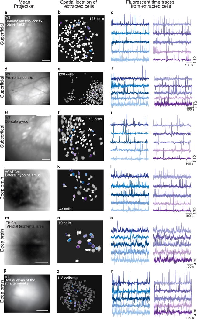
The protocol described here can be adapted for successful in vivo recordings of Ca²⁺ transients within superficial (a–f), subcortical (g–i), and (j–r) deep brain regions of freely behaving mice. All examples are from one 10-min acute recording session (1 mouse/brain region, data acquired @15 Hz, temporally down sampled to 5 Hz, spatial bin of 4). A 1mm diameter lens was used to image Ca²⁺ signals in superficial and subcortical areas, while a 0.5 mm diameter lens was in deep brain regions. The left column shows digital images generated by creating a mean intensity projection of fluorescence activity across the entire recording session, the middle column shows the spatial location of optically detected GCaMP expressing cells, and the right column shows activity traces (variation from the mean fluorescence signal over time) of cells outlined in the corresponding spatial map. Spatial maps and activity traces were extracted with PCA/ICA analysis (Mosaic analysis software, Inscopix). (a–c) Somatosensory cortex neurons were targeted by injecting AAVdj-CamkII-GCaMP6f (Titer: 5.6 × 10¹², 1:8 dilution, UNC vector core) into the barrel field region of an adult male wild-type (WT) mouse. (d–f) Prefrontal cortex neurons were targeted by injecting AAV-DJ-CamkIIa-GCaMP6s into the prefrontal cortex of an adult male WT mouse (Titer: 5.3 × 10¹², 1:6 dilution, UNC vector core). (g-i) AAV-DJ-CamkIIa-GCaMP6m was injected into the dentate gyrus of WT male mice (Titer: 7.0 × 10¹², 1:1 dilution, Stanford). (j–l) GCaMP6m was targeted to GABAergic neurons within the lateral hypothalamus by injecting AAVdj-EF1a-DIO-DIO-GCaMP6m (Titer 9.7 × 10¹², 1:2 dilution, Stanford) into adult male VGAT-Cre mice. (m–o) Dopamine neurons within the ventral tegmental area (VTA) of an adult male mouse were targeted by injecting AAVdj-EF1a-DIO-DIO-GCaMP6m (Titer 9.7 × 10¹², 1:2 dilution, Stanford) into a TH-Cre mouse. (p–r) Bed nucleus of the stria terminalis (BNST) neurons were targeted by injecting AAV-DJ-CamkIIa-GCaMP6s (Titer: 5.3 × 10¹², 1:6 dilution, UNC vector core) into wild-type mouse. Notice that deep brain regions differ from cortical regions in image clarity. Injection volumes for all regions were 300 μl. Scale bar = 125 μm. All procedures were approved by UNC IACUC.

Extraction of individual cellular Ca²⁺ signals from high dimension data sets

An advantage of Ca²⁺ imaging is the potential to simultaneously monitor the activity of large neural networks. However, this sampling method produces data sets of high dimensionality (n_pixels × n_frames) and extracting meaningful biological signals from imaging data requires the deconvolution of the data into independent signal sources^85,86. This task can be difficult for multiple reasons. First, 1-photon microscopy lacks optical sectioning abilities^14,20,23, resulting in fluorescent signals from cells located within and out of the focal plane to both be detected by the photosensor located within the head-mounted microscope⁸⁵ (Supplemental Fig 12a). This aspect of 1-photon microscopy increases the potential for signal crosstalk and methods for disentangling the neural dynamics of optically detected cells within the focal plane from those out of the focal plane are therefore necessary. Cellular crosstalk can also occur if cells within the focal plane overlap in anatomical space as these cells will also have overlapping pixel sets⁸⁵. This specific potential for signal crosstalk is particularly high when imaging densely populated networks (i.e., greater than 50 cells in the field of view). Finally, the large size of Ca²⁺ imaging data sets (many pixels collected over multiple frames) can make the analysis process extremely labor intensive (Supplemental Fig 12b). Thus, to facilitate the extraction of transient Ca²⁺ activity from spatially defined biological structures, multiple data analysis methods and computational techniques have been developed^85–88 (Supplemental Fig 12c). Below, we briefly describe some of the currently available methods for decomposing high dimensionality imaging data into individual cellular signals.

A conventional method for segmenting Ca²⁺ imaging data into individual cellular signals is region of interest (ROI) analysis. With ROI analysis, spatial clusters of pixels are assigned to individual cells, by visually inspecting the data and manually circling pixels that have characteristic morphological properties of a GCaMP expressing cell. Temporal information related to dynamic Ca²⁺ activity is then extracted by converting pixel intensity values within an identified ROI into a ΔF/F trace³². This analysis method can be conducted with Mosaic analysis software, a free plugin available for ImageJ⁷⁵, or custom software written in MATLAB or Python⁵⁶. Importantly, ROI analysis has been used to successfully extract transient Ca²⁺ activity from individual cells that were visualized with imaging procedures similar to those described in this protocol. Specifically it was used to extract the activity of individual neurons located within the entorhinal cortex of male mice (~40/mouse)⁷⁵ as well as the activity pattern of neurons located within the premotor nucleus of male zebra finches (reported 167 neurons across 9 birds; estimated to be ~18/bird)⁵⁶.

Although ROI analysis has been successfully utilized to isolate individual cellular Ca²⁺ transients from data sets that contain a relatively low number of identified cells (<40/subject), it may not be well suited or feasible to extract individual cellular signals from Ca²⁺ imaging data sets where the activity of a large number of independent cellular signals can be detected. Specifically, for Ca²⁺ imaging data sets that contain a high density of GCaMP expressing cells^26,29, ROI analysis may not permit cells that have full or partially overlapping boundaries with each other to be manually disentangled from each other. In addition, due to a lack of optical sectioning, it is possible for fluctuations in fluorescence intensity within an ROI to be associated with a cell that was manually identified by the experimenter as well as fluctuations in neural activity that are occurring above and/or below this cell. To account for these limitation in ROI analysis, efforts have been made to reduce signal crosstalk with ROI analysis through semi-automated morphological filtering of cellular signals⁸⁷, the use of temporal-cross correlation algorithm to identify highly correlated pixels within a ROI⁸⁸, as well as computational methods to correct for signal contamination by out of focus fluorescence⁸⁹. Finally, because the user must manually define the spatial location of each cell, this type of analysis can be extremely labor intensive⁸⁵. Thus, ROI analysis is best suited for datasets that contain relatively sparse populations of neurons that do not overlap in space⁵⁶.

For large data sets that contain a high density of neurons, automated cell sorting algorithms may be better suited to extract spatial and temporal properties of individual cellular Ca²⁺ signals^85,90. For example, two software packages, Thunder⁵³ (See supplemental information for code) and Mosaic (Inscopix) provide automated cell-sorting algorithm to extract data from digitally collected images. In brief, this algorithm first runs principal component analysis (PCA) to reduce the dimensionality of the data by removing signals that mostly encode noise. Dimension reduction is then followed by independent component analysis (ICA) to identify the spatial and temporal properties of visualized cells by segmenting the data into statistically independent spatial and temporal signals⁸⁵. The extracted signals, or independent components, are than manually sorted to confirm that the extracted data is representative of cellular Ca²⁺ transients from spatially defined GCaMP expressing cells^26,29. Because PCA/ICA analysis relies on statistical independence of signals, it out performs ROI analysis in the reduction of signal crosstalk and can be used to relatively quickly extract independent cellular signals from relatively large data sets⁸⁵. For example, for optical imaging data collected with the methods described in this protocol, PCA/ICA analysis has been used to successfully extract signals from up to a 1,000 neurons in the hippocampus^29,42, 100s of neurons in the lateral hypothalamus²⁶, as well as 100s of neurons in the medial entorhinal cortex⁶⁵. In addition to these densely populated networks, PCA/ICA analysis has also been used to successfully extract individual cellular signals from relatively sparse neuronal populations, such as AGRP neurons located within the arcuate nucleus of the hypothalamus (61–99 neurons/4 mice)²⁷.

Although PCA/ICA is superior to ROI analysis in some areas of data extraction (I.e., analysis speed and crosstalk reduction), it is important to note that this computational method also has limitations that can reduce the accuracy of data interpretation. First, the number of independent components to be extracted from the data set must be specified by the experimenter prior to the analysis. This is usually done by estimating the number of active cells following visual inspection of the digitally acquired dataset and setting the number of independent components to be larger than this number^26,29,65. As can be expected, the quality of cell extraction is partially dependent on this estimate. For instance, if the number of independent components is set to be much larger than the number of cells in the data, PCA/ICA may separate individual cells into multiple components. Additionally, the PCA/ICA algorithm is stochastic. Hence, there is a high probability that the extracted components will not exactly be the same across multiple runs of the algorithm, even on the same data set. Thus, when applying this algorithm to datasets collected across multiple imaging sessions, a conservative approach may be to first run PCA/ICA to extract the cellular signals and then, based on the cells spatial filter (i.e., x,y pixel coordinates associated with that cell), only select cells that have been consistently identified across imaging sessions²⁷. Finally, because this analysis method relies on the identification of statistically independent signals, it may not be well suited for the analysis of neural ensembles with low activity levels that do not substantially differ from baseline⁸⁵. In this case, ROI analysis may be better suited to extract Ca²⁺ activity traces from independent cellular signals.

Other published automated cell sorting algorithms include non-negative matrix factorization⁸⁶ or a matrix factorization that explicitly models calcium fluorescence dynamics⁹⁰. As yet, no paper has systematically benchmarked these methods against each other. Hence, it is currently unclear which method is best suited for Ca²⁺ indicator data from epifluorescence microendoscopy. In addition, to our knowledge, this analysis method has also not been used to analyze Ca²⁺ imaging data obtained by the methods described in this protocol.

Correlation of neural activity with experimental manipulations, environmental context, or behavioral events

Once the spatial and temporal data has been extracted, the activity of cells can be correlated with contextual changes in environment^65,75, environmental exploration^26,42,65,75, time-locked stimulus presentations or behavioral events²⁶, learning or experience mediated plasticity within networks^29,56, as well as pharmacological induced alterations of network activity⁴² (Fig. 17a). Perhaps the most significant advantage provided by this technique, is the ability to further analyze the data in relation to the spatial location of cells, providing activity maps or information related to functional connectivity within identified microcircuits (Fig. 17b, See supplemental information for further analysis instructions). Importantly, the ability to image cell type specific activity during naturalistic animal behavior allows this imaging protocol to be applied to a wide array of experimental manipulations to answer questions that were unable to be explored with previous methods for monitoring of neural activity.

Figure 17. Correlation of optically detected neural activity with time-locked events.

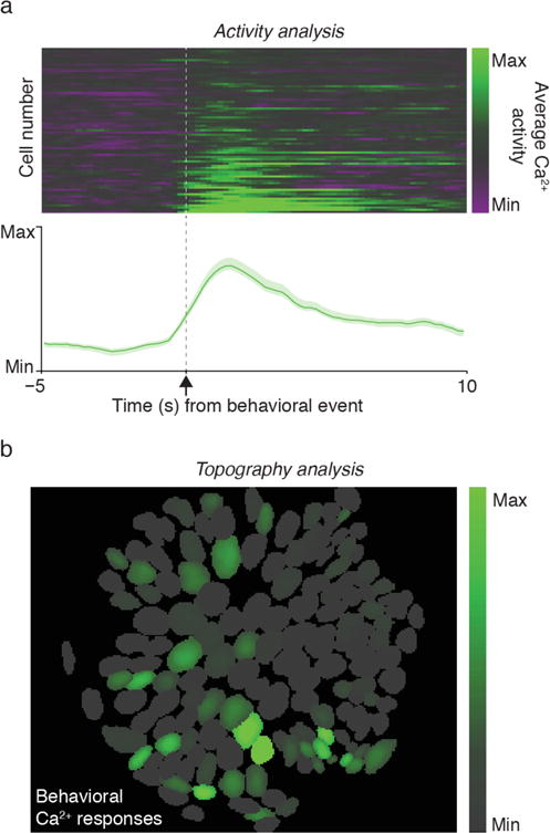
The methods outlined in this procedure permit the activity of neurons to be monitored with cellular level resolution as mice perform naturalistic behaviors. (a) When this method is further combined with simultaneous time-locked recordings of environmental, behavioral, or pharmacological events the activity of optically detected neurons can be sorted by their response profile to specific stimuli or behavioral events. In this example, GABAergic neurons within the lateral hypothalamus of adult male mice (n = 6) were monitored during consummatory licks for a sucrose reward. 75 cells out of 743 total identified cells showed excitatory responses to reward consumption. The average response of each cell was averaged across trials and aligned to the lick response (5 seconds before and 10 seconds after). (b) Cell activity map from a representative animal shows response of each neuron to consumption of sucrose reward (average difference in fluorescence intensity 1.5 s before and after the event). All procedures were approved by UNC IACUC. See supplemental methods for instructions on how to conduct similar analysis. Panels adapted from Jennings et al., 2015.

References

- 1.Chorev E, Epsztein J, Houweling AR, Lee AK, Brecht M. Electrophysiological recordings from behaving animals–going beyond spikes. Curr Opin Neurobiol. 2009;19:513–519. doi: 10.1016/j.conb.2009.08.005. [DOI] [PubMed] [Google Scholar]
- 2.Hubel DH. Single unit activity in lateral geniculate body and optic tract of unrestrained cats. J Physiol. 1960;150:91–104. doi: 10.1113/jphysiol.1960.sp006375. [DOI] [PMC free article] [PubMed] [Google Scholar]
- 3.Clark JJ, et al. Chronic microsensors for longitudinal, subsecond dopamine detection in behaving animals. Nat Methods. 2010;7:126–129. doi: 10.1038/nmeth.1412. [DOI] [PMC free article] [PubMed] [Google Scholar]
- 4.Robinson DL, Venton BJ, Heien MLAV, Wightman RM. Detecting subsecond dopamine release with fast-scan cyclic voltammetry in vivo. Clin Chem. 2003;49:1763–1773. doi: 10.1373/49.10.1763. [DOI] [PubMed] [Google Scholar]
- 5.Miyawaki A, et al. Fluorescent indicators for Ca2+ based on green fluorescent proteins and calmodulin. Nature. 1997;388:882–887. doi: 10.1038/42264. [DOI] [PubMed] [Google Scholar]
- 6.Akerboom J, et al. Optimization of a GCaMP calcium indicator for neural activity imaging. J Neurosci Off J Soc Neurosci. 2012;32:13819–13840. doi: 10.1523/JNEUROSCI.2601-12.2012. [DOI] [PMC free article] [PubMed] [Google Scholar]
- 7.Akemann W, Mutoh H, Perron A, Rossier J, Knöpfel T. Imaging brain electric signals with genetically targeted voltage-sensitive fluorescent proteins. Nat Methods. 2010;7:643–649. doi: 10.1038/nmeth.1479. [DOI] [PubMed] [Google Scholar]
- 8.Woolum JC, Strumwasser F. Membrane-potential-sensitive dyes for optical monitoring of activity in Aplysia neurons. J Neurobiol. 1978;9:185–193. doi: 10.1002/neu.480090302. [DOI] [PubMed] [Google Scholar]
- 9.Ohkura M, et al. Genetically encoded green fluorescent Ca2+ indicators with improved detectability for neuronal Ca2+ signals. PloS One. 2012;7:e51286. doi: 10.1371/journal.pone.0051286. [DOI] [PMC free article] [PubMed] [Google Scholar]
- 10.Tian L, et al. Imaging neural activity in worms, flies and mice with improved GCaMP calcium indicators. Nat Methods. 2009;6:875–881. doi: 10.1038/nmeth.1398. [DOI] [PMC free article] [PubMed] [Google Scholar]
- 11.Chen JL, Andermann ML, Keck T, Xu N-L, Ziv Y. Imaging neuronal populations in behaving rodents: paradigms for studying neural circuits underlying behavior in the mammalian cortex. J Neurosci Off J Soc Neurosci. 2013;33:17631–17640. doi: 10.1523/JNEUROSCI.3255-13.2013. [DOI] [PMC free article] [PubMed] [Google Scholar]
- 12.Podor B, et al. Comparison of genetically encoded calcium indicators for monitoring action potentials in mammalian brain by two-photon excitation fluorescence microscopy. Neurophotonics. 2015;2:021014. doi: 10.1117/1.NPh.2.2.021014. [DOI] [PMC free article] [PubMed] [Google Scholar]
- 13.Chen T-W, et al. Ultrasensitive fluorescent proteins for imaging neuronal activity. Nature. 2013;499:295–300. doi: 10.1038/nature12354. [DOI] [PMC free article] [PubMed] [Google Scholar]
- 14.Grienberger C, Konnerth A. Imaging calcium in neurons. Neuron. 2012;73:862–885. doi: 10.1016/j.neuron.2012.02.011. [DOI] [PubMed] [Google Scholar]
- 15.Palmer AE, Tsien RY. Measuring calcium signaling using genetically targetable fluorescent indicators. Nat Protoc. 2006;1:1057–1065. doi: 10.1038/nprot.2006.172. [DOI] [PubMed] [Google Scholar]
- 16.Cichon J, Gan W-B. Branch-specific dendritic Ca2+ spikes cause persistent synaptic plasticity. Nature. 2015;520:180–185. doi: 10.1038/nature14251. [DOI] [PMC free article] [PubMed] [Google Scholar]
- 17.Smetters D, Majewska A, Yuste R. Detecting Action Potentials in Neuronal Populations with Calcium Imaging. Methods. 1999;18:215–221. doi: 10.1006/meth.1999.0774. [DOI] [PubMed] [Google Scholar]
- 18.Ziv Y, Ghosh KK. Miniature microscopes for large-scale imaging of neuronal activity in freely behaving rodents. Curr Opin Neurobiol. 2015;32:141–147. doi: 10.1016/j.conb.2015.04.001. [DOI] [PubMed] [Google Scholar]
- 19.Hamel EJO, Grewe BF, Parker JG, Schnitzer MJ. Cellular Level Brain Imaging in Behaving Mammals: An Engineering Approach. Neuron. 2015;86:140–159. doi: 10.1016/j.neuron.2015.03.055. [DOI] [PMC free article] [PubMed] [Google Scholar]
- 20.Jung JC, Mehta AD, Aksay E, Stepnoski R, Schnitzer MJ. In vivo mammalian brain imaging using one- and two-photon fluorescence microendoscopy. J Neurophysiol. 2004;92:3121–3133. doi: 10.1152/jn.00234.2004. [DOI] [PMC free article] [PubMed] [Google Scholar]
- 21.Levene MJ, Dombeck DA, Kasischke KA, Molloy RP, Webb WW. In vivo multiphoton microscopy of deep brain tissue. J Neurophysiol. 2004;91:1908–1912. doi: 10.1152/jn.01007.2003. [DOI] [PubMed] [Google Scholar]
- 22.Resendez SL, Stuber GD. In vivo calcium imaging to illuminate neurocircuit activity dynamics underlying naturalistic behavior. Neuropsychopharmacol Off Publ Am Coll Neuropsychopharmacol. 2015;40:238–239. doi: 10.1038/npp.2014.206. [DOI] [PMC free article] [PubMed] [Google Scholar]
- 23.Barretto RPJ, Schnitzer MJ. In vivo optical microendoscopy for imaging cells lying deep within live tissue. Cold Spring Harb Protoc. 2012;2012:1029–1034. doi: 10.1101/pdb.top071464. [DOI] [PMC free article] [PubMed] [Google Scholar]
- 24.Jung JC, Schnitzer MJ. Multiphoton endoscopy. Opt Lett. 2003;28:902–904. doi: 10.1364/ol.28.000902. [DOI] [PubMed] [Google Scholar]
- 25.Jennings JH, Stuber GD. Tools for resolving functional activity and connectivity within intact neural circuits. Curr Biol CB. 2014;24:R41–50. doi: 10.1016/j.cub.2013.11.042. [DOI] [PMC free article] [PubMed] [Google Scholar]
- 26.Jennings JH, et al. Visualizing hypothalamic network dynamics for appetitive and consummatory behaviors. Cell. 2015;160:516–527. doi: 10.1016/j.cell.2014.12.026. [DOI] [PMC free article] [PubMed] [Google Scholar]
- 27.Betley JN, et al. Neurons for hunger and thirst transmit a negative-valence teaching signal. Nature. 2015;521:180–185. doi: 10.1038/nature14416. [DOI] [PMC free article] [PubMed] [Google Scholar]
- 28.Ghosh KK, et al. Miniaturized integration of a fluorescence microscope. Nat Methods. 2011;8:871–878. doi: 10.1038/nmeth.1694. [DOI] [PMC free article] [PubMed] [Google Scholar]
- 29.Ziv Y, et al. Long-term dynamics of CA1 hippocampal place codes. Nat Neurosci. 2013;16:264–266. doi: 10.1038/nn.3329. [DOI] [PMC free article] [PubMed] [Google Scholar]
- 30.Svoboda K, Yasuda R. Principles of two-photon excitation microscopy and its applications to neuroscience. Neuron. 2006;50:823–839. doi: 10.1016/j.neuron.2006.05.019. [DOI] [PubMed] [Google Scholar]
- 31.Denk W, et al. Anatomical and functional imaging of neurons using 2-photon laser scanning microscopy. J Neurosci Methods. 1994;54:151–162. doi: 10.1016/0165-0270(94)90189-9. [DOI] [PubMed] [Google Scholar]
- 32.Dombeck DA, Khabbaz AN, Collman F, Adelman TL, Tank DW. Imaging large-scale neural activity with cellular resolution in awake, mobile mice. Neuron. 2007;56:43–57. doi: 10.1016/j.neuron.2007.08.003. [DOI] [PMC free article] [PubMed] [Google Scholar]
- 33.Dombeck D, Tank D. Two-photon imaging of neural activity in awake mobile mice. Cold Spring Harb Protoc. 2014;2014:726–736. doi: 10.1101/pdb.top081810. [DOI] [PubMed] [Google Scholar]
- 34.Cui G, et al. Deep brain optical measurements of cell type-specific neural activity in behaving mice. Nat Protoc. 2014;9:1213–1228. doi: 10.1038/nprot.2014.080. [DOI] [PMC free article] [PubMed] [Google Scholar]
- 35.Gunaydin LA, et al. Natural neural projection dynamics underlying social behavior. Cell. 2014;157:1535–1551. doi: 10.1016/j.cell.2014.05.017. [DOI] [PMC free article] [PubMed] [Google Scholar]
- 36.Buzsaki G, et al. Tools for Probing Local Circuits: High-Density Silicon Probes Combined with Optogenetics. Neuron. 2015;86:92–105. doi: 10.1016/j.neuron.2015.01.028. [DOI] [PMC free article] [PubMed] [Google Scholar]
- 37.Cunningham JP. Analyzing neural data at huge scale. Nat Methods. 2014;11:911–912. doi: 10.1038/nmeth.3071. [DOI] [PubMed] [Google Scholar]
- 38.Helmchen F, Borst JG, Sakmann B. Calcium dynamics associated with a single action potential in a CNS presynaptic terminal. Biophys J. 1997;72:1458–1471. doi: 10.1016/S0006-3495(97)78792-7. [DOI] [PMC free article] [PubMed] [Google Scholar]
- 39.Sparta DR, et al. Construction of implantable optical fibers for long-term optogenetic manipulation of neural circuits. Nat Protoc. 2012;7:12–23. doi: 10.1038/nprot.2011.413. [DOI] [PMC free article] [PubMed] [Google Scholar]
- 40.Jennings JH, et al. Distinct extended amygdala circuits for divergent motivational states. Nature. 2013;496:224–228. doi: 10.1038/nature12041. [DOI] [PMC free article] [PubMed] [Google Scholar]
- 41.Stuber GD, Mason AO. Integrating optogenetic and pharmacological approaches to study neural circuit function: current applications and future directions. Pharmacol Rev. 2013;65:156–170. doi: 10.1124/pr.111.005611. [DOI] [PMC free article] [PubMed] [Google Scholar]
- 42.Berdyyeva T, et al. Zolpidem Reduces Hippocampal Neuronal Activity in Freely Behaving Mice: A Large Scale Calcium Imaging Study with Miniaturized Fluorescence Microscope. PLoS ONE. 2014;9:e112068. doi: 10.1371/journal.pone.0112068. [DOI] [PMC free article] [PubMed] [Google Scholar]
- 43.Alivisatos AP, et al. The Brain Activity Map Project and the Challenge of Functional Connectomics. Neuron. 2012;74:970–974. doi: 10.1016/j.neuron.2012.06.006. [DOI] [PMC free article] [PubMed] [Google Scholar]
- 44.Barretto RPJ, et al. Time-lapse imaging of disease progression in deep brain areas using fluorescence microendoscopy. Nat Med. 2011;17:223–228. doi: 10.1038/nm.2292. [DOI] [PMC free article] [PubMed] [Google Scholar]
- 45.Roth G, Dicke U. Evolution of the brain and intelligence. Trends Cogn Sci. 2005;9:250–257. doi: 10.1016/j.tics.2005.03.005. [DOI] [PubMed] [Google Scholar]
- 46.Mank M, et al. A genetically encoded calcium indicator for chronic in vivo two-photon imaging. Nat Methods. 2008;5:805–811. doi: 10.1038/nmeth.1243. [DOI] [PMC free article] [PubMed] [Google Scholar]
- 47.Cui G, et al. Deep brain optical measurements of cell type-specific neural activity in behaving mice. Nat Protoc. 2014;9:1213–1228. doi: 10.1038/nprot.2014.080. [DOI] [PMC free article] [PubMed] [Google Scholar]
- 48.Vorhees CV, Williams MT. Morris water maze: procedures for assessing spatial and related forms of learning and memory. Nat Protoc. 2006;1:848–858. doi: 10.1038/nprot.2006.116. [DOI] [PMC free article] [PubMed] [Google Scholar]
- 49.Stuber GD. Dissecting the neural circuitry of addiction and psychiatric disease with optogenetics. Neuropsychopharmacol Off Publ Am Coll Neuropsychopharmacol. 2010;35:341–342. doi: 10.1038/npp.2009.102. [DOI] [PMC free article] [PubMed] [Google Scholar]
- 50.McCall JG, et al. Fabrication and application of flexible, multimodal light-emitting devices for wireless optogenetics. Nat Protoc. 2013;8:2413–2428. doi: 10.1038/nprot.2013.158. [DOI] [PMC free article] [PubMed] [Google Scholar]
- 51.Leung LC, Wang GX, Mourrain P. Imaging zebrafish neural circuitry from whole brain to synapse. Front Neural Circuits. 2013;7 doi: 10.3389/fncir.2013.00076. [DOI] [PMC free article] [PubMed] [Google Scholar]
- 52.Ferguson AR, Nielson JL, Cragin MH, Bandrowski AE, Martone ME. Big data from small data: data-sharing in the ‘long tail’ of neuroscience. Nat Neurosci. 2014;17:1442–1447. doi: 10.1038/nn.3838. [DOI] [PMC free article] [PubMed] [Google Scholar]
- 53.Freeman J, et al. Mapping brain activity at scale with cluster computing. Nat Methods. 2014;11:941–950. doi: 10.1038/nmeth.3041. [DOI] [PubMed] [Google Scholar]
- 54.Sejnowski TJ, Churchland PS, Movshon JA. Putting big data to good use in neuroscience. Nat Neurosci. 2014;17:1440–1441. doi: 10.1038/nn.3839. [DOI] [PMC free article] [PubMed] [Google Scholar]
- 55.Muller J, Bakkum DJ, Hierlemann A. Sub-millisecond closed-loop feedback stimulation between arbitrary sets of individual neurons. Front Neural Circuits. 2013;6 doi: 10.3389/fncir.2012.00121. [DOI] [PMC free article] [PubMed] [Google Scholar]
- 56.Markowitz JE, et al. Mesoscopic Patterns of Neural Activity Support Songbird Cortical Sequences. PLOS Biol. 2015;13:e1002158. doi: 10.1371/journal.pbio.1002158. [DOI] [PMC free article] [PubMed] [Google Scholar]
- 57.Wang C, Ji N. Characterization and improvement of three-dimensional imaging performance of GRIN-lens-based two-photon fluorescence endomicroscopes with adaptive optics. Opt Express. 2013;21:27142. doi: 10.1364/OE.21.027142. [DOI] [PubMed] [Google Scholar]
- 58.Zariwala HA, et al. A Cre-dependent GCaMP3 reporter mouse for neuronal imaging in vivo. J Neurosci Off J Soc Neurosci. 2012;32:3131–3141. doi: 10.1523/JNEUROSCI.4469-11.2012. [DOI] [PMC free article] [PubMed] [Google Scholar]
- 59.Madisen L, et al. A toolbox of Cre-dependent optogenetic transgenic mice for light-induced activation and silencing. Nat Neurosci. 2012;15:793–802. doi: 10.1038/nn.3078. [DOI] [PMC free article] [PubMed] [Google Scholar]
- 60.Madisen L, et al. Transgenic Mice for Intersectional Targeting of Neural Sensors and Effectors with High Specificity and Performance. Neuron. 2015;85:942–958. doi: 10.1016/j.neuron.2015.02.022. [DOI] [PMC free article] [PubMed] [Google Scholar]
- 61.Chen Q, et al. Imaging Neural Activity Using Thy1-GCaMP Transgenic Mice. Neuron. 2012;76:297–308. doi: 10.1016/j.neuron.2012.07.011. [DOI] [PMC free article] [PubMed] [Google Scholar]
- 62.Gee JM, et al. Imaging activity in astrocytes and neurons with genetically encoded calcium indicators following in utero electroporation. Front Mol Neurosci. 2015;8 doi: 10.3389/fnmol.2015.00010. [DOI] [PMC free article] [PubMed] [Google Scholar]
- 63.Witten IB, et al. Recombinase-driver rat lines: tools, techniques, and optogenetic application to dopamine-mediated reinforcement. Neuron. 2011;72:721–733. doi: 10.1016/j.neuron.2011.10.028. [DOI] [PMC free article] [PubMed] [Google Scholar]
- 64.Thevenaz P, Ruttimann UE, Unser M. A pyramid approach to subpixel registration based on intensity. IEEE Trans Image Process Publ IEEE Signal Process Soc. 1998;7:27–41. doi: 10.1109/83.650848. [DOI] [PubMed] [Google Scholar]
- 65.Sun C, et al. Distinct speed dependence of entorhinal island and ocean cells, including respective grid cells. Proc Natl Acad Sci. 2015:201511668. doi: 10.1073/pnas.1511668112. [DOI] [PMC free article] [PubMed] [Google Scholar]
- 66.Ewald AJ, Werb Z, Egeblad M. Monitoring of Vital Signs for Long-Term Survival of Mice under Anesthesia. Cold Spring Harb Protoc. 2011;2011 doi: 10.1101/pdb.prot5563. pdb.prot5563-pdb.prot5563. [DOI] [PMC free article] [PubMed] [Google Scholar]
- 67.Wojtowicz JM, Kee N. BrdU assay for neurogenesis in rodents. Nat Protoc. 2006;1:1399–1405. doi: 10.1038/nprot.2006.224. [DOI] [PubMed] [Google Scholar]
- 68.Li Y, et al. Direct labeling and visualization of blood vessels with lipophilic carbocyanine dye DiI. Nat Protoc. 2008;3:1703–1708. doi: 10.1038/nprot.2008.172. [DOI] [PMC free article] [PubMed] [Google Scholar]
- 69.Burger C, et al. Recombinant AAV viral vectors pseudotyped with viral capsids from serotypes 1, 2, and 5 display differential efficiency and cell tropism after delivery to different regions of the central nervous system. Mol Ther J Am Soc Gene Ther. 2004;10:302–317. doi: 10.1016/j.ymthe.2004.05.024. [DOI] [PubMed] [Google Scholar]
- 70.Royo NC, et al. Specific AAV serotypes stably transduce primary hippocampal and cortical cultures with high efficiency and low toxicity. Brain Res. 2008;1190:15–22. doi: 10.1016/j.brainres.2007.11.015. [DOI] [PMC free article] [PubMed] [Google Scholar]
- 71.Malik SZ, Maronski MA, Dichter MA, Watson DJ. In: Neurotrophic Factors. Skaper SD, editor. Vol. 846. Humana Press; 2012. pp. 305–319. [DOI] [PubMed] [Google Scholar]
- 72.Athos J, Storm DR. High precision stereotaxic surgery in mice. In: Board Jacqueline N, Crawley Al, editors. Curr Protoc Neurosci. 2001. Appendix 4, Appendix 4A. [DOI] [PubMed] [Google Scholar]
- 73.Holtmaat A, et al. Long-term, high-resolution imaging in the mouse neocortex through a chronic cranial window. Nat Protoc. 2009;4:1128–1144. doi: 10.1038/nprot.2009.89. [DOI] [PMC free article] [PubMed] [Google Scholar]
- 74.Paxinos G, Franklin KBJ, Franklin KBJ. The mouse brain in stereotaxic coordinates. Academic Press; 2001. [Google Scholar]
- 75.Kitamura T, et al. Entorhinal Cortical Ocean Cells Encode Specific Contexts and Drive Context-Specific Fear Memory. Neuron. 2015;87:1317–1331. doi: 10.1016/j.neuron.2015.08.036. [DOI] [PMC free article] [PubMed] [Google Scholar]
- 76.Stamatakis AM, et al. A unique population of ventral tegmental area neurons inhibits the lateral habenula to promote reward. Neuron. 2013;80:1039–1053. doi: 10.1016/j.neuron.2013.08.023. [DOI] [PMC free article] [PubMed] [Google Scholar]
- 77.Andermann ML, et al. Chronic Cellular Imaging of Entire Cortical Columns in Awake Mice Using Microprisms. Neuron. 2013;80:900–913. doi: 10.1016/j.neuron.2013.07.052. [DOI] [PMC free article] [PubMed] [Google Scholar]
- 78.Chia TH, Levene MJ. Microprisms for in vivo multilayer cortical imaging. J Neurophysiol. 2009;102:1310–1314. doi: 10.1152/jn.91208.2008. [DOI] [PubMed] [Google Scholar]
- 79.Chia TH, Levene MJ. In vivo imaging of deep cortical layers using a microprism. J Vis Exp JoVE. 2009 doi: 10.3791/1509. [DOI] [PMC free article] [PubMed] [Google Scholar]
- 80.Pacary E, et al. Visualization and Genetic Manipulation of Dendrites and Spines in the Mouse Cerebral Cortex and Hippocampus using In utero Electroporation. J Vis Exp. 2012 doi: 10.3791/4163. [DOI] [PMC free article] [PubMed] [Google Scholar]
- 81.Schneider Gasser EM, et al. Immunofluorescence in brain sections: simultaneous detection of presynaptic and postsynaptic proteins in identified neurons. Nat Protoc. 2006;1:1887–1897. doi: 10.1038/nprot.2006.265. [DOI] [PubMed] [Google Scholar]
- 82.Kim T-i, et al. Injectable, Cellular-Scale Optoelectronics with Applications for Wireless Optogenetics. Science. 2013;340:211–216. doi: 10.1126/science.1232437. [DOI] [PMC free article] [PubMed] [Google Scholar]
- 83.Fenno L, Yizhar O, Deisseroth K. The Development and Application of Optogenetics. Annu Rev Neurosci. 2011;34:389–412. doi: 10.1146/annurev-neuro-061010-113817. [DOI] [PMC free article] [PubMed] [Google Scholar]
- 84.Guizar-Sicairos M, Thurman ST, Fienup JR. Efficient subpixel image registration algorithms. Opt Lett. 2008;33:156–158. doi: 10.1364/ol.33.000156. [DOI] [PubMed] [Google Scholar]
- 85.Mukamel EA, Nimmerjahn A, Schnitzer MJ. Automated analysis of cellular signals from large-scale calcium imaging data. Neuron. 2009;63:747–760. doi: 10.1016/j.neuron.2009.08.009. [DOI] [PMC free article] [PubMed] [Google Scholar]
- 86.Maruyama R, et al. Detecting cells using non-negative matrix factorization on calcium imaging data. Neural Netw Off J Int Neural Netw Soc. 2014;55:11–19. doi: 10.1016/j.neunet.2014.03.007. [DOI] [PubMed] [Google Scholar]
- 87.Ohki K, Chung S, Ch’ng YH, Kara P, Reid RC. Functional imaging with cellular resolution reveals precise micro-architecture in visual cortex. Nature. 2005;433:597–603. doi: 10.1038/nature03274. [DOI] [PubMed] [Google Scholar]
- 88.Ozden I, Lee HM, Sullivan MR, Wang SS-H. Identification and Clustering of Event Patterns From In Vivo Multiphoton Optical Recordings of Neuronal Ensembles. J Neurophysiol. 2008;100:495–503. doi: 10.1152/jn.01310.2007. [DOI] [PMC free article] [PubMed] [Google Scholar]
- 89.Pinto L, Dan Y. Cell-Type-Specific Activity in Prefrontal Cortex during Goal-Directed Behavior. Neuron. 2015;87:437–450. doi: 10.1016/j.neuron.2015.06.021. [DOI] [PMC free article] [PubMed] [Google Scholar]
- 90.Pnevmatikakis Eftychios, et al. A structured matrix factorization framework for large scale calcium imaging data analysis. 2014 ArXiv Prepr. ArXiv14092903. [Google Scholar]