Abstract
Effectively utilizing incomplete multi-modality data for the diagnosis of Alzheimer’s disease (AD) and its prodrome (i.e., mild cognitive impairment, MCI) remains an active area of research. Several multi-view learning methods have been recently developed for AD/MCI diagnosis by using incomplete multimodality data, with each view corresponding to a specific modality or a combination of several modalities. However, existing methods usually ignore the underlying coherence among views, which may lead to sub-optimal learning performance. In this paper, we propose a view-aligned hypergraph learning (VAHL) method to explicitly model the coherence among views. Specifically, we first divide the original data into several views based on the availability of different modalities and then construct a hypergraph in each view space based on sparse representation. A view-aligned hypergraph classification (VAHC) model is then proposed, by using a view-aligned regularizer to capture coherence among views. We further assemble the class probability scores generated from VAHC, via a multi-view label fusion method for making a final classification decision. We evaluate our method on the baseline ADNI-1 database with 807 subjects and three modalities (i.e., MRI, PET, and CSF). Experimental results demonstrate that our method outperforms state-of-the-art methods that use incomplete multi-modality data for AD/MCI diagnosis.
Keywords: Multi-modality, incomplete data, Alzheimer’s disease, classification
Graphical Abstract
1. Introduction
Alzheimer’s disease (AD) is a neurodegenerative disease, characterized by progressive impairment of neurons and synaptic functioning. As an increasingly prevalent disease, AD is regarded as a major world-wide challenge to global health care systems (Brookmeyer et al., 2007). The total estimated prevalence of AD is expected to be 13.8 million in the United States by 2050 (Association et al., 2013). It is reported that the direct cost of care for AD patients provided by family members and health-care systems is more than $100 billion per year (Association et al., 2013). In recent years, much effort has been made to find early diagnostic markers to evaluate AD risk pre-symptomatically in a rapid and rigorous way, allowing early interventions that may prevent or at least delay the onset of AD, as well as its prodrome, i.e., mild cognitive impairment (MCI) (Reiman et al., 2010).
Recent research and clinical studies have shown that structural magnetic resonance imaging (MRI), fluorodeoxyglucose positron emission tomography (FDG-PET) and cerebrospinal fluid (CSF) are among the best-established data modalities to identify biomarkers for AD progression and pathology (Reiman et al., 2010). Specifically, structural MRI provides anatomical information about the brain, and feature representations generated from MRI (e.g., cortical thickness, regional volumetric measures, and connectivity information) can be used to quantify AD-associated brain abnormalities (Jack et al., 2008; Cuingnet et al., 2011; Wolz et al., 2011; Liu et al., 2016; Zhang et al., 2016). Also, FDG-PET (PET for short) can be employed to detect the abnormality in cerebral metabolic rate for glucose in human brain (Chetelat et al., 2003; Herholz et al., 2002; Foster et al., 2007). In addition, CSF total-tau (t-tau), CSF tau hyperphosphorylated at threonine 181 (p-tau) and the decrease of CSF amyloid β (Aβ) are closely related to the cognitive decline in AD and MCI subjects (Hansson et al., 2006; Kawarabayashi et al., 2001). In the literature, extensive studies have shown that multi-modality data (e.g., MRI, PET and CSF) provide complementary information that can improve the performance of AD/MCI diagnosis (Ingalhalikar et al., 2012; Yuan et al., 2012; Xiang et al., 2014; Thung et al., 2014). However, the problem of incomplete data remains a big challenge in making use of multi-modality data, since there may be missing values existing in some modalities due to poor data quality and patient dropouts. For instance, while baseline MRI data are fully available for all subjects in the Alzheimer’s Disease Neuroimaging Initiative (ADNI) database (Jack et al., 2008), PET and CSF data are only available for roughly half the subjects.
Currently, several approaches have been developed to handle incomplete multi-modality data (Hastie et al., 1999; Schneider, 2001; Golub and Reinsch, 1970; Yuan et al., 2012; Xiang et al., 2014; Thung et al., 2014). In general, existing methods can be divided into three categories, i.e., sample exclusion methods, imputation methods, and multi-view methods. Sample exclusion methods discard subjects with incomplete data from the study, leading to sub-optimal performance due to potentially insufficient sample size (Hastie et al., 2005). Imputation methods estimate missing values based on available data using specific imputation techniques, e.g., expectation maximization (EM) (Schneider, 2001), singular value decomposition (SVD) (Golub and Reinsch, 1970), and matrix completion (Thung et al., 2014). However, the effectiveness of these approaches can be affected by imputation artifacts. Without discarding subjects or imputing missing values, several recently developed multi-view learning methods (Yuan et al., 2012; Xiang et al., 2014) demonstrate greater accuracies in AD/MCI diagnosis. Multi-view methods generally divide the data into several views, with each view corresponding to a modality or a combination of modalities. Diagnosis is then performed using a multi-view learning algorithm. However, these approaches usually ignore the underneath coherence among views. Integrating these views coherently is expected to achieve better diagnostic performance.
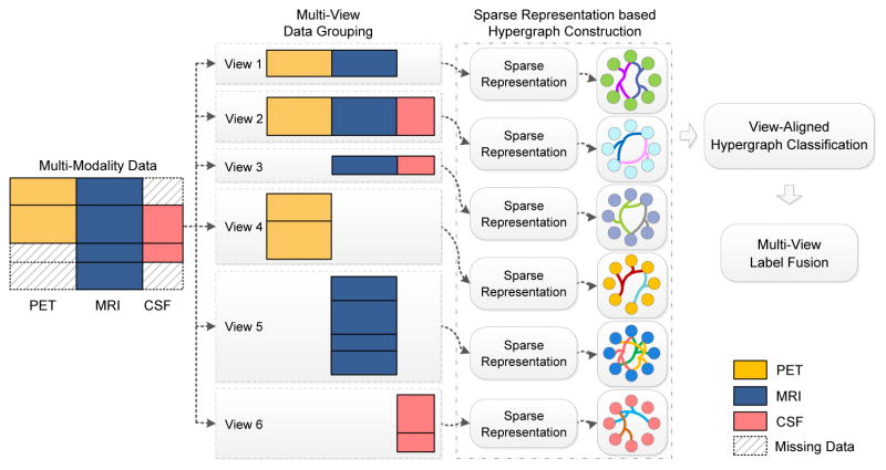
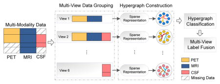
In this paper, we propose a view-aligned hypergraph learning (VAHL) method that utilizes incomplete multi-modality data for AD/MCI diagnosis. Compared with conventional methods, VAHL explicitly incorporates the coherence among views into the learning model, where the optimal weight for each view can also be learned from the data automatically. Figure 1 presents a schematic diagram of the proposed framework using subjects in ADNI-1 database with block-wise missing features (Xiang et al., 2014; Yuan et al., 2012). We first divide the whole data set into M views (M = 6 in Fig. 1) consisting of combinations of modalities. We compute the distances among subjects using a sparse representation model and then construct one hypergraph in each view space. We further propose a view-aligned hypergraph classification model, where the coherence among views is explicitly captured by a proposed view-aligned regularizer. The basic idea of such view-aligned regularizer is that, for one subject represented by two feature vectors in two view spaces, the estimated class labels for such two feature vectors should be similar because they denote the same subject. To arrive at a final classification decision, we agglomerate the class probability scores obtained from different views, via a multi-view label fusion method.
Figure 1.
Illustration of the proposed view-aligned hypergraph learning method, where subjects from the baseline ADNI-1 database are taken as examples. Subjects are divided into M (M = 6 in this study) views according to the data availability of a certain combination of modalities, where each view contains subjects with complete data of combined modalities. We then compute the distances among subjects via a sparse representation model, and construct one hypergraph in each view space. A view-aligned hypergraph classification method is further proposed, followed by a multi-view label fusion method to make a final classification decision.
The rest of the paper is organized as follows. In Section 2, we describe the data used in this study and flesh out the proposed method. In Section 3, we describe the methods used for comparison, the experimental settings, and the experimental results based on the baseline ADNI database (Jack et al., 2008). In Section 4, we investigate the learned weights for different views, the influence of parameters on the classification performance, as well as the influence of the proposed sparse representation based distance measurement for constructing hypergraphs. In Section 5, we conclude this paper and discuss possible future research directions.
2. Material and Method
In this section, we first introduce the database and image pre-processing pipeline used in this study (Section 2.1), and then present the proposed view-aligned hypergraph learning (VAHL) method, which includes multi-view data grouping (Section 2.2), sparse representation based hypergraph construction (Section 2.3), view-aligned hypergraph classification (Section 2.4), and multi-view label fusion (Section 2.5).
2.1. Subjects and Data Pre-Processing
The ADNI-1 database (Jack et al., 2008) is used in this study. According to the Mini-Mental State Examination (MMSE) scores, subjects in ADNI-1 can be divided into three categories: normal control (NC) subjects, MCI subjects, and AD subjects. The general inclusion/exclusion criteria used by ADNI-1 are summarized as follows: 1) NC subjects: Mini-Mental State Examination (MMSE) scores between 24–30 (inclusive), a Clinical Dementia Rating (CDR) of 0, non-depressed, non MCI and non-demented; 2) MCI subjects: MMSE scores between 24–30 (inclusive), a memory complaint, have objective memory loss measured by education adjusted scores on Wechsler Memory Scale Logical Memory II, a CDR of 0.5, absence of significant levels of impairment in other cognitive domains, essentially preserved activities of daily living and an absence of dementia; 3) mild AD: MMSE scores between 20–26 (inclusive), CDR of 0.5 or 1.0 and meets NINCDS/ADRDA criteria for probable AD. In addition, some MCI subjects had converted to AD within 24 months, while some other MCI subjects were stable over time. According to whether MCI subjects would convert to AD within 24 months, the MCI subjects are divided into two categories: 1) stable MCI (sMCI) subjects, if diagnosis was MCI at all available time points (0–96 months); 2) progressive MCI (pMCI) subjects, if diagnosis was MCI at baseline but these subjects converted to AD after baseline within 24 months.
In the baseline ADNI-1 database, there are a total of 807 subjects, including 186 AD subjects, 226 NCs and 395 MCI subjects (consisting of 169 pMCI subjects and 226 sMCI subjects). Detailed description for each category can be found at website1. It is worth noting that all subjects in the baseline ADNI-1 database have T1-weighted structural MRI data, while only 396 subjects have FDG-PET data and 406 subjects have CSF data. The demographic information of the studied subjects (i.e., gender, age, and education) and clinical scores (i.e., MMSE and CDR global) used in this study are summarized in Table 1.
Table 1.
Demographic and clinical information of subjects in the baseline ADNI-1 database
| AD | MCI | NC | |
|---|---|---|---|
| Male/Female | 99/87 | 254/141 | 118/108 |
| Age (Mean ± SD) | 75.40 ± 7.60 | 74.90 ± 7.30 | 76.00 ± 5.00 |
| Edu. (years) (Mean ± SD) | 14.70 ± 3.10 | 15.70 ± 3.00 | 16.00 ± 2.90 |
| MMSE (Mean ± SD) | 23.30 ± 2.00 | 27.00 ± 1.80 | 29.10 ± 1.00 |
| CDR (Mean ± SD) | 0.75 ± 0.25 | 0.50 ± 0.03 | 0.00 ± 0.00 |
Note: Values reported as Mean ± Stand Deviation (SD); MMSE: mini-mental state examination; CDR: Clinical Dementia Rating.
We extract features based on regions-of-interest (ROIs) from MR and PET images. Specifically, for each MR image, we apply the anterior commissure (AC)-posterior commissure (PC) correction using the MIPAV software package2. We then re-sample the images to 256 × 256 × 256 resolution, and apply the N3 algorithm (Sled et al., 1998) to correct intensity in homogeneity. Skull stripping (Wang et al., 2011) is then performed, followed by manual editing to ensure that both skull and dura are cleanly removed. Next, we remove the cerebellum by warping a labeled template to each skull-stripped image. Afterwards, FAST (Zhang et al., 2001) in the FSL software package3 is then applied to segment the human brain into three different tissue types, i.e., gray matter (GM), white matter (WM) and cerebrospinal fluid (CSF). Meanwhile, the anatomical automatic labeling (AAL) atlas (Tzourio-Mazoyer et al., 2002), with 90 pre-defined ROIs in the cerebrum, are aligned to the native space of each subject using a deformable registration algorithm, i.e., HAMMER (Shen and Davatzikos, 2002) that is also extended and applied to other applications (Qiao et al., 2009; Yang et al., 2008; Xue et al., 2006; Verma et al., 2005). Finally, for each subject, we extract the volumes of GM tissue inside those 90 ROIs as features, normalized by the total intracranial volume (estimated by the summation of GM, WM, and CSF volumes from all ROIs). For PET images, we first align each PET image onto its corresponding MR image via a rigid registration, and then compute the mean intensity of each ROI in the PET image as features. In this study, we also employ five CSF biomarkers, including amyloid β (Aβ42), CSF total tau (t-tau), CSF tau hyperphosphorylated at threonine 181 (p-tau), and two tau ratios with respect to Aβ42 (i.e., t-tau/Aβ42 and p-tau/Aβ42). Ultimately, we have a 185-dimensional feature vector for a subject with complete data, including 90 MRI features, 90 PET features and 5 CSF features.
2.2. Multi-View Data Grouping
For subjects with block-wise incomplete MRI, PET and CSF data in the baseline ADNI-1 database, we group them into M(M = 6) views, including “PET+MRI”, “PET+MRI+CSF”, “MRI+CSF”, “PET”, “MRI”, and “CSF”. As shown in Fig. 1, subjects in View 1 have both PET and MRI features, while those in View 6 only have CSF data. In this way, we have complete feature representations for each subject in each view. Using such data grouping strategy, we can make full use of all subjects, without discarding any subjects with missing data or imputing those missing values. Such data grouping method is also used in (Yuan et al., 2012; Xiang et al., 2014) for problems with block-wise incomplete multi-modality data.
The purpose of such multi-view data grouping strategy is to fully utilize all subjects, by grouping them into different views according to the availability of data modalities. Currently, this data grouping approach can only be applied to block-wise incomplete data problem. For more general problems where there may be some missing values in a specific modality for some subjects, we can first impute these missing values using some simple technique (e.g., EM or SVD), and then group subjects into different views.
2.3. Sparse Representation based Hypergraph Construction
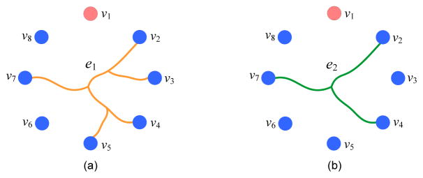
In this study, AD/MCI diagnosis is formulated as a hypergraph based multi-view learning problem. A hypergraph is a generalization of the traditional graph, where each edge (called hyperedge) is a non-empty subset of the vertex set (Zhou et al., 2006; Gao et al., 2012). As shown in Fig. 2(a), the hyperedge e1 contains 5 vertices (i.e., v2, v3, v4, v5, and v7), which demonstrates some high-order relationship among vertices. In contrast, an edge in a conventional graph can only convey the pairwise relationship by connecting only two vertices. For the convenience of presentation, we now introduce some notations for hypergraphs. Throughout the paper, we denote matrices, vectors, and scalars using boldface upper-case letters, boldface lower-case letters, and normal italic letters, respectively. Let 𝒢m = (𝒱, ℰm, wm) denote the m-th hypergraph corresponding to the m-th (m = 1, 2, ···, M) view, where 𝒱 represents the vertex set that contains N vertices, ℰm denotes the hyperedge set, and wm is the weights for hyperedges (with the element representing the weight for the hyperedge ej in the m-th view space). We let represent the number of hyperedges in the m-th hypergraph. Denote as a diagonal matrix of hyperedge weights, i.e., . That is, each diagonal element of Wm denotes the weight for a specific hyperedge in the classification task, with a larger value representing that the hyperedge is more important. Let denote the vertex-hyperedge incidence matrix, with the (vn, ej)-entry indicating whether the vertex vn is connected with other vertices in the hyperedge ej, e.g.,
Figure 2.
Illustration of the proposed hyperedge construction method. Two hyperedges (i.e., e1 and e2) are built by connecting the centroid vertex v1 with the other vertices, according to the sparse representation coefficients obtained by using two l1 regularization parameters.
| (1) |
The degree of a vertex vn is defined as
| (2) |
and the degree for a hyperedge ej is defined as
| (3) |
A key point for hypergraph learning is constructing a set of hyperedges to efficiently model the structure information of data. In conventional methods, the Euclidean distance is generally used to indicate the similarity between pairs of vertices for constructing hyperedges. For instance, in the star expansion method (Zien et al., 1999), we first select each vertex as the centroid vertex, and then construct a hyperedge by connecting this centroid vertex to its s nearest neighbor vertices, where the similarity between two vertices is evaluated by the Euclidean distance. However, the Euclidean distance can only model the local structure information among vertices and does not utilize global information. To address this problem, we propose a sparse representation based distance measurement for hyperedge construction. The reason we utilize sparse representation for computing similarities among vertices is that sparse representation coefficients have proven to be effective in reflecting the global data structure and also robust to data noise (Wright et al., 2009; Qiao et al., 2010).
Given a set of training samples with xn ∈ ℝD, the data matrix X = [x1, x2, ···, xn, ···, xN] ∈ ℝD×N contains N samples in its columns. The goal of sparse representation (Qiao et al., 2010) is to represent each xn using as few samples as possible. Hence, we expect to seek a sparse representation weight vector sn for each xn via the following modified l1 minimization problem
| (4) |
where sn = [sn,1, ···, sn,n−1, 0, sn,n+1, ···, sn,N]⊤ is an N-dimensional vector where the n-th element is equal to zero (implying that xn is removed from X). Note that the element sn,j (j ≠ n) denotes the contribution of xj to the reconstruction of xn. The regularization parameter β is used to control the sparsity of sn, and 1 ∈ RN is a vector of all ones. In Eq. (4), the weight vector ŝn is computed globally in terms of samples from all classes, naturally characterizing the importance of the other samples for the reconstruction of xn. In other words, sample xn is mainly associated with only a few samples with prominent non-zero coefficients in its reconstruction.
With the optimal weight vector ŝn for each xn (n = 1, 2, ···, N) learned from Eq. (4), the sparse representation weight matrix S is defined as
| (5) |
Based on the sparse representation coefficients in Eq. (5), we adopt the star expansion algorithm (Zien et al., 1999) to generate a set of hyperedges. Specifically, in each view space, we first select each vertex as the centroid vertex, and then construct a hyperedge by connecting this centroid vertex to the other vertices, with the sparse representation coefficients as similarity measure. That is, a large coefficient demonstrates a strong connectivity, and a zero coefficient denotes no connectivity. The element of the vertex-hyperedge incidence matrix Hm is defined as
| (6) |
where θ is a small threshold (which is set to 0.001 empirically in this study), and Sn,j is the (n, j)-entry of S in Eq. (5).
It is worth noting that a larger β in Eq. (4) will lead to more zeros in the representation coefficients, which indicates that fewer vertices are used to represent the centroid vertex. In this way, the corresponding hyperedge would contain less vertices, demonstrating a relatively local data structure. To model multi-scale structure information of data, we propose to employ multiple (e.g., q) values for β to construct multiple sets of hyperedges. As illustrated in Fig. 2, we construct two hyperedges (i.e., e1 and e2) by connecting a centroid vertex v1 with the other vertices, where each hyperedge corresponds to a specific β. For the hypergraph 𝒢m in the m-th view space, we can finally obtain hyperedges in the vertex-hyperedge incidence matrix Hm. In this way, we can obtain hundreds of hyperedges, some of which may not be informative enough for subsequent classification model. We further propose to learn optimal weights for hyperedges in Section 2.4.2 in order to identify those most informative hyperedges.
2.4. View-Aligned Hypergraph Classification
In the following, we first propose a view-aligned regularizer to explicitly model the underlying coherence among views, and then develop a view-aligned hypergraph classification model as well as an efficient alternating optimization algorithm.
2.4.1. View-Aligned Regularizer
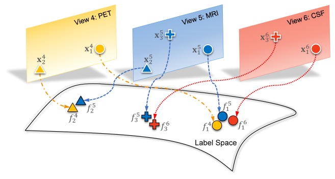
Denote fm ∈ ℝN as the class probability score vector for N subjects in the m-th view, and F = [f1, f2, ···, fm, ···, fM] ∈ ℝN×M, where M is the number of views. The proposed view-aligned regularizer is illustrated in Fig. 3, where different colors and shapes denote different views and subjects, respectively. For instance, circles represent a subject having PET (View 4), MRI (View 5) and CSF (View 6) data, that are denoted as and , respectively. Intuitively, after being mapped into the label space, their estimated class probability scores (i.e., , and ) should be close to each other, since they represent the same subject. Similarly, for the subject with only PET and MRI features (i.e., triangles for and ), the distance between and should be small in the label space. Denote Ωm ∈ ℝN×N as a diagonal matrix, with the diagonal element if the n-th subject has missing values in the m-th view, and , otherwise. Then, the proposed view-aligned regularizer is defined as
Figure 3.
Illustration of the proposed view-aligned regularizer. Circle, cross and triangle represent three subjects, respectively. Yellow, blue, and red denote the views of “PET”, “MRI”, and “CSF”, respectively.
| (7) |
Let represent the vertex degree matrix whose diagonal entries correspond to the degree of each vertex. Denote as the hyperedge degree matrix, with diagonal elements representing the degree of each hyperedge. The hypergraph regularization term (Zhou et al., 2006) is defined as
| (8) |
where Lm = I − Θm is the hypergraph Laplacian matrix, I is an identity matrix, and .
2.4.2. View-Aligned Hypergraph Classification
Denote y = [(yla)⊤, (yun)⊤]⊤ ∈ ℝN, where yla denotes label information for labeled data and yun represents label information for unlabeled data. For the n-th sample, yn = 1 if it is associated with the positive class (e.g., AD), yn = −1 if it belongs to the negative class (e.g., NC), and yn = 0 if its category is unknown. Since different views and hyperedges may play different roles in a classification task, it is intuitively reasonable to learn weights for different views and for hyperedges from data. Denote α ∈ ℝM as a weight vector, with its element αm representing the weight for the m-th view. Denote the Frobenius norm of the matrix Wm as . In this study, we resort to the multi-task learning framework (Argyriou et al., 2008) for classification, and regard the classification in each view space as a specific learning task. The proposed view-aligned hypergraph classification (VAHC) model is formulated as
| (9) |
where the first term is the empirical loss, and the second one is the hypergraph Laplacian regularizer (Zhou et al., 2006). It is worth noting that the third term in Eq. (9) is the proposed view-aligned regularizer, encouraging the similarity of the estimated class labels for one subject represented in two different views. The last term and those constraints in Eq. (9) are used to penalize the complexity of the weights (i.e., Wm) for hyperedges and also the weights (i.e., α) for views. The regularization parameter (αm)2 is used to prevent the degenerate solution of α. In addition, μ and λ are regularization parameters for our proposed view-aligned regularizer and the hyperedge weight regularizer, respectively. With Eq. (9), one can jointly learn the class probability scores F, the optimal weights for different views (i.e., α), and the optimal weights for hyperedges (i.e., ) from data.
Since the problem in Eq. (9) is not jointly convex with respect to F, α, and , we adopt an alternating optimization method to solve the proposed objective function. Specifically, in the first step, we aim to optimize F with fixed α and . In such case, the objective function in Eq. (9) can be written as
| (10) |
The partial derivative of the objective function in Eq. (10) with respect to fm is as follows
| (11) |
| (12) |
In the second step, given fixed F and α, we can optimize . Then, the objective function in Eq. (9) can be re-written as follows
| (13) |
The partial derivative of Eq. (13) with respect to Wm is as follows
| (14) |
| (15) |
where , and is an identity matrix.
In the third step, we optimize α with fixed F and , and the problem in Eq. (9) can be re-written as follows
| (16) |
The partial derivative of Eq. (16) with respect to αm is as follows
| (17) |
| (18) |
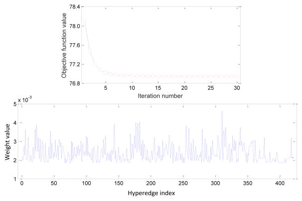
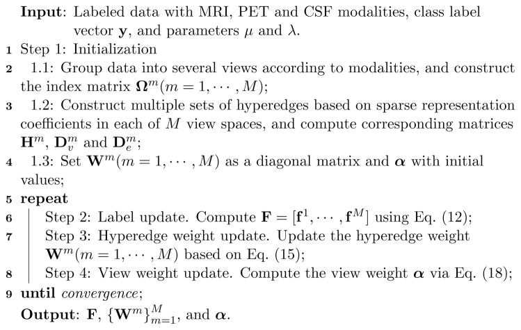
The alternating optimization process is repeated until convergence. The entire process of the above-mentioned method is summarized in Algorithm 1. In Fig. 4, we plot the change of the objective function values of Eq. (9) using different iteration numbers and the learned weights for hyperedges in the AD vs. NC classification, with μ = 10 and λ = 10 for illustration. From Fig. 4 (top), it can be seen that the objective function value decreases rapidly within 5 iterations, illustrating the fast convergence of the proposed optimization algorithm. Figure 4 (bottom) shows that the learned weights for different hyperedges vary significantly, implying that many hyperedges could be less discriminative in reflecting the true structure of data. In such a case, learning the optimal weights from data, as we do in this study via Eq. (9), provides an efficient way to suppress the contribution of hyperedges that are less important.
Figure 4.
Objective function values with respect to different iterations (top), and the learned weights for hyperedges (bottom) in AD vs. NC classification, with μ = 10 and λ = 10.
Algorithm 1.
View-aligned hypergraph classification
2.5. Multi-View Label Fusion
For a new testing sample z, we now compute the weighted mean of its class probability scores for making a final classification decision. Specifically, its class label can be obtained via
| (19) |
where , and αm is the optimal weight of the m-th view learned from VAHC defined in Eq. (9).
It is worth noting that if z has missing values in a specific modality, the weights for related views associated with this modality will be 0. For instance, the weights for the views of “PET+MRI+CSF”, “MRI+CSF” and “CSF” will be zeros if there are missing CSF data in the testing sample z.
3. Results
Here, we present the competing methods (Section 3.1) and experimental settings (Section 3.2), followed by experimental results of our method in comparison to baseline methods (Section 3.3) and several state-of-the-art methods (Section 3.4). We further compare the computational costs of different methods in Section 3.5.
3.1. Methods for Comparison
We first compare the proposed VAHL method with four baseline approaches based on data imputation techniques, including 1) Zero (missing values filled with zeros), 2) k-Nearest Neighbor (KNN) (Hastie et al., 1999; Troyanskaya et al., 2001; Hastie et al., 2005), 3) Expectation Maximization (EM) (Schneider, 2001), and 4) Singular Value Decomposition (SVD) (Golub and Reinsch, 1970). Assuming that the feature values are collected in the form of a matrix (as shown in Fig. 1), four baseline imputation-based methods are briefly summarized below.
1) In Zero method, missing values are filled with zeros. If data are normalized to have a mean of zero and unit standard deviation, this method is equivalent to the mean-value imputation method. That is, the missing feature values are filled with the means of corresponding feature values available in the same row.
2) In KNN method (Hastie et al., 1999; Troyanskaya et al., 2001), each missing value is filled with the weighted mean of its k-nearest neighbor columns. Specifically, we first adopt KNN to identify the feature columns that are most similar to the one with missing values. Those missing values are then filled in with the weighted mean of the values in the neighbor columns. Following (Thung et al., 2014), the weight for a specific neighbor column is inversely proportional to the Euclidean distance between the neighbor column and the column with missing values.
3) In EM method (Schneider, 2001), missing values are imputed using the EM algorithm. Specifically, in the E step, we estimate the mean and the covariance matrix from the feature matrix, with missing values filled with the estimates from the previous E step (or initialized as zeros). In the M step, we assign the conditional expectation values to the missing elements based on the available values, the estimated mean, and the covariance. Next, we re-estimate the mean and the covariance according to the filled feature matrix. These two steps are repeated until convergence.
4) In SVD method (Golub and Reinsch, 1970), missing values are iteratively filled-in using the matrix completion technique with low-rank approximation. That is, some initial guesses (e.g., zeros) are first assigned to the missing values and the method of SVD is then adopted to obtain a low-rank approximation of a filled-in matrix. Next, we update the missing elements with their corresponding values in the low-rank estimation matrix. Then, we perform SVD to the updated matrix again, and such processes are repeated until convergence.
The proposed VAHL method is further compared with six state-of-the-art methods: 1) two Ensemble based methods (Ingalhalikar et al., 2012) using weighted average (denoted as Ensemble-1) and average (denoted as Ensemble-2) strategies, respectively; 2) two incomplete multi-source feature (iMSF) learning methods (Yuan et al., 2012) with square loss (denoted as iMSF-1) and logistic loss (denoted as iMSF-2); 3) an incomplete source-feature selection (iSFS) method (Xiang et al., 2014); and 4) a matrix shrinkage and completion (MSC) method (Thung et al., 2014).
1) In the Ensemble based method (Ingalhalikar et al., 2012), an ensemble classification technique is adopted to fuse multiple classifiers by using different subsets of samples with complete data. Specifically, this method first divides the data into different subsets, and then selects relevant features using signal-to-noise ratio coefficient filter algorithm (Guyon and Elisseeff, 2003). Based on the selected features, a linear discriminant analysis (LDA) (Scholkopft and Mullert, 1999) classifier is constructed for each subset, followed by the fusion of classification results of multiple LDA classifiers to make a final decision for a testing subject. According to different fusion strategies, there are two versions of this method. The first one, denoted as Ensemble-1, is based on weighted averaging, where each classifier is assigned a specific weight based on its classification error on the training data. In the second approach (i.e., Ensemble-2), all classifiers are assigned equal weights.
2) The iMSF method (Yuan et al., 2012) is a multi-view based method. Similar to our data grouping technique, iMSF first partitions subjects into several views, and a specific classifier is constructed in each view. A structural sparse learning model is then developed to select a common set of features among these tasks. Finally, an ensemble model is used to combine all models together. There are two versions of iMSF based on different loss functions, i.e., the least square loss (denoted as iMSF-1) and the logistic loss (denoted as iMSF-2).
3) As another multi-view based method, iSFS (Xiang et al., 2014) first partitions subjects into several views according to the availability of data modalities. A bi-level (i.e., both feature-level and view-level) feature learning model is proposed to learn the optimal weights for both features and views.
4) The MSC method (Thung et al., 2014) is a matrix completion based method. In MSC, the feature and the target output matrices are first combined into a large matrix that are partitioned into smaller sub-matrices, and each sub-matrix consists of samples with complete features (corresponding to a certain combination of modalities) and target outputs. A multi-task sparse learning method is applied to select informative features and samples, resulting in a shrunk version of the original matrix. The missing features and unknown target outputs of the shrunk matrix is then completed simultaneously, by using an EM imputation method (Schneider, 2001) or a fixed-point continuation method (Ma et al., 2011).
3.2. Experimental Settings
In the experiments, we perform four classification tasks, including AD vs. NC, pMCI vs. NC, MCI vs. NC, and pMCI vs. sMCI classification. A 10-fold cross-validation strategy is used for performance evaluation. Specifically, all subjects are partitioned into 10 subsets with roughly equal size. Each time one subset is designated as the testing data and the rest subsets as the training data. This process is repeated 10 times to avoid any bias introduced by random partitioning of the data, and finally the mean classification results are reported.
We adopt seven metrics for performance evaluation, including the classification accuracy (ACC), sensitivity (SEN), specificity (SPE), balanced accuracy (BAC), positive predictive value (PPV), negative predictive value (NPV) and the area under the receiver operating characteristic curve (AUC) (Fletcher et al., 2012). Denote TP, TN, FP and FN as true positive, true negative, false positive and false negative, respectively. These evaluation metrics are defined as: ACC=(TP+TN)/(TP+TN+FP+FN), SEN=TP/(TP+FN), SPE=TN/(TN+FP), BAC=(SEN+SPE)/2, PPV=TP/(TP+FP), and NPV=TN/(TN+FN).
To optimize the parameters for different methods, we further perform an inner 10-fold cross-validation using the training data. That is, each training subset is further divided into 10 subsets for cross-validation parameter selection (Xiang et al., 2014). The parameters in Eq. (9) (i.e., μ and λ) are chosen from {10−3, 10−2, ···, 104}, while the iteration number in the proposed alternating optimization algorithm for Eq. (9) is empirically set to 20. Multiple parameter values for β in Eq. (4) are set to [10−3, 10−2, 10−1, 100] for constructing multiple sets of hyperedges for each hypergraph (w.r.t. each view) in VAHL. The parameter k for KNN is chosen from {3, 5, 7, 9, 11, 15, 20}, the rank parameter is chosen from {5, 10, 15, 20, 25, 30} for SVD, and the parameter λ for iMSF is chosen from {10−5, 10−4, ···, 101}.
3.3. Comparison with Baseline Methods
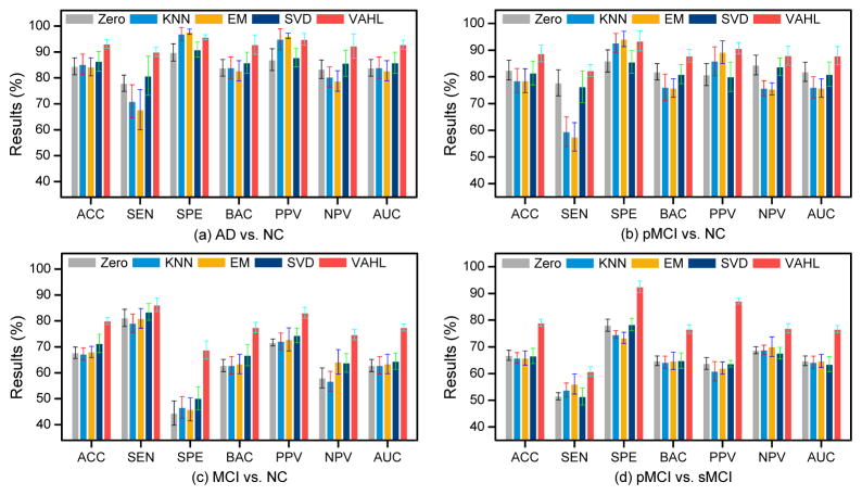
We first compare VAHL with imputation methods, including Zero, KNN (Hastie et al., 1999; Troyanskaya et al., 2001), EM (Schneider, 2001) and SVD (Golub and Reinsch, 1970). In Fig. 5, we report mean results as well as standard deviations achieved by different methods in four classification tasks, i.e., AD vs. NC, pMCI vs. NC, MCI vs. NC, and pMCI vs. sMCI classification. From Fig. 5, we can observe that VAHL consistently outperforms those four baseline methods in terms of seven evaluation criteria.
Figure 5.
Comparison between the proposed VAHL method and four baseline methods in four classification tasks.
3.4. Comparison with State-of-the-art Methods
We further compare VAHL with several state-of-the-art methods, including Ensemble-1 and Ensemble-2 (Ingalhalikar et al., 2012), iMSF-1 and iMSF-2 (Yuan et al., 2012), iSFS (Xiang et al., 2014), and MSC (Thung et al., 2014). It is worth noting that iSFS first selects informative features from the original feature space, and then utilizes Random Forest classifier for classification. MSC utilizes matrix completion technique to simultaneously impute those missing values and unknown target outputs. The results for four classification tasks are reported in Table 2 and Table 3, where the best results are marked in boldface. In these tables, results of iSFS (Xiang et al., 2014) and MSC (Thung et al., 2014) are directly taken from their respective papers. From these two tables, we can observe that, in AD vs. NC, pMCI vs. NC, MCI vs. NC and pMCI vs. sMCI classification, our VAHL method generally outperforms the other methods in terms of ACC, SEN, SPE and AUC. For instance, in AD vs. NC classification, VAHL achieves a 4.6% improvement in terms of ACC compared with other methods. It is worth noting that both iSFS and VAHL learn the optimal weights for different views from data. Table 2 shows that, compared with iSFS, VAHL achieves much better results in AD vs. NC classification, and comparable results in pMCI vs. NC classification. The improvements given by VAHL can be attributed to the capability in modeling coherence among different views.
Table 2.
Comparison with the state-of-the-art methods in AD vs. NC and pMCI vs. NC classification
| Method | AD vs. NC | pMCI vs. NC | ||||||
|---|---|---|---|---|---|---|---|---|
|
| ||||||||
| ACC (%) | SEN (%) | SPE (%) | AUC (%) | ACC (%) | SEN (%) | SPE (%) | AUC (%) | |
| Ensemble-1 | 83.03 | 78.54 | 86.72 | 89.82 | 73.92 | 71.61 | 75.58 | 78.88 |
| Ensemble-2 | 81.07 | 76.37 | 84.94 | 87.39 | 71.14 | 68.08 | 73.33 | 74.98 |
| iMSF-1 | 86.41 | 76.91 | 94.24 | 85.57 | 82.53 | 69.32 | 92.11 | 80.71 |
| iMSF-2 | 86.97 | 75.78 | 93.90 | 86.34 | 83.29 | 71.37 | 92.11 | 81.74 |
| iSFS | 88.48 | 88.95 | 88.16 | 88.56 | 89.86 | 99.15 | 84.00 | 91.57 |
| MSC | 88.50 | 83.70 | 92.70 | 94.40 | - | - | - | - |
| VAHL | 93.10 | 90.00 | 95.65 | 94.83 | 89.95 | 89.35 | 93.48 | 92.00 |
Table 3.
Comparison with the state-of-the-art methods in MCI vs. NC and pMCI vs. sMCI classification
| Method | MCI vs. NC | pMCI vs. sMCI | ||||||
|---|---|---|---|---|---|---|---|---|
|
| ||||||||
| ACC (%) | SEN (%) | SPE (%) | AUC (%) | ACC (%) | SEN (%) | SPE (%) | AUC (%) | |
| Ensemble-1 | 62.58 | 65.42 | 57.73 | 64.40 | 68.10 | 55.44 | 77.77 | 64.60 |
| Ensemble-2 | 61.61 | 64.16 | 57.28 | 62.07 | 65.56 | 51.15 | 75.41 | 61.78 |
| iMSF-1 | 70.64 | 81.62 | 54.42 | 63.02 | 65.82 | 56.90 | 72.38 | 68.20 |
| iMSF-2 | 71.61 | 82.83 | 54.73 | 63.78 | 64.55 | 56.85 | 70.22 | 66.00 |
| MSC | 71.50 | 75.30 | 64.90 | 77.30 | - | - | - | - |
| VAHL | 80.00 | 86.19 | 68.78 | 80.49 | 79.00 | 60.80 | 92.53 | 79.66 |
We further use the McNemars test (Dietterich, 1998) to assess whether the difference in performance between our proposed method and each competing method is significant, with the corresponding p-values reported in Table 4. These results show that our proposed method performs significantly better than the compared methods, as demonstrated by very small p-values (< 0.001).
Table 4.
The p-values in the McNemars test between the performances of the proposed method and each competing method in four classification tasks
| Method | AD vs. NC | pMCI vs. NC | MCI vs. NC | pMCI vs. sMCI |
|---|---|---|---|---|
| Zero | 0.0016 | 0.0021 | 0.0019 | 0.0030 |
| KNN | 0.0014 | 0.0026 | 0.0013 | 0.0033 |
| EM | 0.0028 | 0.0024 | 0.0017 | 0.0031 |
| SVD | 0.0027 | 0.0020 | 0.0024 | 0.0035 |
| Ensemble-1 | 0.0038 | 0.0039 | 0.0011 | 0.0028 |
| Ensemble-2 | 0.0032 | 0.0035 | 0.0013 | 0.0022 |
| iMSF-1 | 0.0040 | 0.0042 | 0.0022 | 0.0023 |
| iMSF-2 | 0.0039 | 0.0043 | 0.0020 | 0.0019 |
3.5. Computational Costs
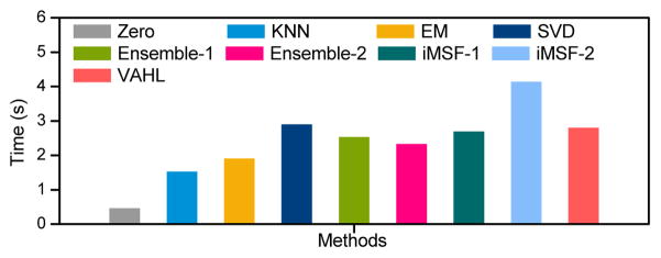
Figure 6 lists the computational costs of different methods in AD vs. NC classification. As shown in Fig. 6, the computational cost of VAHL is less than that of iMSF-2, and is comparable to SVD and iMSF-1. Compared with Zero, KNN, and EM methods, VAHL needs more computational time, due to the time spent on the construction of multiple hypergraphs. Overall, the computational cost of our method is reasonable and acceptable in practical applications.
Figure 6.
Run time comparison between the proposed VAHL method and competing methods in AD vs. NC classification.
4. Discussion
We first investigate the optimal weights for different views learned from our proposed VAHC model in Section 4.1, and then evaluate the influence of two regularization parameters in Eq. (9) in Section 4.2. In Section 4.3, we study the influence of different similarity measurement for hyperedge construction, including the proposed sparse representation and conventional Euclidean distance based measurements. We also study the influence of the proposed view-centralized regularizer on the learning performance in Section 4.4. In Section 4.5, we further show the results using complete data in the ADNI-1 database.
4.1. Learned Weights for Different Views
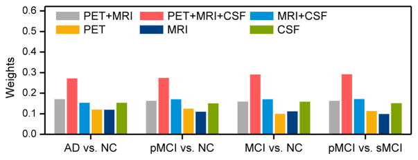
Now we show the optimal weights for different views learned from the proposed VAHC model defined in Eq. (9), with results given in Fig. 7. From Fig. 7, we can observe that the weights for the view of “PET+MRI+CSF” are much larger than those of the other five views in four classification tasks. This indicates that the view that contains the combination of MRI, PET, and CSF data can provide more discriminative information, compared with the other views. Among three views that contain only one single modality data, Fig. 7 indicates that the weights for the view of “CSF” are generally larger than those for the views of “MRI” and “PET”. This implies that CSF could be comparatively more effective biomarkers in distinguishing AD/MCI patients from the whole population, compared with MRI and PET data.
Figure 7.
Optimal weights of different views (i.e., “PET+MRI”, “PET+MRI+CSF”, “MRI+CSF”, “PET”, “MRI”, and “CSF”) learned from the proposed view-aligned hypergraph classification model in four classification tasks.
4.2. Influence of Regularization Parameters
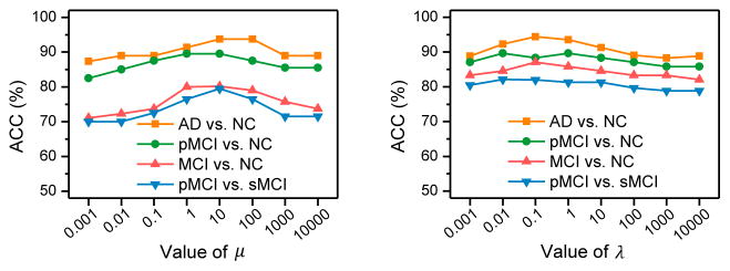
In the proposed classification model in Eq. (9), there are two parameters (i.e., μ and λ) for our proposed view-aligned regularizer and the hyperedge weight regularizer, respectively. We have evaluated the influences of those two regularization parameters on the performance of our method, with results shown in Fig. 8. The values of μ and λ are varied within {10−3, 10−2, ···, 104}. From Fig. 8, we can observe we can observe that, with different values of μ and λ, the classification accuracies fluctuate in a large range. For instance, as shown in Fig. 8 (left), VAHL generally achieves better results in terms of ACC when 1 ≤ μ ≤ 10. Also, Fig. 8 (right) indicates that the best results are usually obtained by VAHL using 0.1 ≤ λ ≤ 1 in four classification tasks. These results imply that the proposed view-aligned regularizer and the hypergraph Laplacian regularizer play important roles in the VAHC model.
Figure 8.
Influence of the parameters (i.e.. μ and λ) on the proposed method.
4.3. Sparse Representation Coefficients vs. Euclidean Distance
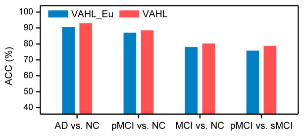
We further compare VAHL (using a sparse representation based hypergraph construction approach) with the conventional method (denoted as VAHL_Eu) that uses the Euclidean distance as similarity measurement for constructing a hypergraph in each view space. For fair comparison, in VAHL_Eu, multiple neighbors are used for constructing hyperedges via the star expansion algorithm (Zien et al., 1999), where each centroid vertex is connected with its s-nearest neighbors. In the experiments, we adopt the neighbor size s = [3, 5, 7, 9, 11, 15] for VAHL_Eu. Figure 9 reports the classification accuracies achieved by VAHL and VAHL_Eu. From this figure, we can observe that VAHL consistently outperforms VAHL_Eu in four classification tasks. This demonstrates that, for hypergraph construction, the use of sparse representation brings performance improvement compared with that of the Euclidean distance. This can partly contribute to the global structure information conveyed by sparse representation coefficients (Wright et al., 2009).
Figure 9.
Comparison between VAHL and VAHL_Eu. Here, VAHL and VAHL_Eu denote the proposed methods that adopt sparse representation coefficients and Euclidean distance as similarity measurements for constructing hyperedges, respectively.
4.4. Influence of the View-Aligned Regularizer
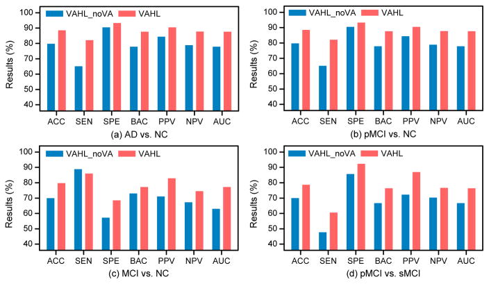
We also study the influence of the proposed view-aligned regularizer on the classification performance. We denote “VAHL_noVA” as the VAHL model without the view-aligned regularizer (i.e., μ = 0 in Eq. 9), and perform experiments to compare VAHL and VAHL_noVA (with results shown in Fig. 10). It can be seen from Fig. 10 that VAHL outperforms VAHL_noVA in terms of accuracy in four classification tasks, implying that modeling the coherence among views via the proposed view-aligned regularizer can boost the classification performance of hypergraph based model.
Figure 10.
Comparison between VAHL and VAHL_noVA. Here, VAHL_noVA denotes the proposed VAHL model without the view-aligned regularizer.
4.5. Complete Data vs. Incomplete Data
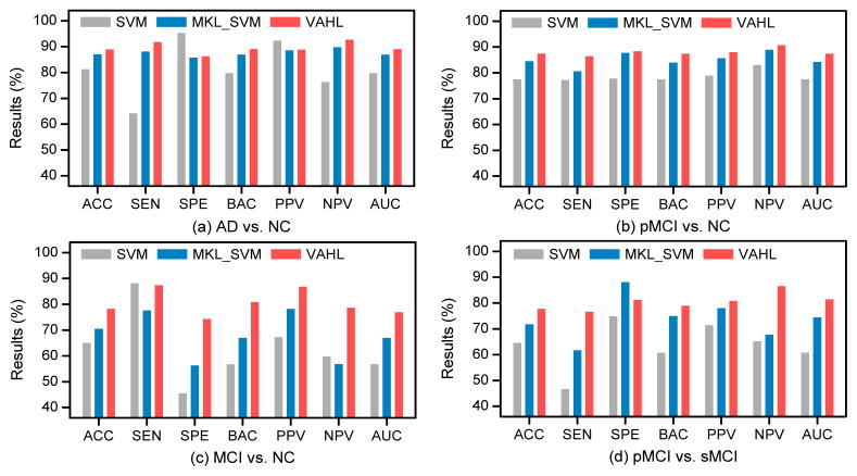
We further investigate whether methods using incomplete data can boost the learning performance, compared with those using only complete data (with PET, MRI, and CSF features). In the baseline ADNI-1 database, there are a total of 202 subjects that have complete data, including 51 AD, 42 pMCI, 57 sMCI, and 52 NC subjects. We compare the proposed VAHL method with both SVM and multi-kernel SVM (MKL_SVM) (Zhang et al., 2011) using complete data, with corresponding results shown in Fig. 11. Here, the concatenation of MRI, PET, and CSF features is used in SVM, while each of three data modalities is treated as a specific kernel in MKL_SVM. It is worth noting that our VAHL model has only one view (i.e., “PET+MRI+CSF”) in the case of using complete data. From Fig. 11 and Fig. 5, we can observe that the overall performance of methods using complete data is worse than that of the method using incomplete data, suggesting that utilizing more data can promote the AD/MCI diagnosis performance. Also, it can be seen from Fig. 11 that VAHL generally outperforms the conventional SVM and MKL_SVM, demonstrating that our method provides a better way to utilize multi-modality data for AD/MCI diagnosis.
Figure 11.
Classification results achieved by different methods using complete data, where MLK_SVM denotes multi-kernel SVM.
5. Conclusions
In this paper, we propose a view-aligned hypergraph learning (VAHL) method using incomplete multi-modality data for AD/MCI diagnosis. Specifically, we first partition the original data into several views according to the availability of data modalities, and construct one hypergraph in each view using a sparse representation based hypergraph construction approach. We then develop a view-aligned hypergraph classification model to explicitly capture the underlying coherence among views, as well as automatically learn the optimal weights of different views from data. A multi-view label fusion method is employed to assemble the estimated class probability scores to arrive at a final classification decision. Results on the baseline ADNI-1 database (with MRI, PET, and CSF modalities) demonstrate the efficacy of our method in AD/MCI diagnosis. In this study, we employ all original features for hypergraph construction, while there may exist noisy or redundant information in original features. It is interesting to select those most informative features for subsequent hypergraph construction, which will be part of our future work. Also, we only perform experiments on the baseline ADNI-1 database with three data modalities. As a future work, we will evaluate the proposed method on more datasets, such as the ADNI-2 database and the dataset in the Computer-Aided Diagnosis of Dementia (CADDementia) challenge (Bron et al., 2015).
Highlights.
We developed a new hypergraph learning model to capture the coherence among views;
We proposed a sparse representation based hypergraph construction method;
We designed a multi-view label fusion method for making classification decisions.
Acknowledgments
This study was supported by NIH grants (EB006733, EB008374, EB009634, MH100217, AG041721, AG042599, AG010129, and AG030514).
Data used in preparation of this article were obtained from the Alzheimer’s Disease Neuroimaging Initiative (ADNI) database. As such, the investigators within the ADNI contributed to the design and implementation of ADNI and/or provided data but did not participate in analysis or writing of this report. A complete listing of ADNI investigators can be found online4.
Footnotes
Publisher's Disclaimer: This is a PDF file of an unedited manuscript that has been accepted for publication. As a service to our customers we are providing this early version of the manuscript. The manuscript will undergo copyediting, typesetting, and review of the resulting proof before it is published in its final citable form. Please note that during the production process errors may be discovered which could affect the content, and all legal disclaimers that apply to the journal pertain.
References
- Argyriou A, Evgeniou T, Pontil M. Convex multi-task feature learning. Machine Learning. 2008;73:243–272. [Google Scholar]
- Association A, et al. 2013 Alzheimer’s disease facts and figures. Alzheimer’s & Dementia. 2013;9:208–245. doi: 10.1016/j.jalz.2013.02.003. [DOI] [PubMed] [Google Scholar]
- Bron EE, Smits M, Van Der Flier WM, Vrenken H, Barkhof F, Scheltens P, Papma JM, Steketee RM, Orellana CM, Meijboom R, et al. Standardized evaluation of algorithms for computer-aided diagnosis of dementia based on structural MRI: The CADDementia challenge. NeuroImage. 2015;111:562–579. doi: 10.1016/j.neuroimage.2015.01.048. [DOI] [PMC free article] [PubMed] [Google Scholar]
- Brookmeyer R, Johnson E, Ziegler-Graham K, Arrighi HM. Forecasting the global burden of Alzheimer’s disease. Alzheimer’s & Dementia. 2007;3:186–191. doi: 10.1016/j.jalz.2007.04.381. [DOI] [PubMed] [Google Scholar]
- Chetelat G, Desgranges B, De La Sayette V, Viader F, Eustache F, Baron JC. Mild cognitive impairment can FDG-PET predict who is to rapidly convert to Alzheimer’s disease? Neurology. 2003;60:1374–1377. doi: 10.1212/01.wnl.0000055847.17752.e6. [DOI] [PubMed] [Google Scholar]
- Cuingnet R, Gerardin E, Tessieras J, Auzias G, Lehéricy S, Habert MO, Chupin M, Benali H, Colliot O. Automatic classification of patients with Alzheimer’s disease from structural MRI: A comparison of ten methods using the ADNI database. NeuroImage. 2011;56:766–781. doi: 10.1016/j.neuroimage.2010.06.013. [DOI] [PubMed] [Google Scholar]
- Dietterich TG. Approximate statistical tests for comparing supervised classification learning algorithms. Neural Computation. 1998;10:1895–1923. doi: 10.1162/089976698300017197. [DOI] [PubMed] [Google Scholar]
- Fletcher RH, Fletcher SW, Fletcher GS. Clinical Epidemiology: The Essentials. Lippincott Williams & Wilkins; 2012. [Google Scholar]
- Foster NL, Heidebrink JL, Clark CM, Jagust WJ, Arnold SE, Barbas NR, DeCarli CS, Turner RS, Koeppe RA, Higdon R. FDG-PET improves accuracy in distinguishing frontotemporal dementia and Alzheimer’s disease. Brain. 2007;130:2616–2635. doi: 10.1093/brain/awm177. [DOI] [PubMed] [Google Scholar]
- Gao Y, Wang M, Tao D, Ji R, Dai Q. 3-D object retrieval and recognition with hypergraph analysis. IEEE Transactions on Image Processing. 2012;21:4290–4303. doi: 10.1109/TIP.2012.2199502. [DOI] [PubMed] [Google Scholar]
- Golub GH, Reinsch C. Singular value decomposition and least squares solutions. Numerische Mathematik. 1970;14:403–420. [Google Scholar]
- Guyon I, Elisseeff A. An introduction to variable and feature selection. The Journal of Machine Learning Research. 2003;3:1157–1182. [Google Scholar]
- Hansson O, Zetterberg H, Buchhave P, Londos E, Blennow K, Minthon L. Association between CSF biomarkers and incipient Alzheimer’s disease in patients with mild cognitive impairment: A follow-up study. The Lancet Neurology. 2006;5:228–234. doi: 10.1016/S1474-4422(06)70355-6. [DOI] [PubMed] [Google Scholar]
- Hastie T, Tibshirani R, Friedman J, Franklin J. The elements of statistical learning: Data mining, inference and prediction. The Mathematical Intelligencer. 2005;27:83–85. [Google Scholar]
- Hastie T, Tibshirani R, Sherlock G, Eisen M, Brown P, Botstein D. Imputing Missing Data for Gene Expression Arrays. 1999. [Google Scholar]
- Herholz K, Salmon E, Perani D, Baron J, Holthoff V, Frölich L, Schönknecht P, Ito K, Mielke R, Kalbe E. Discrimination between Alzheimer dementia and controls by automated analysis of multicenter FDG PET. NeuroImage. 2002;17:302–316. doi: 10.1006/nimg.2002.1208. [DOI] [PubMed] [Google Scholar]
- Ingalhalikar M, Parker WA, Bloy L, Roberts TP, Verma R. Medical Image Computing and Computer-Assisted Intervention–MICCAI 2012. Springer; 2012. Using multiparametric data with missing features for learning patterns of pathology; pp. 468–475. [DOI] [PMC free article] [PubMed] [Google Scholar]
- Jack CR, Bernstein MA, Fox NC, Thompson P, Alexander G, Harvey D, Borowski B, Britson PJ, Whitwell LJ, Ward C. The Alzheimer’s disease neuroimaging initiative (ADNI): MRI methods. Journal of Magnetic Resonance Imaging. 2008;27:685–691. doi: 10.1002/jmri.21049. [DOI] [PMC free article] [PubMed] [Google Scholar]
- Kawarabayashi T, Younkin LH, Saido TC, Shoji M, Ashe KH, Younkin SG. Age-dependent changes in brain, CSF, and plasma amyloid β protein in the tg2576 transgenic mouse model of Alzheimer’s disease. The Journal of Neuroscience. 2001;21:372–381. doi: 10.1523/JNEUROSCI.21-02-00372.2001. [DOI] [PMC free article] [PubMed] [Google Scholar]
- Liu M, Zhang D, Shen D. Relationship induced multi-template learning for diagnosis of Alzheimer’s disease and mild cognitive impairment. IEEE Transactions on Medical Imaging. 2016;35:1463–1474. doi: 10.1109/TMI.2016.2515021. [DOI] [PMC free article] [PubMed] [Google Scholar]
- Ma S, Goldfarb D, Chen L. Fixed point and bregman iterative methods for matrix rank minimization. Mathematical Programming. 2011;128:321–353. [Google Scholar]
- Qiao H, Zhang H, Zheng Y, Ponde DE, Shen D, Gao F, Bakken AB, Schmitz A, Kung HF, Ferrari VA, et al. Embryonic stem cell grafting in normal and infarcted myocardium: Serial assessment with MR imaging and PET dual detection. Radiology. 2009;250:821–829. doi: 10.1148/radiol.2503080205. [DOI] [PMC free article] [PubMed] [Google Scholar]
- Qiao L, Chen S, Tan X. Sparsity preserving projections with applications to face recognition. Pattern Recognition. 2010;43:331–341. [Google Scholar]
- Reiman EM, Langbaum JB, Tariot PN. Alzheimer’s prevention initiative: A proposal to evaluate presymptomatic treatments as quickly as possible. Biomarkers in Medicine. 2010;4:3–14. doi: 10.2217/bmm.09.91. [DOI] [PMC free article] [PubMed] [Google Scholar]
- Schneider T. Analysis of incomplete climate data: Estimation of mean values and covariance matrices and imputation of missing values. Journal of Climate. 2001;14:853–871. [Google Scholar]
- Scholkopft B, Mullert KR. Fisher discriminant analysis with kernels. Neural Networks for Signal Processing IX. 1999;1:1. [Google Scholar]
- Shen D, Davatzikos C. HAMMER: Hierarchical attribute matching mechanism for elastic registration. IEEE Transactions on Medical Imaging. 2002;21:1421–1439. doi: 10.1109/TMI.2002.803111. [DOI] [PubMed] [Google Scholar]
- Sled JG, Zijdenbos AP, Evans AC. A nonparametric method for automatic correction of intensity nonuniformity in MRI data. IEEE Transactions on Medical Imaging. 1998;17:87–97. doi: 10.1109/42.668698. [DOI] [PubMed] [Google Scholar]
- Thung KH, Wee CY, Yap PT, Shen D. Neurodegenerative disease diagnosis using incomplete multi-modality data via matrix shrinkage and completion. NeuroImage. 2014;91:386–400. doi: 10.1016/j.neuroimage.2014.01.033. [DOI] [PMC free article] [PubMed] [Google Scholar]
- Troyanskaya O, Cantor M, Sherlock G, Brown P, Hastie T, Tibshirani R, Botstein D, Altman RB. Missing value estimation methods for DNA microarrays. Bioinformatics. 2001;17:520–525. doi: 10.1093/bioinformatics/17.6.520. [DOI] [PubMed] [Google Scholar]
- Tzourio-Mazoyer N, Landeau B, Papathanassiou D, Crivello F, Etard O, Delcroix N, Mazoyer B, Joliot M. Automated anatomical labeling of activations in SPM using a macroscopic anatomical parcellation of the MNI MRI single-subject brain. NeuroImage. 2002;15:273–289. doi: 10.1006/nimg.2001.0978. [DOI] [PubMed] [Google Scholar]
- Verma R, Mori S, Shen D, Yarowsky P, Zhang J, Davatzikos C. Spatiotemporal maturation patterns of murine brain quantified by diffusion tensor MRI and deformation-based morphometry. Proceedings of the national academy of sciences of the United States of America. 2005;102:6978–6983. doi: 10.1073/pnas.0407828102. [DOI] [PMC free article] [PubMed] [Google Scholar]
- Wang Y, Nie J, Yap PT, Shi F, Guo L, Shen D. Medical Image Computing and Computer-Assisted Intervention–MICCAI 2011. Springer; 2011. Robust deformable-surface-based skull-stripping for large-scale studies; pp. 635–642. [DOI] [PubMed] [Google Scholar]
- Wolz R, Julkunen V, Koikkalainen J, Niskanen E, Zhang DP, Rueckert D, Soininen H, Lötjönen J. Multi-method analysis of MRI images in early diagnostics of Alzheimer’s disease. PLOS ONE. 2011;6:e25446. doi: 10.1371/journal.pone.0025446. [DOI] [PMC free article] [PubMed] [Google Scholar]
- Wright J, Yang AY, Ganesh A, Sastry SS, Ma Y. Robust face recognition via sparse representation. IEEE Transactions on Pattern Analysis and Machine Intelligence. 2009;31:210–227. doi: 10.1109/TPAMI.2008.79. [DOI] [PubMed] [Google Scholar]
- Xiang S, Yuan L, Fan W, Wang Y, Thompson PM, Ye J. Bi-level multi-source learning for heterogeneous block-wise missing data. NeuroImage. 2014;102:192–206. doi: 10.1016/j.neuroimage.2013.08.015. [DOI] [PMC free article] [PubMed] [Google Scholar]
- Xue Z, Shen D, Karacali B, Stern J, Rottenberg D, Davatzikos C. Simulating deformations of MR brain images for validation of atlas-based segmentation and registration algorithms. NeuroImage. 2006;33:855–866. doi: 10.1016/j.neuroimage.2006.08.007. [DOI] [PMC free article] [PubMed] [Google Scholar]
- Yang J, Shen D, Davatzikos C, Verma R. International Conference on Medical Image Computing and Computer-Assisted Intervention. Springer; 2008. Diffusion tensor image registration using tensor geometry and orientation features; pp. 905–913. [DOI] [PubMed] [Google Scholar]
- Yuan L, Wang Y, Thompson PM, Narayan VA, Ye J. Multi-source feature learning for joint analysis of incomplete multiple heterogeneous neuroimaging data. NeuroImage. 2012;61:622–632. doi: 10.1016/j.neuroimage.2012.03.059. [DOI] [PMC free article] [PubMed] [Google Scholar]
- Zhang D, Wang Y, Zhou L, Yuan H, Shen D. Multimodal classification of Alzheimer’s disease and mild cognitive impairment. NeuroImage. 2011;55:856–867. doi: 10.1016/j.neuroimage.2011.01.008. [DOI] [PMC free article] [PubMed] [Google Scholar]
- Zhang J, Gao Y, Gao Y, Munsell B, Shen D. Detecting anatomical landmarks for fast Alzheimer’s disease diagnosis. IEEE Transactions on Medical Imaging. 2016 doi: 10.1109/TMI.2016.2582386. [DOI] [PMC free article] [PubMed] [Google Scholar]
- Zhang Y, Brady M, Smith S. Segmentation of brain MR images through a hidden Markov random field model and the expectation-maximization algorithm. IEEE Transactions on Medical Imaging. 2001;20:45–57. doi: 10.1109/42.906424. [DOI] [PubMed] [Google Scholar]
- Zhou D, Huang J, Schölkopf B. Learning with hypergraphs: Clustering, classification, and embedding. Advances in Neural Information Processing Systems. 2006:1601–1608. [Google Scholar]
- Zien JY, Schlag MD, Chan PK. Multilevel spectral hypergraph partitioning with arbitrary vertex sizes. IEEE Transactions on Computer-Aided Design of Integrated Circuits and Systems. 1999;18:1389–1399. [Google Scholar]


