Significance
Working memory (WM) is a core cognitive function thought to rely on persistent activity patterns in populations of neurons in prefrontal cortex (PFC), yet the neural circuit mechanisms remain unknown. Single-neuron activity in PFC during WM is heterogeneous and strongly dynamic, raising questions about the stability of neural WM representations. Here, we analyzed WM activity across large populations of neurons in PFC. We found that despite strong temporal dynamics, there is a population-level representation of the remembered stimulus feature that is maintained stably in time during WM. Furthermore, these population-level analyses distinguish mechanisms proposed by theoretical models. These findings inform our fundamental understanding of circuit mechanisms underlying WM, which may guide development of treatments for WM impairment in brain disorders.
Keywords: working memory, prefrontal cortex, population coding
Abstract
Working memory (WM) is a cognitive function for temporary maintenance and manipulation of information, which requires conversion of stimulus-driven signals into internal representations that are maintained across seconds-long mnemonic delays. Within primate prefrontal cortex (PFC), a critical node of the brain’s WM network, neurons show stimulus-selective persistent activity during WM, but many of them exhibit strong temporal dynamics and heterogeneity, raising the questions of whether, and how, neuronal populations in PFC maintain stable mnemonic representations of stimuli during WM. Here we show that despite complex and heterogeneous temporal dynamics in single-neuron activity, PFC activity is endowed with a population-level coding of the mnemonic stimulus that is stable and robust throughout WM maintenance. We applied population-level analyses to hundreds of recorded single neurons from lateral PFC of monkeys performing two seminal tasks that demand parametric WM: oculomotor delayed response and vibrotactile delayed discrimination. We found that the high-dimensional state space of PFC population activity contains a low-dimensional subspace in which stimulus representations are stable across time during the cue and delay epochs, enabling robust and generalizable decoding compared with time-optimized subspaces. To explore potential mechanisms, we applied these same population-level analyses to theoretical neural circuit models of WM activity. Three previously proposed models failed to capture the key population-level features observed empirically. We propose network connectivity properties, implemented in a linear network model, which can underlie these features. This work uncovers stable population-level WM representations in PFC, despite strong temporal neural dynamics, thereby providing insights into neural circuit mechanisms supporting WM.
The neuronal basis of working memory (WM) in prefrontal cortex (PFC) has been studied for decades through single-neuron recordings from monkeys performing tasks in which a transient sensory stimulus must be held in WM across a seconds-long delay to guide a future response. These studies discovered that a key neural correlate of WM in PFC is stimulus-selective persistent activity, i.e., stable elevated firing rates in a subset of neurons, that spans the delay (1). These neurophysiological findings have grounded a leading hypothesis that WM is supported by stable persistent activity patterns in PFC that bridge the gap between stimulus and response epochs. Because the timescales of WM maintenance (several seconds) are longer than typical timescales of neuronal and synaptic integration (10–100 ms), mechanisms at the level of neural circuits may be critical for generating WM activity in PFC (2). A leading theoretical framework proposes that PFC circuits subserve WM maintenance through dynamical attractors, i.e., stable fixed points in network activity, generated by strong recurrent connectivity (3, 4).
Recent neurophysiological studies have called into question whether WM activity in PFC can be appropriately understood in terms of persistent activity and attractor dynamics. These studies highlight the high degree of heterogeneity and strong temporal dynamics in single-neuron responses during WM (5, 6), rather than temporally constant activity patterns. Because only a small proportion of WM-related PFC neurons show well-tuned, stable persistent activity, attractor dynamics may not be the dominant form of WM coding. Researchers have emphasized alternative forms of population coding, specifically dynamic coding, in which the mnemonic representation shifts over time during WM maintenance (7, 8). In turn, such observations have motivated theoretical proposals for alternative neural circuit mechanisms for WM that produce dynamical and heterogeneous activity (9, 10).
These studies centralize a tension between temporal dynamics and stable coding of stimulus features during WM maintenance. In high-dimensional state spaces of network activity, however, it is possible for heterogeneous neuronal dynamics to coexist with a stable population coding for WM within a specific subspace (11). Whether dynamic activity in PFC supports a robust stable population coding for WM remains unclear. Furthermore, dynamic coding raises the challenge of how WM information in PFC can be robustly read out through plausible neurobiological mechanisms, because a subspace corresponds to a set of readout weights (12).
To investigate these issues, we applied population-level analyses to two large datasets of single-neuron spike trains recorded in PFC, from two seminal WM tasks: the oculomotor delayed response (ODR) task (13, 14) and the vibrotacticle delayed discrimination (VDD) task (15). In both tasks, PFC populations exhibit strong temporal dynamics during WM, yet there exists a subspace, identifiable via principal component analysis (PCA), in which mnemonic representations are coded stably in time. This mnemonic subspace supports decoding throughout WM, performing comparably to dynamic coding subspaces. We found that population measures dissociate among mechanisms in three previously proposed WM circuit models. Key features of the PFC data are not captured by these three models, yet they are by a simple subspace attractor model. Taken together, our findings demonstrate a stable and robust population coding for WM in PFC and pose constraints for circuit mechanisms supporting WM.
Results
Tasks and Datasets.
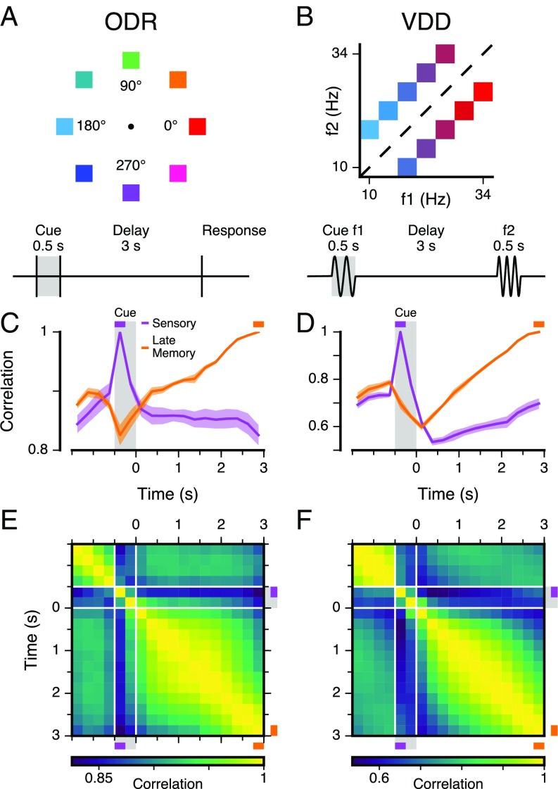
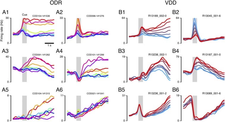
The ODR and VDD tasks share common features, facilitating comparison across datasets. Both tasks demand parametric WM of an analog stimulus variable: visuospatial angle for ODR and vibrotactile frequency for VDD (Fig. 1 A and B). Both tasks have a 0.5-s cue epoch followed by a 3-s delay epoch, which is relatively long and allows characterization of time-varying WM representations. The tasks also contrast in several features, allowing us to test the generality of our findings. They differ in stimulus modality (visual for ODR vs. somatosensory for VDD), role of WM in guiding behavioral response (veridical report of location for ODR vs. binary discrimination for VDD), and prototypical stimulus tuning curves of single PFC neurons (bell shaped for ODR vs. monotonic for VDD). Each dataset, collected by a different laboratory, contains spike trains from hundreds of single neurons (645 for ODR; 479 for VDD) recorded from the lateral PFC of two macaque monkeys (14, 15). To minimize bias in characterizing population activity, neurons were not preselected for tuning properties. We used a pseudopopulation approach to study the state–space dynamics of population activity (8, 12, 16, 17), rather than the properties of the heterogenous individual neurons (Figs. S1 and S2). The activity of neurons corresponds to a vector in an -dimensional space, with each dimension representing the firing rate of one neuron. The time-varying population activity for each stimulus condition thereby corresponds to a trajectory within this space.
Fig. 1.
WM tasks and PFC population dynamics. (A) In the ODR task, the subject fixates on a central point, and a visuospatial cue of variable spatial angle is presented for 0.5 s, followed by a 3-s mnemonic delay. After the delay, the subject makes a saccadic eye movement to the remembered location (14). (B) In the VDD task, the subject receives a 0.5-s vibrotactile stimulus of variable mechanical frequency (cue, f1) to the finger, followed by a 3-s mnemonic delay. After the delay, a second stimulus (f2) is presented and the subject reports, by level release, which stimulus had a higher frequency (15). (C and D) Correlation between population states as a function of time, within the same stimulus condition. The sensory state is defined by the first 0.25 s of the cue epoch and the late memory state by the last 0.25 s of the delay epoch. Colored shaded regions mark SEM. (E and F) Correlation between the population states at different timepoints (i.e., time-lagged autocorrelation). The correlation between states is generally high due to a broad distribution of overall firing rates across neurons (Fig. S2). The traces in C and D are slices along the corresponding timepoint.
Fig. S1.
Example single neurons, for ODR (A1–A6) and VDD (B1–B6) datasets, highlighting the heterogeneity and temporal dynamics in single-neuron activity in PFC during WM encoding and maintenance. Plotted is the PSTH for each stimulus condition, with trace colors marking the different stimulus conditions corresponding to those shown in the task schematics of Fig. 1. The gray shaded region marks the cue epoch. Purely for visualization of example single-neuron activity in this figure only, PSTHs were smoothed using PCA, which denoises across PSTH traces rather than only over time. For all reported results, activity is not smooth in any way except for binning in 0.25-s time bins.
Fig. S2.
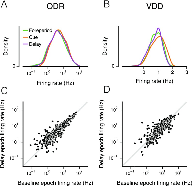
Distribution of mean firing rates across neurons in different task epochs. (A and B) Firing-rate distributions plotted in a lin-log plot, with logarithmic x axis and linear y axis. The observed distribution of firing rates is approximately a log-normal distribution. Interestingly, when compared across task epochs (foreperiod, cue, working memory delay), the overall distribution of firing rates does not change substantially. In particular, the distribution during the delay epoch is essentially the same as during the foreperiod. (C and D) Correlation across neurons of mean firing rates between task epochs. Shown here are the correlations between delay epoch and the foreperiod epoch. The values of the Pearson’s r correlation coefficient of the log-transformed firing rates are the following: For ODR, 0.88 for foreperiod–cue, 0.91 for foreperiod–delay, and 0.89 for cue–delay; for VDD, 0.75 for foreperiod–cue, 0.83 for foreperiod–delay, and 0.66 for cue–delay.
Population Dynamics.
We first examined the dynamics of population activity during WM by characterizing the similarity of activity patterns between two timepoints. We calculated the correlation, across neurons, between the population state at one timepoint and the state at another timepoint, within a stimulus condition (18). Fig. 1 C and D shows the time course of this similarity for two reference timepoints: a “sensory” state during the cue epoch and a “late memory” state at the end of the delay epoch. Fig. 1 E and F shows the population correlation across all timepoints. For both datasets, WM activity patterns in PFC exhibit strong temporal dynamics with the population state changing strongly throughout the cue and delay epochs. The strength of these dynamics can be observed in the late memory trace (Fig. 1 C and D): The correlation for early in the delay is as low as it is for the foreperiod. These temporal dynamics at the population level are consistent with prior characterizations of delay dynamics at the single-neuron level (5, 6). We note that trial averaging could obscure dynamics (e.g., oscillations) that are not phase locked to task timing.
Stable Coding in a Mnemonic Subspace.
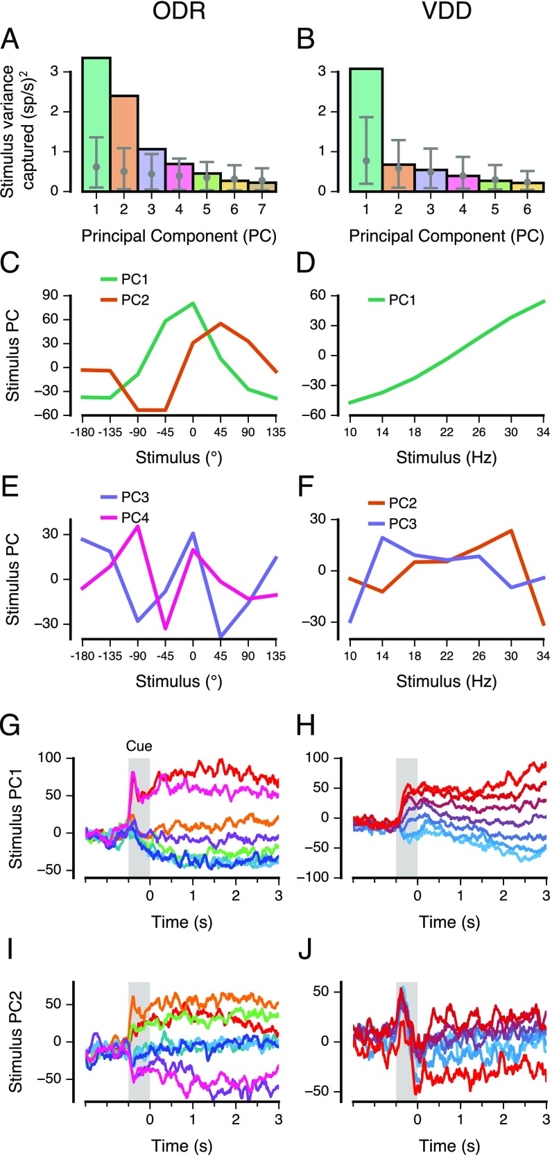
Are these strong population dynamics compatible with stable coding for WM? In the state–space framework, stable mnemonic coding corresponds to a fixed subspace within which the neural trajectories during WM are relatively time invariant and separable across stimulus conditions. To test this hypothesis, we sought to define and characterize a mnemonic coding subspace. There are a variety of dimensionality reduction methods to define candidate coding subspaces. Motivated by the neurobiological relevance of a mnemonic subspace, which may provide representations for downstream readout of WM, we sought to define a subspace that can be plausibly learned for readout via known forms of synaptic plasticity. There is an established theoretical literature linking Hebbian learning to dimensionality reduction via PCA (19–21). We therefore applied PCA to the time-averaged delay activity across stimulus conditions (SI Text) (Fig. S3). The leading principal axes, ranked by variance captured, define a -dimensional linear subspace, which we denote the mnemonic subspace, which lies closest on average to the datapoints. Because this subspace is defined by time-averaged activity, our approach does not explicitly use timing information (as in ref. 16). A primary rationale is that if a subspace is accessible through time-insensitive PCA, then it can potentially be learned neurally through Hebbian plasticity.
Fig. S3.
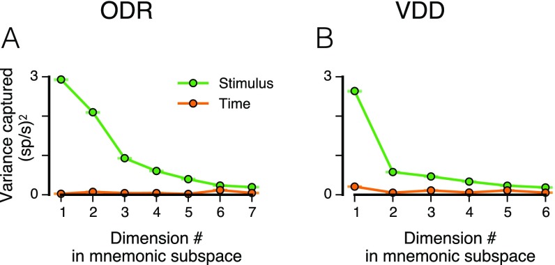
PCA of time-averaged delay activity. (A and B) Amount of stimulus variance captured by each principal axis, for time-averaged delay activity. The number of PCs is one fewer than the number of stimulus conditions. Stimulus variance captured is normalized by the number of neurons. Gray error bars show the mean and central 95% bounds, calculated through shuffling the stimulus identities of trials. For the ODR dataset, a subspace defined by the first two principal axes captures 68% of the stimulus variance. For the VDD dataset, a subspace defined by the first principal axis captures 60% of the stimulus variance. (C and D) Leading PCs, i.e., projections of the time-averaged delay activity along the leading principal axes (2 for ODR, 1 for VDD). For ODR (C), PC1 and PC2 provide quasi-sinusoidal coding of stimuli. For VDD (D), PC1 provide quasi-linear coding of stimuli. (E and F) Projections along the next two leading principal axes. (G and H) Population trajectory projected along principal axis 1, showing relative stability of stimulus coding during the delay epoch as well as in the preceding cue epoch. (I and J) Population trajectory projected along principal axis 2.
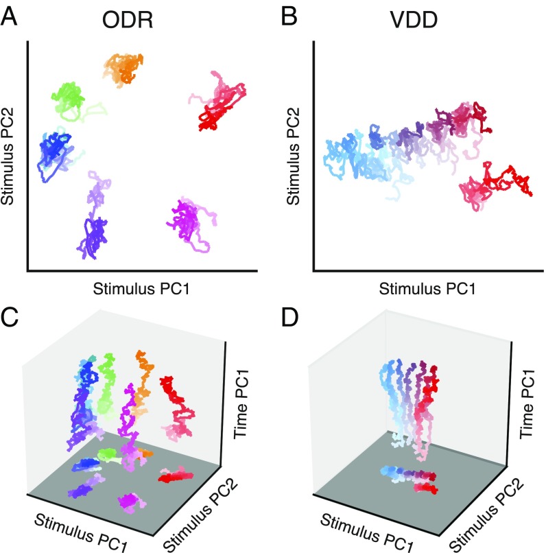
Surprisingly, we found that when the neural trajectories are projected into the mnemonic subspace, the resulting delay activity is remarkably stable in time, even though this subspace is not designed to minimize temporal variation (Fig. 2 A and B). Separation and stability of trajectories can be quantified and compared through the across-condition stimulus variance and within-condition time variance (Fig. S4). For ODR, the first two principal components (PCs) of the mnemonic subspace (i.e., the projections of the activity along the corresponding principal axes) largely reflect the horizontal and vertical stimulus dimensions (Fig. 2A and Fig. S3C). For the leftmost three locations, traces overlap in the PC1–PC2 subspace but are distinguishable in higher PCs (Fig. S3 E and F). This compressed representation of the ipsilateral (left) visual hemifield is expected due to the prominent contralateral bias for coding of visual space in PFC (13, 22). For VDD, the first PC of the mnemonic subspace provides a monotonic, quasi-linear ordering of the cue stimulus frequency (Fig. 2B and Fig. S3D). To visualize population temporal dynamics in relation to the mnemonic subspace, we constructed 3D projections. In Fig. 2 C and D, the x and y axes show the first two PCs of the mnemonic subspace. The z axis is an orthogonal axis in the state space that captures a large amount of time variance during the delay. Mnemonic subspace trajectories vary in time more for VDD than for ODR, exhibiting a gradual increase in separation during the delay. As this view shows, WM activity undergoes strong changes over time without interfering with coding that is stable and separable within the mnemonic subspace.
Fig. 2.
Stable population coding of WM coexists with strong temporal dynamics. (A and B) Population trajectories during the WM delay epoch projected into the mnemonic subspace, defined via PCA on time-averaged delay activity. Here the x and y axes show the first and second principal components (PC1 and PC2) of the subspace. Each trace corresponds to a stimulus condition, colored as in Fig. 1 A and B. The shading of the traces marks the time during the delay, from early (light) to late (dark). (C and D) Three-dimensional projections, illustrating the strong temporal dynamics coexisting with stable coding in the mnemonic subspace. The x and y axes are as in A and B. The z axis (time PC1) is an orthogonal axis in the state space that captures time-related activity variance, but does not indicate time explicitly. Within each plot, all axes are scaled equally.
Fig. S4.
Stimulus- and time-related variance of delay activity captured by the mnemonic subspace, for each dimension in the mnemonic subspace. (A and B) The green points show the variance (per neuron), across stimuli, for the time-averaged mean delay activity, i.e., . The orange points show the average within-stimulus, time-related variance (per neuron) of the trajectory (using 0.25-s time bins), i.e., . The orange points may overestimate the true time-related variance, as variance will be contributed by noisy estimation of the PSTH due to finite numbers of trials. Error bars denote the 95% range generated by leave-one-neuron-out jackknife resampling, characterizing how much these estimates would change if additional neurons were included.
Stable and Dynamic Coding.
We have shown that the PCA-defined mnemonic subspace captures a relatively stable stimulus representation throughout the WM delay. However, this subspace may not capture components of the WM representation that are highly dynamic during the delay. In a dynamic coding scenario, a fixed subspace would fail to capture much stimulus variance, because stimulus representations change over time, and a “dynamic” subspace that is reoptimized for each timepoint would capture a much larger amount of stimulus variance. To characterize the relative strengths of stable and dynamic coding, we measured the amount of stimulus variance captured by a given subspace (i.e., the resulting firing-rate variance across stimuli when the population activity, at a given timepoint, is projected into the subspace), for the mnemonic subspace as well as for a dynamic subspace that is redefined for each timepoint by the same PCA method. To allow proper comparison between mnemonic and dynamic subspaces, we applied a split-data approach for cross-validation and used equal amounts of training data (SI Text).
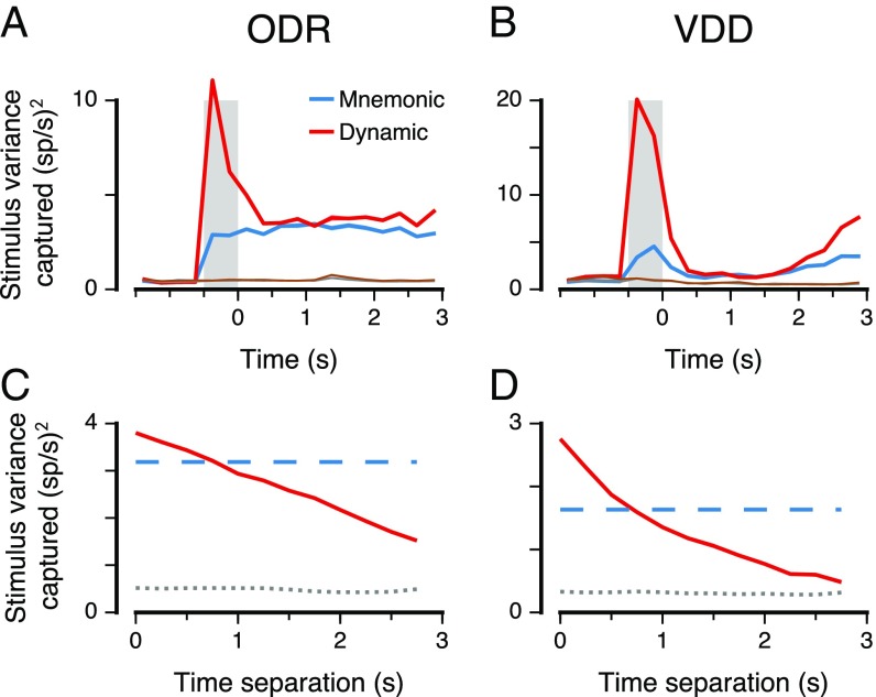
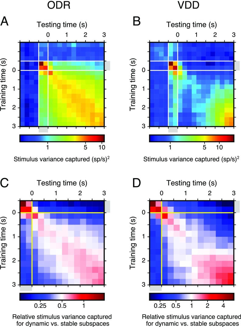
We found that the mnemonic and dynamic subspaces capture significantly more stimulus variance than expected by chance for all timepoints across the cue and delay epochs (, t test) (Fig. 3 A and B). The mnemonic subspace encodes a comparable amount of variance across the cue and delay epochs, even though it was defined using only delay-epoch data, suggesting that mnemonic coding begins early during stimulus presentation. Relative to the mnemonic subspace, the dynamic subspace captures a comparable amount of stimulus variance during the delay, but substantially more during the cue. This suggests a separate sensory representation that is activated during stimulus presentation. For VDD but not ODR, the variance increases substantially toward the end of the delay, due to dynamic coding as well as increased separation within the mnemonic subspace, which could potentially be due to task differences in response type. We tested generalizability of the dynamic subspace by measuring how well the subspace defined at one timepoint captures stimulus variance in activity at a different timepoint. The amount of variance captured decays smoothly with increasing separation between these two timepoints (Fig. 3 C and D and Fig. S5), reflecting the timescales over which dynamic coding evolves. For zero time separation, the dynamic subspace captures more variance on average than the mnemonic subspace, but for all separations greater than 0.5 s, the mnemonic subspace captures more variance, showing robustness of stable coding in this subspace.
Fig. 3.
Stimulus variance captured by the mnemonic and dynamic coding subspaces. The mnemonic subspace is defined using delay activity as in Fig. 2. The dynamic subspace is defined from data for each timepoint (0.25 s). The dimensionality of the subspaces is 2 for ODR (A and C) and 1 for VDD (B and D), matching the dimensionality of the stimulus feature for each task. (A and B) Stimulus variance captured for stable mnemonic subspace (blue) and for a dynamic subspace optimized for each timepoint (red). Chance values for the stable (gray) and dynamic (brown) subspaces were calculated by shuffling stimulus trial labels. (C and D) Generalizability of the dynamic subspace across time. The red curve marks the stimulus variance captured by the dynamic subspace defined at one time for activity at another time separated by a given time separation, averaged across timepoints during the delay. The blue dashed line marks the stimulus variance captured by the mnemonic subspace, averaged across the delay epoch. The gray dotted line marks the mean chance level during the delay. Shaded bands mark SEM.
Fig. S5.
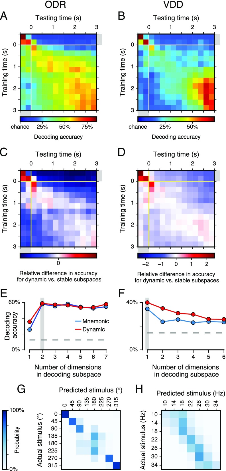
Stimulus variance captured by mnemonic and dynamic subspaces and generalizability of the dynamic subspace. (A and B) Stimulus variance captured by the dynamic subspace as a function of the training timepoint and testing point. That is, activity at the training time is used to define the dynamic subspace, and the activity at the testing time is projected into that subspace. The diagonal elements, when training time and testing time are the same, are plotted in the Fig. 3 A and B. (C and D) The relative difference in stimulus variance captured for dynamic vs. mnemonic subspaces ( and , respectively), as a function of training time and testing time during the cue and delay epochs. That is, the value plotted is . Red (blue) regions show where the dynamic subspace has higher (lower) stimulus variance captured than the mnemonic subspace. These results show that the dynamic subspace classifier does not generalize well, so that for off-diagonal elements when training time and testing time are separated by more than 0.5 s, the mnemonic subspace shows greater performance. This characterizes the timescales of dynamic coding. Color bars have a logarithmic scale.
Decoding.
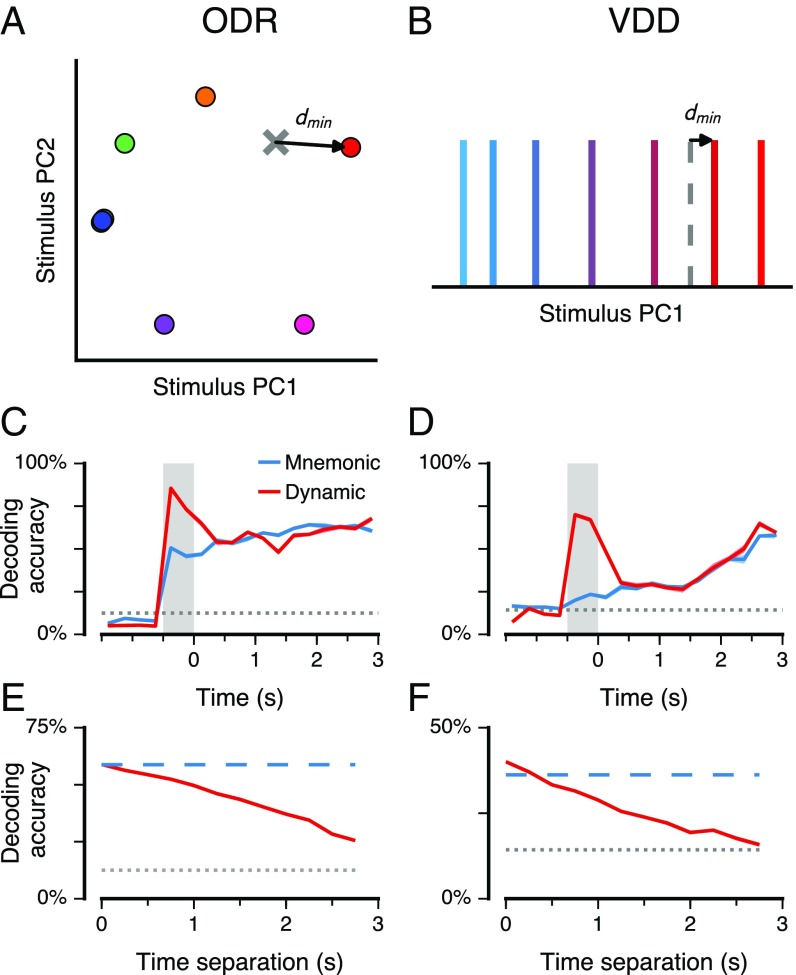
The above findings do not directly test whether the stimulus can be reliably decoded from neural activity. Even within a fixed subspace, representations could potentially rearrange within the subspace across time. To explicitly quantify decoding accuracy from the mnemonic and dynamic subspaces, we designed a neurobiologically plausible decoder based on the nearest-centroid classifier (SI Text). This simple classifier has a straightforward neural interpretation: winner-take-all selection following readout from the low-dimensional linear readout weights defining the subspace. We reserve the spike counts for a given timepoint from a single trial, for leave-one-out cross-validation. We construct decoding subspaces, mnemonic and dynamic, as well as the centroids related to each stimulus condition in those subspaces, using equal amounts of training data from the other trials. The classifier choice is given by the stimulus condition whose centroid is nearest to the test datapoint (Fig. 4 A and B).
Fig. 4.
Decoding of stimulus via stable and dynamic coding subspaces. (A and B) Schematic of the subspace decoder. Activity at a given timepoint for a single trial is projected into the subspace, and the classifier’s winner-take-all readout is the stimulus condition whose centroid is nearest (). As in Fig. 3, the number of dimensions used for the subspace is 2 for ODR and 1 for VDD. (C and D) Decoding accuracy over time for the mnemonic (blue) and dynamic (red) coding subspaces. Chance performance for the stable (gray) and dynamic (brown) subspaces was calculated by shuffling stimulus trial labels. (E and F) Generalizability of the dynamic subspace across time. The red curve marks the stimulus variance captured by the dynamic subspace defined at one time for activity at another time separated by a given time separation, averaged across timepoints during the delay. The blue dashed line marks the stimulus variance captured by the mnemonic subspace, averaged across the delay epoch. The gray dotted line marks chance performance. Shaded bands mark SEM.
We found that the mnemonic subspace yielded decoding performance that is above chance during the delay epoch and during the cue epoch (, t test), even though the subspace was trained using only delay-epoch data (Fig. 4 C and D and Fig. S6). Both subspaces produced comparable performance during the delay epoch. Errors in the mnemonic subspace were typically made to similar stimulus conditions (Fig. S6). Relative to mnemonic, the dynamic decoder performed substantially better during the cue and early delay. As with variance captured (Fig. 3B), for VDD decoding improves in the late delay. For some timepoints the dynamic decoder performed slightly worse than the mnemonic decoder, potentially due to noisy subspace estimation from limited trials. We tested generalizability across time of the dynamic subspace classifier (Fig. 4 E and F and Fig. S6) and found a gradual decay in performance with increasing time separation, consistent with prior studies (7, 8). Compared with mnemonic, the dynamic decoder had marginally higher decoding performance at zero time separation, but substantially lower performance when applied to separations greater than 0.5 s.
Fig. S6.
Decoding performance for a nearest-mean classifier based on mnemonic or dynamic subspaces. (A and B) Decoding accuracy and generalizability of the dynamic subspace classifier as a function of the training timepoint and testing point. The diagonal elements, when training time and testing time are the same, are plotted in Fig. 4 B and C. (C and D) The relative difference in stimulus variance captured for dynamic vs. mnemonic subspaces ( and , respectively), as a function of training time and testing time during the cue and delay epochs. That is, the value plotted is . Red (blue) regions show where the dynamic subspace has higher (lower) decoding accuracy than the mnemonic subspace. These results show that the dynamic subspace outperforms the mnemonic subspace most during the cue and early delay epochs. Furthermore, the dynamic subspace classifier does not generalize well, so that for off-diagonal elements when training time and testing time are separated by more than 0.5 s, the mnemonic subspace shows greater performance. (E and F) Decoding accuracy as a function of the number of dimensions included in the decoding subspace. A -dimensional decoding subspace is defined by the leading principal components. The gray dashed lines mark chance performance. In C and D the gray shaded line marks the number of dimensions used for each dataset, 2 for ODR and 1 for VDD, which matches the dimensionality of the stimulus. The decoding accuracy can plateau or decline with increasing dimensionality, because adding another dimension not only increases signal but also increases trial-by-trial variability that can impair classifier performance. (G and H) Confusion matrix characterizing the pattern of errors made by the mnemonic subspace classifier. The confusion matrix shows the distribution of classifier predictions for the stimulus condition (columns) for each actual stimulus condition (rows). For both ODR and VDD, the classification errors (off-diagonal elements of the confusion matrix) are primarily made to stimuli that are near actual stimulus. (G) For ODR, most errors are due to the compressed representation of ipsilateral space, which produces poor separation among the three left hemifield stimuli (135°, 180°, and 225°). (H) For VDD, most errors are to adjacent stimuli, and the predicted stimulus is biased toward more central stimulus values.
Neural Circuit Models.
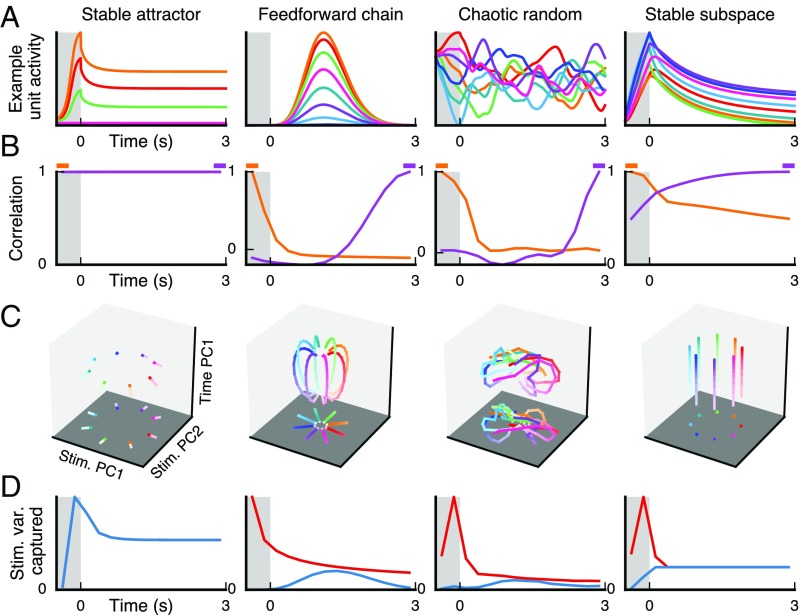
What implications do these findings have for the neural circuit mechanisms supporting WM activity in PFC? To investigate this, we applied the same population-level analyses to four theoretical models of neural WM circuits. We first analyzed three previously proposed circuit models (SI Text). The first model, denoted as a “stable attractor” network, uses strong recurrent excitation and lateral inhibition to maintain a stimulus-selective persistent activity pattern as a stable fixed point of the network dynamics (3, 23). The second model is denoted as a “feedforward chain” network (9). In contrast to the recurrent excitation in the stable attractor model, this network has a feedforward chain structure of excitatory connections, and information is encoded only transiently in each neuron. In the third model, denoted as a “chaotic random” network, recurrent connections are random but strong, placing the network dynamics in a chaotic regime (10, 24). Stimulus presentation temporarily suppresses chaotic activity, allowing the network to reliably encode the stimulus (25). During the delay, the network activity evolves chaotically from this stimulus-selective point, generating activity patterns that are distinguishable across stimuli but with representations that change over time. We found that none of these models captured key features of WM population coding observed in the PFC datasets (Fig. 5 A–D, Leftmost three columns). The stable attractor model exhibits stable coding in the mnemonic subspace, but not strong temporal dynamics, because network activity is at a fixed point during the delay. In contrast, the feedforward chain and chaotic random models exhibit strong temporal dynamics, but both fail to exhibit stable coding in the mnemonic subspace, because WM representations change throughout the delay.
Fig. 5.
Population-level analyses measures distinguish theoretical model network mechanisms for population coding and dynamics. We tested four dynamical circuit models, described in the main text: stable attractor, feedforward chain, chaotic random, and stable subspace. The simulated stimulus features are designed to match the ODR task. (A) Example activity for one neural unit in the network. Each colored trace indicates a different stimulus condition, as for ODR. (B) Correlation of population state as a function of time, as in Fig. 1 C and D. We show the correlation for each timepoint with the sensory (orange) and late memory (purple) states. (C) Delay-activity state–space trajectories, as in Fig. 2 C and D. (D) Stimulus variance captured over time, for mnemonic (blue) and dynamic (red) coding subspaces, as in Fig. 3 A and B.
Motivated by our empirical findings, we built a simple circuit model, which we denote a “stable subspace” model, designed on three principles that constrain the recurrent and input connectivity (SI Text). First, there is a mnemonic coding subspace in which network dynamics are stable in the absence of stimulus input. Second, the stimulus input pattern should partially align with this coding subspace, activating a representation within the subspace. Third, the noncoding subspace can exhibit temporal dynamics that are orthogonal to the coding subspace. Druckmann and Chklovskii (11) proposed a similar model mechanism. We found that a linear network model with these properties can capture the key observed features of population coding and dynamics (Fig. 5 A–D, Rightmost column). It exhibits stable coding in the mnemonic subspace and strong temporal dynamics orthogonal to it. Due to partial alignment of the stimulus input vector with the mnemonic subspace, there is a sensory representation that decays following stimulus removal, whereas the orthogonal mnemonic representation persists (Fig. 5D, Right).
SI Text
Datasets.
Full experimental details for both datasets have been previously reported (14, 15). These two datasets were selected for analysis by the following criteria. Each dataset contained spike trains for hundreds of single neurons in lateral PFC that were not selected or filtered for any task-related tuning properties, to minimize the bias in capturing population-level coding. Each task demanded parametric WM of a continuous stimulus feature. Each task used a 3-s delay, which is relatively long for many primate neurophysiology experiments. The same task timing, 0.5-s cue and 3-s delay epochs, facilitated comparison of the two datasets. We reasoned that because the delay duration is long and fixed, PFC networks may use a dynamic mnemonic code because the stimulus feature needs to be retrieved from WM only at a fixed time in the trial. These task features make these datasets well suited for characterizing stable and dynamic population codes.
Each dataset was recorded from two rhesus macaque monkeys (Macaca mulatta) trained to perform WM tasks (four monkeys total between the two datasets). The ODR task had eight stimuli for angular locations (0°, 45°, 90°, 135°, 180°, 225°, 270°, and 315°), and the VDD task had seven stimuli for vibrotactile frequencies (10 Hz, 14 Hz, 18 Hz, 22 Hz, 26 Hz, 30 Hz, and 34 Hz). The ODR dataset was recorded from the dorsolateral PFC (areas 8 and 46) of the left hemisphere from both monkeys (14). The VDD dataset was recorded from the inferior convexity of the PFC of the right hemisphere from both monkeys and the left one of one monkey (15). Neurons were selected for analysis by minimal filtering based only on data quality, not on any stimulus- or task-related selectivity. We required for each neuron that met the following requirements, following details described in ref. 18, (i) at least five correct trials per stimulus condition, (ii) a mean firing rate of at least 1 spike/s in one of the three task epochs (foreperiod, cue, delay), (iii) not exhibiting excessive burstiness, and (iv) stability of the foreperiod firing rate across trials. Only correctly performed trials were analyzed. This minimal filtering yielded the analyzed datasets of 645 neurons for ODR and 479 neurons for VDD.
Population-Level Data Analysis.
In this study, we analyzed neuronal activity at the level of the population of neurons, rather than at the level of the single neuron, from the perspective of the neural state space. We define an -dimensional state space in which each axis represents the firing rate of a neuron. A pattern of firing-rate activity in the population is represented by a point in this high-dimensional space. The population firing rate for a given stimulus condition and time is given by the -dimensional vector . Here, the set of stimuli is the eight angular locations for ODR and the seven mechanical frequencies for VDD. This population activity vector is estimated from the peri-stimulus time histogram (PSTH). All analyses used time bins of 0.25 s duration.
Population Correlation to Characterize Temporal Dynamics.
To characterize population-level temporal dynamics, we measured the within-stimulus-condition Pearson correlation coefficient between the population activity pattern at time and the pattern at time ,
| [S1] |
where Cov() and Var() denote the covariance and variance taken over neurons in the population activity vector . We computed this correlation separately for each stimulus condition and then averaged across stimuli (18).
To produce a more accurate characterization of the correlation time course, we applied a split-half approach. Specifically, we split the trials for each neuron to create two firing-rate trajectories and . Then we took the correlation as in Eq. S1, using and . This results in a correlation value less than 1 for , but gives a more accurate measure of the time course of the population because noise in estimating the PSTH does not result in an artificial drop in correlation from to as reported in ref. 18. The estimate of the correlation can then be corrected for attenuation induced by measurement of the PSTH by applying the Spearman correction, which uses the reliability of the measurements. This normalizes the correlation by a factor . Reliabilities for the split data were high (0.93 for ODR and 0.92 for VDD), indicating suitability for correlation analysis. This correction did not qualitatively alter the correlation time course. Results shown in Fig. 1 are the correlation values averaged over trial splits for each stimulus condition and then averaged across stimulus conditions. Note that correlation values shown in Fig. 1 are overall high, above 0.5, which reflects overall variation in the firing rates across neurons (Fig. S2).
Coding Subspace via PCA.
To define a low-dimensional coding subspace within the high-dimensional neural state space, we used PCA, inspired by its connection to Hebbian synaptic learning (19, 20). Here we describe the analytic procedure. The stimulus-averaged population firing-rate vector is given by
| [S2] |
where is the average across the set of stimulus conditions . In this analysis, we performed PCA only over stimuli, rather than combining variance over both stimulus and time, as is commonly done (16). We therefore characterize how the population activity covaries across stimulus for a given time interval. We can define a population activity matrix as an matrix, where is the number of stimuli. Each row of gives the mean-subtracted population activity for each stimulus condition:
| [S3] |
This formalism applies to the mnemonic subspace (defining from time-averaged delay activity) and to the dynamic subspace (defining from activity at each 0.25-s time bin).
The population covariance across stimulus conditions is given by the symmetric matrix defined as
| [S4] |
As a symmetric and positive definite matrix, the covariance matrix can generically be decomposed as
| [S5] |
where is an orthogonal matrix and is a diagonal matrix of positive values. Each column of is an eigenvector of . We denote these unit-length eigenvectors the principal axes. The diagonal elements of are the corresponding eigenvalues of , which give the amount of variance of captured by the corresponding principal axis. We assume that the eigenvalues are ordered by decreasing magnitude.
For these datasets, the number of recorded neurons exceeds the number of stimulus conditions, . In this case, the elements of define points that generally lie in an -dimensional subspace within the -dimensional population activity space. The covariance matrix has rank , and we can express the decomposition with reduced matrices. We define as an matrix that is the first columns of and is the quadrant of . We then have . The eigenvalue quantifies the amount of variance captured along each principal axis . The first principal axis therefore captures the most variance. We construct a -dimensional coding subspace by the first principal axes (or columns of , ).
We can project the activity vector for a given stimulus condition at time () into this subspace:
| [S6] |
We denote the elements of -dimensional vector the PCs. Note that these can be negative. The PCs can be thought of as a low-dimensional description of the population activity in this coding subspace.
To define the coding subspaces in this study, we choose a time interval in which to define and in Eqs. S2 and S4. To define the mnemonic subspace, denoted , here we used the 2.5-s interval s and s, excluding the initial and final time bins during the delay epoch to isolate delay activity. For the dynamic subspace analyses, we similarly defined a dynamic subspace, denoted , at each 0.25-s time bin. Eq. S6 then gives how to project the activity at other time points into this subspace. Fig. 2A and B shows the PCs along the first and second principal axes (x axis and y axis, respectively), i.e., population trajectories during the delay epoch for each stimulus, projected along the first and second principal axes.
To plot 3D population trajectories in Figs. 2C and D and 5C, we constructed a z axis orthogonal to the mnemonic subspace that captures a large component of time-related variance, defined in a similar method to that used for the stimulus-related variance. Specifically, we first defined a time-related principal axis through PCA of the stimulus-averaged delay activity. We then orthogonalized this axis to the mnemonic subspace by subtracting the components within the subspace and renormalizing. We emphasize that this z axis is not an explicit representation of time, but rather an axis in the -dimensional state space that captures a large component of time-related variance and is orthogonal to the stable mnemonic subspace .
Stimulus Variance Captured for Mnemonic and Dynamic Subspaces.
We can quantify the amount of stimulus variance that is captured along any given axis, such as those defining a coding subspace. From the across-stimuli covariance matrix , the variance captured () along a unit-length vector is given by . We can define the covariance matrix for each time point, . For the stable subspace , we can compute how much stimulus variance (per neuron) is captured by this subspace () as a function of time , by summing over the principal axes of the subspace:
| [S7] |
Similarly, for a dynamic coding subspace defined at each time point, we can compute how much stimulus variance at time is captured by a coding subspace defined at time :
| [S8] |
The red curves in Figs. 3A and B and 5D show . The red curves in Fig. 3C and D show the mean value as a function of , i.e., the mean of the off-diagonal elements during the delay, . We used for ODR and for VDD, to match the dimensionality of the stimulus.
As with the correlation analysis, we used a split-half approach in this analysis, to minimize confounds related to noise in measuring the PSTH. We randomly split the trials in half to define two PSTHs, and . One was used as “training” data to define the coding subspace , and the other was used as “testing” data to define the covariance matrix . To obtain the level of variance captured expected by chance, we shuffled stimulus identities across trials.
Another important consideration, to properly compare the stable and dynamic coding subspaces, is to use an equal amount of training data to define the two subspaces. The dynamic subspace was defined for a 0.25-s time bin. The stable subspace was defined over the middle 2.5-s interval during the delay epoch. To normalize the amount of training data in these two scenarios, we defined the stable subspace using data down-sampled from this interval, to explicitly match the amount of training data used for the dynamic subspace. Specifically, to extract 0.25 s of training data from the 2.5-s interval, we used 250 windows of 1-ms duration evenly spaced across the 2.5-s interval with a random starting time.
Of note, cross-validation with finite noisy data allows for the mnemonic subspace to potentially outperform the dynamic subspace. For some timepoints the dynamic subspace captured less stimulus variance than the mnemonic subspace did (Fig. 3 A and B). This result suggests that estimating the dynamic subspace is noisier with neuronal spike data from a limited number of trials. This may potentially relate to the temporally correlated variability of single-neuron spike times in vivo, because the dynamic subspace is constructed using data from a contiguous 0.25-s interval, whereas the mnemonic subspace used 0.25 s of data that are distributed throughout the delay, reducing variability in its estimation.
Decoding Classifier Based on Coding Subspaces.
To test the ability for a given coding subspace to be used to decode the stimulus from the population activity at a given timepoint, we developed a simple decoding algorithm, with a neurobiologically inspired implementation of winner-take-all decision making based on low-dimensional linear weights to read out from the population firing-rate pattern. Our classifier is a version of a “nearest mean” classifier. It is equivalent to maximum likelihood when assuming that data in each class are described by a multivariate Gaussian distribution with the same variance across all dimensions (and zero correlations) and classes.
We performed leave-one-trial-out cross-validation to measure classifier performance in the following way. We constructed as testing data a “pseudotrial” population state by drawing one trial from each neuron for that stimulus condition . We used the remaining data (excluding this pseudotrial) as training data. The training data were used to define all relevant measures needed to define a coding subspace as described above (either stable mnemonic or dynamic). From the training data we define a centroid for each stimulus as the delay-averaged activity projected into the subspace,
| [S9] |
where is the time average over time during the delay epoch. The decoded stimulus is given by
| [S10] |
where is the Euclidean distance.
Analogous to the variance-captured analysis described above, for the dynamic subspace we tested the performance of the classifier defined for time at decoding the stimulus from activity at time . Fig. 4 A and B shows the performance for the classifier defined for time at decoding the stimulus from that same time. Fig. 4 C and D characterizes generalization of decoding performance across time, showing the mean accuracy of a classifier defined at one time at decoding the stimulus from activity at a time separated by a lag .
As with the variance-captured analysis, we normalized the training data for the stable and dynamic coding subspaces by down-sampling for the mnemonic subspace (0.25 s). As for the variance-captured analysis described above, we take for ODR and for VDD to match the dimensionality of the stimulus feature: horizontal and vertical positions for ODR and mechanical frequency f1 for VDD. These dimensionalities also maximized decoding performance, suggesting that for these datasets expanding the dimensionality contributed more noise than signal to the decoding process (Fig. S6 E and F). Chance performance is 1 out of the number of stimulus conditions (1/8 for ODR, 1/7 for VDD). As described above for the variance-captured analysis, cross-validation by using separate training and testing data allows the mnemonic subspace decoder to outperform the dynamic subspace decoder, as we observed for some timepoints (Fig. 4 A and B), which can be attributed to having only a finite number of trials recorded per neuron.
Computational Models.
As described below, we used four dynamical models of WM neural circuits, adapted to model WM activity in response to ODR stimuli. Population-level analyses followed the procedures described above for the experimental data.
Stable Attractor Model.
For the stable attractor model, we used a version of a model originally developed to capture WM activity in PFC during the ODR task (3). Here we use a reduced, firing-rate version of this “ring” model presented in ref. 23. All details are reported there and presented here for completeness. The network consists of neural units representing a pool of excitatory neurons described by a gating variable that is the fraction of opened NMDA receptors. The dynamics of the gating variable follow
| [S11] |
where ms and . The firing-rate is a function of the total synaptic input ,
| [S12] |
with Hz/nA, Hz, and s. The total synaptic input , denoting contributions from recurrent, sensory, and background input, respectively. Here we set the noise current to zero. The recurrent input is given by . Neural pools are tuned to a specific angular location, with preferred directions from 0° to 360°. We discretize our network into pools with equally spaced preferred directions. The synaptic coupling follows a Gaussian function
| [S13] |
with , nA, and nA. The stimulus current , with the stimulus angle, and nA during the cue epoch and zero otherwise. The background current nA.
Feedforward Chain Model.
For the feedforward chain model, we used the implementation of ref. 9 considered therein for its ability to subserve WM. All details are reported there and presented here for completeness. In this model, neurons with the same preferred stimulus are structured in a feedforward chain, with linear dynamics following
| [S14] |
where is the synaptic strength. As described in ref. 9, the activity in time can be solved analytically. Specifically, in response to a pulse input to the neuron with , the response of neuron is given by
| [S15] |
where t′ is the time elapsed from stimulus onset. Here we model the stimulus as a pulse to the layer of neurons with profile . The activity of the network is then
| [S16] |
As in ref. 9, we used ms. To cover stimuli and time, we used neurons in our network, with between 1 and 64, and 64 values of uniformly discretizing 0°–360°. We note that the population-level analyses in this study are invariant to rotations (9).
Chaotic Random Model.
For the chaotic random model, we used a previously developed random recurrent network model (24) considered for its ability to subserve WM (10). This model consists of a network of neurons defined by
| [S17] |
Here is the vector of “activations” analogous to neuronal inputs, is the vector of “firing rates” analogous to neuronal outputs, is the sigmoidal transfer function, and is the stimulus input vector. The elements of the recurrent coupling matrix are chosen from a random Gaussian distribution with zero mean and variance , . The factor scales strength of recurrent interactions and determines whether the network is in the chaotic regime. We take , setting the network in a chaotic regime in the absence of stimulus, , and ms.
The stimulus input vector is chosen with random weight, . During stimulus presentation, these neurons receive input , with , the stimulus angle, and the neuron’s preferred stimulus angle that is selected randomly from a uniform distribution. During stimulus presentation, the network is no longer in the chaotic regime and goes to a stimulus-selective attractor state (25). After stimulus removal during the delay, the network evolves in the chaotic regime, with different “initial conditions” determined by the stimulus.
Stable Subspace Model.
For the stable subspace model, we developed a parsimonious linear model whose core connectivity properties enable the network to simultaneously exhibit stable mnemonic coding in a subspace as well as strong temporal dynamics outside this subspace. We describe the core mathematical properties of the connectivity that enables this and also provide here the details of an explicit construction for such a connectivity used to generate the model results in Fig. 5 A–D (Rightmost column).
We have a network of neurons described by firing rate vector , whose dynamics are governed by
| [S18] |
where is the synaptic/neuronal time constant, is the recurrent connectivity matrix, is the identity matrix implementing leak, is the connectivity matrix from the stimulus input into the network, and is the vector of time-dependent stimulus inputs.
We found several general properties of the connectivity matrices and are needed to qualitatively capture observed key features of the population activity:
-
i)
For stable coding of -dimensional stimulus features, should have eigenvalues equal to 1, allowing temporal integration along the corresponding left eigenvectors. These left eigenvectors of define the stable mnemonic coding subspace .
-
ii)
The columns of stimulus connectivity matrix must at least partially overlap with the columns of the coding subspace , so that the stimulus feature is integrated within this stable subspace during stimulus presentation.
-
iii)
There should be non-stimulus–related input that falls outside of the stable mnemonic subspace; i.e., does not lie entirely within , so that there may be temporal dynamics in the network during the delay.
Here we give a constructive procedure to build a network that has the connectivity properties described above. The construction of the recurrent connectivity matrix is as follows. We use the spectral decomposition to write
| [S19] |
where is a rotation matrix, is a diagonal matrix, and and are matrices related by . In our construction, the rotation matrix is obtained via QR decomposition of a random matrix, giving a random coordinate system. is an diagonal matrix, whose eigenvalues determine the integration timescales for the corresponding left eigenvectors of .
We define a -dimensional stable mnemonic coding subspace by setting the first diagonal entries of to 1 (property i above). For the specific example shown in Fig. 5, we set to model the ODR task with 2D stimuli. For this network the stimulus vector is given by
| [S20] |
where is the stimulus angle, for , and otherwise. As evident in Figs. 3 A and B and 4 A and B, there is a large stimulus variance during the cue epoch that is not captured by the stable mnemonic subspace. In the context of this model, this means that is overlapping but not perfectly aligned with the stimulus coding subspace (properties ii and iii above). We can capture this by having , where is aligned with the coding subspace and is orthogonal. This allows the network to show an increase in stimulus variance that is orthogonal to the stable coding subspace during the cue epoch, which subsequently decays away during the early delay epoch (Fig. 5D, Right).
There are multiple possibilities to generate strong temporal dynamics in the subspace orthogonal to our mnemonic coding subspace . The mechanism we used in our construction was for the network to generate transients that arise naturally when is highly nonnormal. If these transients occur in directions orthogonal to the mnemonic subspace, then temporal dynamics will coexist with stable population coding, as observed in the empirical data. An alternative strategy to generate temporal dynamics, which is compatible with this model framework, is to incorporate a time integration mode. If an aligned input is applied during the delay epoch, the network will generate linear ramping over time in this integration mode.
To generate a highly nonnormal that generates long transients orthogonal to the mnemonic coding subspace , we used a constructive procedure to create the matrix (Eq. S19), so that the left eigenvectors of are highly correlated. Specifically, first we define a random vector for the first eigenvector. We then choose a second vector , where is a small vector with Gaussian random elements and then normalized. This is repeated until there are correlated eigenvectors. The remaining () eigenvectors of are chosen to be orthogonal to all others.
Above we have described key features of the network connectivity that capture observed population coding and dynamics. It is possible to incorporate further constraints motivated by cortical anatomy. Ref. 11 describes a constructive procedure, via numerical optimization, for generating a network that exhibits stable mnemonic subspace coding and is constrained to have sparse connectivity and to have separate excitatory and inhibitory neurons.
Simulation and analysis codes were custom written in Python and are available from the authors upon request.
Discussion
Stable and Dynamic Population Coding.
Prior studies have characterized dynamic WM coding by testing how well a decoder defined at one time generalizes to other times (7, 8). Our findings extend these by showing that dynamic coding during WM can coexist with stable subspace coding that is comparably strong. Our analyses reveal both stable and dynamic components of WM coding, with dynamic components especially strong during the cue and early delay. Comparable decoding performance of the mnemonic subspace during the delay suggests that stable WM coding in the mnemonic subspace is robust and suitable for downstream neural readout of WM signals from PFC. Our findings also shed light on the relationship between sensory and mnemonic coding in PFC. Prior dynamic coding analyses led to proposals of a sequential transition from a sensory representation during the cue to a mnemonic representation during the delay (8, 18), seemingly in contrast to persistent activity models of WM. Our findings suggest that during cue presentation an activated mnemonic representation coexists with a quasi-orthogonal sensory representation that then decays during the delay while the mnemonic representation stably persists.
Neural Readout.
Our findings of stable coding in a mnemonic subspace have implications for possible downstream readout of WM information from the PFC and how WM information combines with subsequent input to guide decisions (4). A subspace corresponds to sets of synaptic readout weights to downstream neural systems. In the state–space framework, dynamic WM coding poses challenges for neurobiologically plausible readout of WM information. Purely dynamic coding demands different sets of readout weights at different timepoints; downstream systems would need to measure elapsed time to select the appropriate set of weights. In contrast, stable coding within a fixed subspace corresponds to a fixed, common set of weights that allows readout across time. Fixed decoding weights are especially important when WM signals must be flexibly and robustly read out under changes in delay duration. Both tasks analyzed here used a fixed delay duration and could therefore in principle be implemented using dynamic coding, with readout from a single set of readout weights optimized for the end of the delay, yet the PFC populations nonetheless exhibited robust stable WM coding.
The mnemonic subspace was obtained via PCA on time-averaged delay activity and therefore does not directly take precise timing information into account, a feature that strengthens the neural plausibility of such a subspace being used for WM coding. Theoretical studies have established relationships between dimensionality reduction via PCA and unsupervised learning of readout weights via Hebbian plasticity. There are Hebbian learning rules through which readout weights to a downstream neural system can extract the principal subspace (19, 20), including via local synaptic plasticity rules (21). These features are in contrast to coding subspaces derived from timing-sensitive dimensionality reduction methods such as difference of covariances (DOC) (16) or demixed PCA (dPCA) (26). DOC and dPCA define a subspace in which coding has maximized temporal stability, by explicitly using timing information to separate stimulus-related from time-related activity variance. For these methods it is unknown how neurobiologically plausible learning rules could extract the coding subspaces. We propose that a downstream circuit can harness neurobiologically plausible synaptic plasticity mechanisms to learn readout of the mnemonic subspace. Furthermore, a low-dimensional coding subspace allows information to be transmitted via sparse projections.
Neural Circuit Mechanisms.
In addition to their neurobiological relevance, one strength of these subspace analyses is that they can dissociate predictions from circuit models that implement WM maintenance via distinct mechanisms. In contrast, timing-based DOC and dPCA analyses can yield apparently stable coding even for dynamic coding mechanisms, such as the random chaotic network (10). Similarly, although the feedforward chain model functions by a quintessential dynamic coding mechanism, one can construct a subspace in which its WM representations are stable (9). Our findings thereby provide population-level constraints on neural circuit mechanisms supporting WM. In particular, they highlight the need for circuit models that capture both stable coding and temporal dynamics. We developed a proof-of-principle linear network model that captures both stable coding in the mnemonic subspace and strong temporal dynamics orthogonal to it. Druckmann and Chklovskii (11) found that stable subspace models can incorporate neurobiological constraints such as sparse connectivity and that unsupervised Hebbian learning of recurrent connections can produce a stable coding subspace. Our empirical findings are in line with this theoretical framework and suggest that WM activity in PFC may be supported by such stable-subspace network mechanisms (27). Another direction for future circuit modeling is to compare empirical population data to activity in trained recurrent neural networks, which can lie at an intermediate stage of random and structured connectivity (10).
A primary limitation of our datasets is that they were composed of separately recorded neurons, which is common in pseudopopulation state–space analyses (7, 8, 12, 16, 17). It is an open question how correlated single-trial fluctuations may affect mnemonic subspace coding and single-trial decoding. Future studies using large ensembles of simultaneously recorded neurons and single-trial analyses can inform these issues (28, 29). Simultaneous recordings could also test for transient dynamics that are not locked to task timing, as well as test theoretical model predictions for correlated fluctuations within specific coding subspaces (30).
Materials and Methods
Methods for analyses and models are provided in SI Text. Details of both datasets have been previously reported (14, 15). All experimental methods met standards of the US National Institutes of Health and were approved by the relevant institutional animal care and use committees at Yale University and Universidad Nacional Autónoma de México.
Acknowledgments
We thank D. Lee for comments on a prior draft. Funding was provided by National Institutes of Health Grants R01MH062349 (to X.-J.W.) and R01EY017077 (to C.C.) and by grants from Universidad Nacional Autónoma de México and Consejo Nacional de Ciencia y Tecnología México (to R.R.).
Footnotes
The authors declare no conflict of interest.
This article contains supporting information online at www.pnas.org/lookup/suppl/doi:10.1073/pnas.1619449114/-/DCSupplemental.
References
- 1.Goldman-Rakic PS. Cellular basis of working memory. Neuron. 1995;14(3):477–485. doi: 10.1016/0896-6273(95)90304-6. [DOI] [PubMed] [Google Scholar]
- 2.Wang XJ. Synaptic reverberation underlying mnemonic persistent activity. Trends Neurosci. 2001;24(8):455–463. doi: 10.1016/s0166-2236(00)01868-3. [DOI] [PubMed] [Google Scholar]
- 3.Compte A, Brunel N, Goldman-Rakic PS, Wang XJ. Synaptic mechanisms and network dynamics underlying spatial working memory in a cortical network model. Cereb Cortex. 2000;10(9):910–923. doi: 10.1093/cercor/10.9.910. [DOI] [PubMed] [Google Scholar]
- 4.Machens CK, Romo R, Brody CD. Flexible control of mutual inhibition: A neural model of two-interval discrimination. Science. 2005;307(5712):1121–1124. doi: 10.1126/science.1104171. [DOI] [PubMed] [Google Scholar]
- 5.Shafi M, et al. Variability in neuronal activity in primate cortex during working memory tasks. Neuroscience. 2007;146(3):1082–1108. doi: 10.1016/j.neuroscience.2006.12.072. [DOI] [PubMed] [Google Scholar]
- 6.Brody CD, Hernández A, Zainos A, Romo R. Timing and neural encoding of somatosensory parametric working memory in macaque prefrontal cortex. Cereb Cortex. 2003;13(11):1196–1207. doi: 10.1093/cercor/bhg100. [DOI] [PubMed] [Google Scholar]
- 7.Meyers EM, Freedman DJ, Kreiman G, Miller EK, Poggio T. Dynamic population coding of category information in inferior temporal and prefrontal cortex. J Neurophysiol. 2008;100(3):1407–1419. doi: 10.1152/jn.90248.2008. [DOI] [PMC free article] [PubMed] [Google Scholar]
- 8.Stokes MG, et al. Dynamic coding for cognitive control in prefrontal cortex. Neuron. 2013;78(2):364–375. doi: 10.1016/j.neuron.2013.01.039. [DOI] [PMC free article] [PubMed] [Google Scholar]
- 9.Goldman MS. Memory without feedback in a neural network. Neuron. 2009;61(4):621–634. doi: 10.1016/j.neuron.2008.12.012. [DOI] [PMC free article] [PubMed] [Google Scholar]
- 10.Barak O, Sussillo D, Romo R, Tsodyks M, Abbott LF. From fixed points to chaos: Three models of delayed discrimination. Prog Neurobiol. 2013;103:214–222. doi: 10.1016/j.pneurobio.2013.02.002. [DOI] [PMC free article] [PubMed] [Google Scholar]
- 11.Druckmann S, Chklovskii DB. Neuronal circuits underlying persistent representations despite time varying activity. Curr Biol. 2012;22(22):2095–2103. doi: 10.1016/j.cub.2012.08.058. [DOI] [PMC free article] [PubMed] [Google Scholar]
- 12.Rigotti M, et al. The importance of mixed selectivity in complex cognitive tasks. Nature. 2013;497(7451):585–590. doi: 10.1038/nature12160. [DOI] [PMC free article] [PubMed] [Google Scholar]
- 13.Funahashi S, Bruce CJ, Goldman-Rakic PS. Mnemonic coding of visual space in the monkey’s dorsolateral prefrontal cortex. J Neurophysiol. 1989;61(2):331–349. doi: 10.1152/jn.1989.61.2.331. [DOI] [PubMed] [Google Scholar]
- 14.Constantinidis C, Franowicz MN, Goldman-Rakic PS. Coding specificity in cortical microcircuits: A multiple-electrode analysis of primate prefrontal cortex. J Neurosci. 2001;21(10):3646–3655. doi: 10.1523/JNEUROSCI.21-10-03646.2001. [DOI] [PMC free article] [PubMed] [Google Scholar]
- 15.Romo R, Brody CD, Hernández A, Lemus L. Neuronal correlates of parametric working memory in the prefrontal cortex. Nature. 1999;399(6735):470–473. doi: 10.1038/20939. [DOI] [PubMed] [Google Scholar]
- 16.Machens CK, Romo R, Brody CD. Functional, but not anatomical, separation of “what” and “when” in prefrontal cortex. J Neurosci. 2010;30(1):350–360. doi: 10.1523/JNEUROSCI.3276-09.2010. [DOI] [PMC free article] [PubMed] [Google Scholar]
- 17.Mante V, Sussillo D, Shenoy KV, Newsome WT. Context-dependent computation by recurrent dynamics in prefrontal cortex. Nature. 2013;503(7474):78–84. doi: 10.1038/nature12742. [DOI] [PMC free article] [PubMed] [Google Scholar]
- 18.Barak O, Tsodyks M, Romo R. Neuronal population coding of parametric working memory. J Neurosci. 2010;30(28):9424–9430. doi: 10.1523/JNEUROSCI.1875-10.2010. [DOI] [PMC free article] [PubMed] [Google Scholar]
- 19.Oja E. Principal components, minor components, and linear neural networks. Neural Network. 1992;5(6):927–935. [Google Scholar]
- 20.Diamantaras KI, Kung SY. Principal Component Neural Networks: Theory and Applications. Wiley; New York: 1996. [Google Scholar]
- 21.Pehlevan C, Hu T, Chklovskii DB. A hebbian/anti-hebbian neural network for linear subspace learning: A derivation from multidimensional scaling of streaming data. Neural Comput. 2015;27(7):1461–1495. doi: 10.1162/NECO_a_00745. [DOI] [PubMed] [Google Scholar]
- 22.Funahashi S, Bruce CJ, Goldman-Rakic PS. Visuospatial coding in primate prefrontal neurons revealed by oculomotor paradigms. J Neurophysiol. 1990;63(4):814–831. doi: 10.1152/jn.1990.63.4.814. [DOI] [PubMed] [Google Scholar]
- 23.Engel TA, Wang XJ. Same or different? A neural circuit mechanism of similarity-based pattern match decision making. J Neurosci. 2011;31(19):6982–6996. doi: 10.1523/JNEUROSCI.6150-10.2011. [DOI] [PMC free article] [PubMed] [Google Scholar]
- 24.Sompolinsky H, Crisanti A, Sommers HJ. Chaos in random neural networks. Phys Rev Lett. 1988;61(3):259–262. doi: 10.1103/PhysRevLett.61.259. [DOI] [PubMed] [Google Scholar]
- 25.Rajan K, Abbott LF, Sompolinsky H. Stimulus-dependent suppression of chaos in recurrent neural networks. Phys Rev E Stat Nonlin Soft Matter Phys. 2010;82(1 Pt 1):011903. doi: 10.1103/PhysRevE.82.011903. [DOI] [PMC free article] [PubMed] [Google Scholar]
- 26.Brendel W, Romo R, Machens CK. Demixed principal component analysis. Adv Neural Inform Process Syst. 2011:2654–2662. [Google Scholar]
- 27.Li N, Daie K, Svoboda K, Druckmann S. Robust neuronal dynamics in premotor cortex during motor planning. Nature. 2016;532(7600):459–464. doi: 10.1038/nature17643. [DOI] [PMC free article] [PubMed] [Google Scholar]
- 28.Yu BM, et al. Gaussian-process factor analysis for low-dimensional single-trial analysis of neural population activity. J Neurophysiol. 2009;102(1):614–635. doi: 10.1152/jn.90941.2008. [DOI] [PMC free article] [PubMed] [Google Scholar]
- 29.Tremblay S, Pieper F, Sachs A, Martinez-Trujillo J. Attentional filtering of visual information by neuronal ensembles in the primate lateral prefrontal cortex. Neuron. 2015;85(1):202–215. doi: 10.1016/j.neuron.2014.11.021. [DOI] [PubMed] [Google Scholar]
- 30.Sadtler PT, et al. Neural constraints on learning. Nature. 2014;512(7515):423–426. doi: 10.1038/nature13665. [DOI] [PMC free article] [PubMed] [Google Scholar]


