Enhancements in localized classification for uterine cervical cancer digital histology image assessment

Abstract

Background:

In previous research, we introduced an automated, localized, fusion-based approach for classifying uterine cervix squamous epithelium into Normal, CIN1, CIN2, and CIN3 grades of cervical intraepithelial neoplasia (CIN) based on digitized histology image analysis. As part of the CIN assessment process, acellular and atypical cell concentration features were computed from vertical segment partitions of the epithelium region to quantize the relative distribution of nuclei.

Methods:

Feature data was extracted from 610 individual segments from 61 images for epithelium classification into categories of Normal, CIN1, CIN2, and CIN3. The classification results were compared against CIN labels obtained from two pathologists who visually assessed abnormality in the digitized histology images. In this study, individual vertical segment CIN classification accuracy improvement is reported using the logistic regression classifier for an expanded data set of 118 histology images.

Results:

We analyzed the effects on classification using the same pathologist labels for training and testing versus using one pathologist labels for training and the other for testing. Based on a leave-one-out approach for classifier training and testing, exact grade CIN accuracies of 81.29% and 88.98% were achieved for individual vertical segment and epithelium whole-image classification, respectively.

Conclusions:

The Logistic and Random Tree classifiers outperformed the benchmark SVM and LDA classifiers from previous research. The Logistic Regression classifier yielded an improvement of 10.17% in CIN Exact grade classification results based on CIN labels for training-testing for the individual vertical segments and the whole image from the same single expert over the baseline approach using the reduced features. Overall, the CIN classification rates tended to be higher using the training-testing labels for the same expert than for training labels from one expert and testing labels from the other expert. The Exact class fusion- based CIN discrimination results obtained in this study are similar to the Exact class expert agreement rate.

INTRODUCTION

There were 528,000 new invasive cervical cancer cases and an estimated 266,000 deaths reported worldwide in 2012.[1] Screening tests to detect cervical cancer and its precursor lesions include Pap, colposcopy to visually inspect the cervix, and microscopic interpretation of histology slides by a pathologist when biopsied cervix tissue is available. Microscopic evaluation of histology slides by a qualified pathologist has been used as a standard of diagnosis. The pathologist visually inspects the slide for the presence of cervical intraepithelial neoplasia (CIN), a premalignant condition in the epithelium. Figure 1 shows examples of the CIN grades normal, CIN1, CIN2, and CIN3. CIN1 corresponds to mild dysplasia (abnormal change), whereas CIN2 and CIN3 are used to denote moderate dysplasia and severe dysplasia, respectively. Histologic criteria for CIN include increasing immaturity and cytologic atypia in the epithelium.

Figure 1.

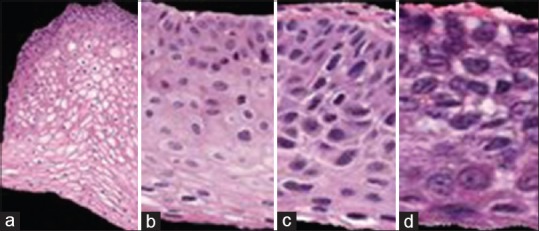
Cervical intraepithelial neoplasia grade label examples highlighting the increase of immature atypical cells from epithelium bottom to top with increasing cervical intraepithelial neoplasia severity. (a) Normal, (b) cervical intraepithelial neoplasia 1, (c) cervical intraepithelial neoplasia 2, (d) cervical intraepithelial neoplasia 3

As CIN increases in severity, the epithelium has been observed to show delayed maturation with an increase in immature atypical cells from bottom to the top of the epithelium.[1] As shown in Figure 1, atypical immature cells are seen mostly in the bottom third of the epithelium for CIN1 [Figure 1b]. For CIN2, the atypical immature cells typically appear in the bottom two-thirds of the epithelium [Figure 1c], and for CIN3, atypical immature cells typically are found in the full thickness of the epithelium [Figure 1d]. In addition to analyzing the progressively increasing quantity of atypical cells from bottom to top of the epithelium, identification of nuclear atypia is also significant.[1] Nuclear atypia are characterized by nuclei of abnormal shapes and sizes within the epithelium region. Visual assessment of this nuclear atypia may be difficult, due to a large number of nuclei present and tissue heterogeneity. This may contribute to diagnostic inter- and intra-pathologist variation.

Computer-assisted methods (digital pathology) have been explored for CIN diagnosis in other studies and provided the foundation for the work reported.[2] In depth literature reviews for related studies have been presented.[3,4] In addition, this paper builds off techniques for semi-automated CIN assessment for epithelium regions in digitized pathology images examining texture features, nuclei determination and Delaunay triangulation analysis,[5,6] medial axis determination, and localized CIN grade assessment. This paper extends the study,[3,4] for the development of image analysis and classification techniques for individual vertical segments obtained from partitioning the epithelium along the medial axis. A logistic regression classifier is explored for CIN classification for comparison with support vector machine (SVM) and linear discriminant analysis (LDA) classifier approaches for individual vertical segment classification. CIN grades from two pathologists for 118 digitized histology images are used as ground truth for CIN classification accuracy.

The order of the remaining sections of the article is as follows: Section II presents the image analysis and classification approaches used in this research; Section III describes the experiments performed; Section IV presents and analyzes the results obtained and a discussion; Section V provides the study conclusions.

METHODS

Figure 2 presents an overview of the approach for analyzing the digitized pathology epithelium images:

Figure 2.

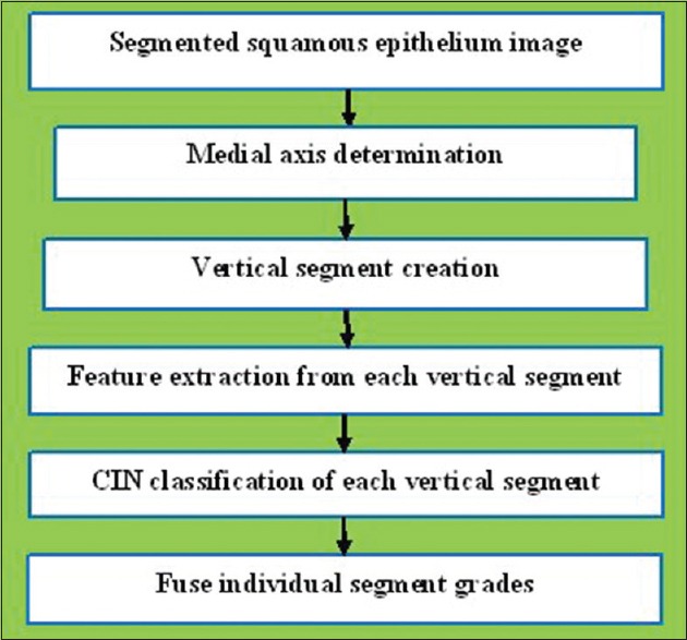
Digitized pathology epithelium image analysis procedures

• Step 1: Detect the medial axis of the segmented epithelium region

• Step 2: Divide the segmented image into 10 vertical segments orthogonal to the medial axis

• Step 3: Extract features from each of the vertical segments

• Step 4: Use the classification algorithms to classify each segment into one of the CIN grades

• Step 5: Fuse the CIN grades from every ten vertical segments in one image to obtain the CIN grade of the whole epithelium.

This approach was used in previous studies.[3,4] The following sections present each step in detail.

Pathologist Ground Truth Description

For the image and CIN classification techniques explored in this research, 118 full-color digitized histology images are used with H and E stain preparations of tissue sections of normal cervical tissue and three grades of cervical carcinoma in situ. This data set extends the 61 images used in previous studies.[3,4] In this study, expert pathologists (RZ, SF) provided CIN grades for the whole epithelium image and for the 10 vertical segments into which each image was partitioned [Figure 3 and Table 1].

Figure 3.

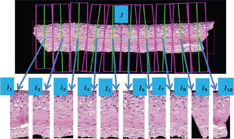
Epithelium image example with vertical segment images (I₁, I₂, I₂,…. I₁₀) determined from bounding boxes after dividing the medial axis into ten line segment approximations after medial axis computation

Table 1.

Ground truth cervical intraepithelial neoplasia grade labels for both experts

Note that, the CIN grades from the expert pathologists for the individual vertical segments within an image sometimes vary between the experts and that the CIN grades for the individual vertical segments can be different from the whole image. The ground truth is given as two groups of CIN grades for everyone segment out of our 118-image data set. Each single label is specified as a class number to denote the dysplasia and severe dysplasia. In this case, the pathologists gave “1” as Normal, “2” as CIN1, “3” as CIN2 and “4”, as CIN3. A pathologist labeled a vertical segment “0” if the pathologist was not able to make any CIN grade decision due to insufficient image information or detail (the 9^th segment in image 2 [RZ] and the 9^th and 10^th segment in image 4 [SF] [Table 1]). Since 118 digitized histology images are used in this study to create vertical segments for feature extraction and classification, 1180 segments in total are labeled by both pathologists to generate two groups of ground truth, respectively. Table 1 provides CIN labels from both pathologists (RZ/SF) for the 10 vertical segments from 10 histology images as examples of the experimental data set.

Table 1 shows that the two pathologists agree with each other on some of the segments and disagree on others. For example, from image 8, RZ assigns every segment as CIN3 (4), but SF only labels the 3^rd, 4^th, 6^th, and the 9^th as CIN3 (4) with the others as CIN2 (3). Part of the rationale for this paper is to show that the classification results for the individual vertical segments and the whole image are within the variation of the expert pathologist designations and that there is inter-pathologist variation within an image and for the image-based classification. [Table 1].

Three methods were used for assigning “truth labels” to the individual vertical segments, including the “0” labeled segments that the pathologists did not label, producing three (slightly) different sets of ground truth labels for evaluating the classification algorithms developed. The three methods examined to determine ground truth labels are:

1. Use the image label for every single segmentation regardless of the individual labels, which are denoted as “Image Label”

2. Keep the pathologist labels for the non-"0" segments and replace the “0” segments with the majority of individual labels by the pathologist within these 10 segments, which are denoted as “Major Sub”

3. Keep the pathologist labels for the non-"0" segments and replace the “0” segments with the whole image label by the pathologist, which are denoted as “Image Sub.”

Medial Axis Detection and Segments Creation

The method for computing the medial axis, which is based on the distance transform, is presented in detail.[4] The resulting medial axis is partitioned into ten segments of approximately equal length, perpendicular line slopes are estimated at the mid-points of each segment, and vertical lines are projected at the end points of each segment to generate ten vertical segments for analysis. The epithelium image is partitioned into ten vertical segments to facilitate localized diagnostic classification on sub-regions within the epithelium.

Feature Extraction

Features are computed for each of the ten vertical segments of the whole image, I₁, I₂, I₃,…. I₁₀. All the segments of one whole image are feature-extracted in a sequence, from left to right, I₁–I₁₀ [Figure 3]. These features were developed in previous research.[4] A summary of those features is presented here. In total, five different types of features were computed, including: (1) Texture features (F1–F10),[3] (2) cellularity features (F11–F13), (3) nuclear features (F14, F15), (4) acellular (light area) features (F16–F22), (4) combination features (F23, F24), and (5) advanced layer-by-layer triangle features (F25–F27).[4]

Texture and color features

The texture and color features were used in our previous work and are described.[4] The texture features include contrast (F1), energy (F2), correlation (F3), and homogeneity (F4) of the segmented region, combined with the same statistics (contrast, energy, and correlation) generated from the gray level co-occurrence matrix (GLCM) of the segment (F5–F10). These features are generated using the statistics of the GLCM matrix[4,7,8] to describe the contrast and the uniformity of the region.

Nuclear features

The dark shading color feature discussed in the previous research[4] corresponds to nuclei, which appear within epithelial cells in various shapes and sizes. Nuclei tend to increase in both number and size as the CIN level increases.[1] This linkage between nuclear characteristics and CIN levels motivates our development of algorithms for nuclei detection feature extraction. In this research, the algorithms of nuclei detection and nuclear feature extraction are developed to obtain features to facilitate CIN classification. Specifically, the following steps are performed [Figure 5]:

Figure 5.

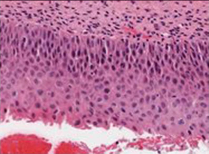
Misclassification example of a cervical intraepithelial neoplasia 2 image labeled as a cervical intraepithelial neoplasia 3

• Step 1: Cluster the histogram-equalized image into clusters of background (darkest), nuclei and lighter (lightest) epithelium regions using the K-means algorithm (K = 4). Generate a mask image containing the pixels closest to the nuclei cluster (second darkest)

• Step 2: Use the Matlab function imclose with a circular structuring element of radius 4 to perform morphological closing on the nuclei mask image

• Step 3: Fill the holes in the image from Step 2 with Matlab's imfill function for this process

• Step 4: Use the Matlab's imopen to perform morphological opening with a circular structuring element of radius 4 on the image from Step 3

• Step 5: Eliminate small area noise objects (nonnuclei objects) within the epithelium region of interest from the mask in Step 4, with the area opening operation using the Matlab function bwareaopen.

Acellular features

Extracting the light area regions is challenging due to the color and intensity variations in the epithelium images. Each of the L*, a*, and b* planes of CIELAB color space were evaluated for characterizing the light areas. It was empirically determined that L* provides the best visual results. The following outlines the methods used to segment the histology images:

• Step 1: Convert the original image from RGB color space to L* a* b* color space, then select the luminance component L* [Figure 4a]

• Step 2: Perform adaptive histogram equalization on the image from Step 1 using Matlab's adapthisteq. Adapthisteq operates on small regions (tiles)[2] for contrast enhancement so that the histogram of the output region matches a specified histogram and combines neighboring tiles using bilinear interpolation to eliminate artificially induced boundaries [Figure 4b]

• Step 3: After the image has been contrast-adjusted, the image is binarized by applying an empirically determined threshold of 0.6. This step is intended to eliminate the dark nuclear regions and to retain the lighter nuclei and epithelium along with the light areas [Figure 4c]

• Step 4: Segment the light areas using the K-means algorithm based on,[3,9] with K = 4. The K-means algorithm input is the histogram-equalized image from Step 2 multiplied by the binary thresholded image from Step 3. A light area clustering example is given in Figure 4d.

• Step 5: Remove from the image all objects having an area <100 pixels, determined empirically, using the Matlab function regionprops.[2] A morphological closing is performed with a disk structure element of radius 2. An example result is shown in Figure 4e.

Figure 4.

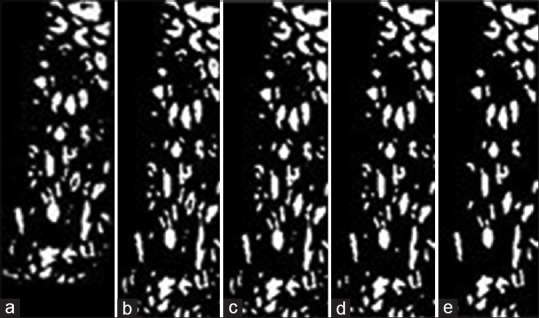
Image examples of nuclei detection algorithm. (a) Image with preliminary nuclei objects obtained from clustering (Step 1). (b) Image closing to connect nuclei objects (Step 2). (c) Image with hole filling to produce nuclei objects (Step 3). (d) Image opening to separate nuclei objects (Step 4). (e) Image with nonnuclei (small) objects eliminated (Step 5)

Combination features

After both the nuclear features and the acellular features were extracted, combination features were calculated with the intent to capture the relative increase in nuclei numbers as CIN grade increases. One is the ratio of the acellular number to the nuclei number (F23), and the other is the ratio of the acellular area to the total nuclei area (F24).

Triangle features

In this research, the Delaunay triangle method was used, but restrict the geometrical regions it can act upon, as follows. Before forming the Delaunay triangles,[5,10] with the vertices provided by the nuclei detection results from nuclear feature section, the vertical segment being processed is sub-divided into three vertical layers, as illustrated in Figure 6. The aim is to associate the presence of increasing nuclei throughout the epithelium with increasing CIN grades, namely: abnormality of the bottom third of the epithelium roughly corresponds to CIN1; abnormality of the bottom two-thirds, to CIN2; and abnormality of all three layers, to CIN3. These layers are referred to as the bottom, mid, and top.

Figure 6.

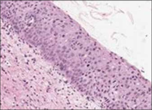
Misclassification example of a cervical intraepithelial neoplasia 2 image labeled as a cervical intraepithelial neoplasia 1

EXPERIMENTS PERFORMED

Experiments were performed using the data set consisting of 118 digitized histology images, which were CIN labeled by two experts (RZ and SF) (RZ: 38 normal, 26 CIN1, 26 CIN2, and 26 CIN3; SF: 40 normal, 25 CIN1, 24 CIN2, and 29 CIN3).

Fusion-based Cervical Intraepithelial Neoplasia Grade Classification of Vertical Segment Images

Labeling

The experimental data set consists of 118 digitized histology images with vertical segments obtained using the medial axis detection and vertical segment partitioning algorithms presented in Section IIB. An additional image from previous research[4] was used for image processing parameter determination. For this experimental data set, CIN grades were obtained for the 10 vertical segments from each image from both pathologists (RZ/SF), and the image analysis, feature extraction and classification approaches presented in Section II were performed for each vertical segment image. Epithelium image truth labels from both pathologists (SF and RZ) are used as a training and testing labels, unlike our previous study[4] where only one expert's truth label was used in training and testing. As described in Section IIA, the pathologists were unable to assign labels for some segments, for which the Image Label, Major Sub, and Image Sub methods were used to generate “truth labels” for these segments (Section IIA for definitions).

Classification

For CIN discrimination, all the features extracted from the vertical segment images were used as inputs to SVM, LDA, logistic regression, and random forest classifiers. The LIBSVM[11] implementation of the SVM and LDA classifiers were used, as in our previous study.[4] The SVM implementation uses a linear kernel with four weights as the fractions of the images in each CIN class (normal, CIN1, CIN2, and CIN3). Logistic regression had a multinomial logistic regression (MLR) model for predicting probabilities for each class.[12] Random forest,[13,14] used combinations of tree predictors such that each tree depends on the values of a random vector sampled with the same distribution for all trees in the forest.[14,15]

Individual features were normalized by subtracting the mean training set feature value and dividing by the standard deviation training set feature value.[4] In this approach, the classifier is trained based on the individual segment feature vectors for all but the left-out epithelium image (test image), which was called “leave-one-out” approach.[4] Four approaches were explored for using the CIN expert truth labels for the individual vertical segments and the whole epithelium image for classifier algorithm training and testing, including:

1. SF-SF CIN labels as training-testing labels

2. RZ-RZ CIN labels as training-testing labels

3. RZ-SF CIN labels for training-testing sets

4. SF-RZ CIN labels for training-testing sets.

Using the different pathologist CIN label training and test combinations for vertical segment classification, the influence on inter- and intra-pathologist CIN truth labels was examined on individual vertical segment classification accuracy.

Then, the predicted CIN grades of the vertical segment images were fused to obtain the CIN grade of the entire test epithelium image [Figure 3]. The fusion of the CIN grades of the vertical segment images was completed using a voting scheme.[4] The CIN grade of the test image was assigned to the most frequently occurring class over the ten vertical segments. If a tie was found among the most frequently appearing case of CIN grades, the test image was assigned with the higher/highest one (i.e., the most severe diagnostic grade). For example, if there was a tie between CIN2 and CIN3, then the image was assigned CIN3. As previously explained in Section IIA, there were four different ways of conducting our experiments by using different combinations of the labels from the two pathologists for training and testing. This resulted in four different groups of classification results. The input images for each group are the same 118 histological images.

Scoring schemes

Two scoring schemes were used for evaluating the results. Specifically, the same schemes were utilized as[4] for compatibility with those results. The schemes are summarized below:

Scheme 1 (exact class label): The first approach is exact classification, which means that a label was considered correct if and only if the class label assigned to the test image by our algorithm was the same as the ground truth label.

Scheme 2 (normal vs. CIN): For the second scoring scheme, the classification result was considered correct if and only if when a ground truth Normal grade was classified Normal by our algorithm and a ground truth CIN (1–3) grade was classified as CIN by our algorithm.

Feature Evaluation and Selection

In,[4] a SAS^® implementation of MLR[16,17,18,19,20] and a Weka^® attribute information gain evaluator were utilized for feature selection. MLR was used for modeling nominal outcome variables, and the P values obtained from the MLR output were utilized as criteria for selecting features when the P value is less than an appropriate alpha (α) value.[16,17,18,19] For Weka analysis, the features are ranked in an order by “attributes information gain ratio” where the higher the ratio, the more significant the feature will be.[4] Both feature evaluation methods are applied in this study to improve the classification outcomes as well as to keep the classification results comparable to the study by Guo et al.[4] Feature selection was done based on the whole image labels of RZ applied to the individual vertical segments.

EXPERIMENTAL RESULTS AND ANALYSIS

Experimental Results

As explained in the previous section, the vertical segment image classifications (CIN grading) were obtained using SVM, LDA, logistic, and random forest classifiers with a leave-one-image-out approach based on all the twenty-seven features generated for each vertical segment. This yields classification labels for each of the 10 vertical segments in an epithelium image. Then, the CIN classification for the whole epithelium image is obtained by fusing the vertical segment labels using a voting scheme. The performance of these epithelium image classifications was evaluated using the two scoring schemes presented in Section IIIA 3.

For the first set of experiments, individual vertical segment classification is examined. Each individual vertical segment is assigned a CIN grade label using the Image Label, Major Sub, and Image Sub approaches from Section IIA for training and testing the SVM, LDA, logistic regression, and random forest classifiers. For these experiments, individual vertical segment and whole image CIN labels are from the same expert for classifier training and testing, denoted as RZ-RZ and SF-SF for the two experts, respectively. Individual vertical segment exact class classification results are given in Table 2. From Table 2, the highest individual classification accuracy (81.29%/80.10% based on labels from RZ-RZ/SF-SF, respectively) for exact classification was obtained using the Logistic classifier based on the Image Label approach for assigning CIN class labels to the individual vertical segments (all vertical segments within an image are assigned the image CIN label). Accuracies of 62.71%/64.92% (RZ-RZ/SF-SF) and 60.16%/63.23% (RZ-RZ/SF-SF) were obtained using the SVM and LDA classifiers, respectively, based on the Image Label approach for individual vertical segment labeling, which were used in (Note that “RZ-RZ” means that RZ's labels were used for both training and testing in the referenced experiment; likewise for SF).[4]

Table 2.

Individual vertical segment exact class label classification results based on all 27 features using same expert labels for training-testing sets (RZ-RZ and SF-SF)

The second set of experiments examined the impact of feature selection on CIN classification accuracy for the individual vertical segments. For feature evaluation and selection experiments, all 27 features extracted from the individual vertical segments with CIN truth labels from RZ were used as inputs to the SAS MLR algorithm as well as the feature selector in Weka^®. A value of α = 0.05 was used to determine statistical significance for the input features for the SAS MLR. The Weka^® feature selector ranks the features by an “attribute information gain ratio” (AIGR) which ranges from 0 to 1, with larger values indicating greater significance for the feature. The overall twenty-seven features with P values are presented in Table 3.

Table 3.

Features with corresponding P and attribute information gain ratio

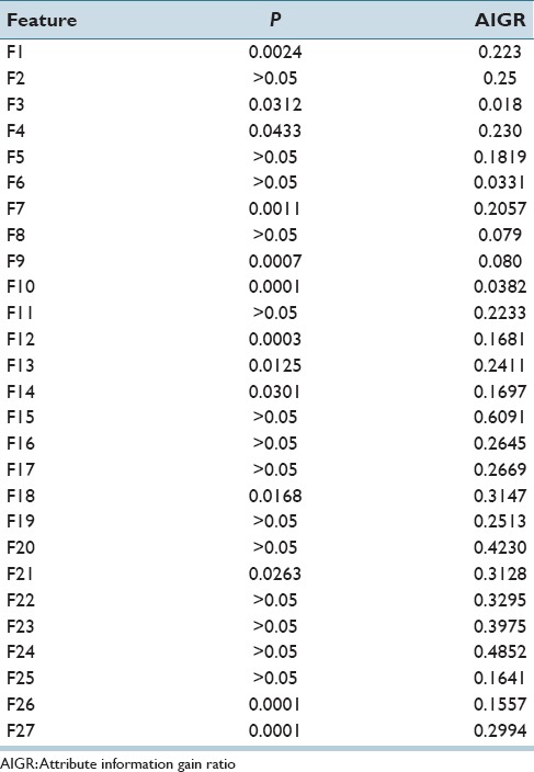
Based on the statistical significance of all the 27 features, the feature set selected using α = 0.05 consisted of F1, F3, F4, F7, F9, F10, F12, F13, F14, F18, F21, F22, F23, and F24. Note that all these features were selected based on the SAS MLR test of statistical significance except for F22, F23, and F24, which were selected since they have a relatively high information gain ratio (AIGR) among the 27 features [from 2^nd place to 4^th place in Table 3].[4] We compared discrimination accuracies using this reduced set of features to the results using the entire 27-feature set for fusion-based whole image classification based on (Section IIIA 2) for combining the individual vertical segment classifications. Individual vertical segment classifications were generated using the SVM, LDA, Logistic Regression, and Random Forest classifiers based on the Image Label, Major Sub, and Image Sub approaches for obtaining individual vertical segment CIN labels for classifier training. For these experiments, the training and testing CIN labels were from the same expert, denoted as RZ-RZ and SF-SF, respectively. Exact class label and normal versus CIN classification whole image results are reported for the different classifiers based on all 27 features in Table 4 and the reduced feature set in Table 5.

Table 4.

Fusion-based whole image percentage correct cervical intraepithelial neoplasia discrimination rates using all features using the same expert for training and testing sets

Table 5.

Fusion-based whole Image percentage correct cervical intraepithelial neoplasia discrimination rates using reduced features with the same expert for training and testing sets

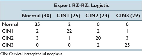
In Table 6, the best confusion matrix result obtained using RZ-RZ labels for training-testing for the reduced feature set is shown, with an exact class label classification of 88.98% and normal versus CIN classification of 94.92%. Our highest previous results[4] for a 61 image dataset were 88.5% (exact classification accuracy) and 95.1% (normal vs. CIN) using the LDA classifier and RZ-RZ training-testing labels. For comparison purposes, Table 7 presents the best confusion matrix result using RZ-RZ for training-testing for all 27 features on the 118 image set, which gives an exact class label classification of 86.44% and normal versus CIN classification of 94.92%.

Table 6.

Best confusion matrix results for fusion-based whole image classification using reduced feature set

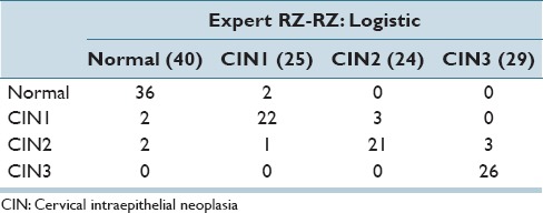
Table 7.

Best confusion matrix results for fusion-based whole image classification using all 27 features

Analysis of Results

In this section, we analyze the classification results from Section IVA, in four different ways: (a) a performance comparison among the classifiers (SVM, LDA, logistic, random forest) and (b) a performance comparison between previous research[4] and this study, (c) the impact on performance using intra- and inter-pathologist CIN truth labels for the classifier training and testing sets, and (d) a performance comparison between our classification results and the baseline results from the pathologists. The correct recognition rates for all classifiers investigated are presented using training-testing labels from RZ-SF/SF-RZ for all 27 features [Table 8] and the reduced feature set [Table 9].

Table 8.

Fusion-based whole image normal versus cervical intraepithelial neoplasia and exact cervical intraepithelial neoplasia discrimination rates using all 27 features (F1-F27) with expert training-testing labels of RZ-SF and SF-RZ

Table 9.

Fusion-based whole image normal versus cervical intraepithelial neoplasia and exact cervical intraepithelial neoplasia discrimination rates using reduced features with training-testing labels of RZ-SF and SF-RZ

From Tables 5 and 9, the logistic classifier exact class experiments for corresponding truth labels (Image Label, Image Sub, Major Sub) when reduced features are employed as the input feature vectors. The logistic classifier yielded a maximum improvement of 13.56% (75.42% from SVM and LDA to 88.98% for RZ-RZ) when using the truth tables from a single pathologist and a maximum improvement of 10.76% (71.95% from SVM to 82.71% for RZ-SF) using inter-pathologist truth tables as training and testing labels. In addressing with the unknown segments labeled as “0” by the pathologists, the labeling methods of Image Label and Major Sub had an impact on the overall classification results; the classification accuracies are improved when using the same classifiers but different labeling methods than the ones in previous research.[4]

From the classification results for individual segment classification presented in Table 2 of Section IVA, the logistic classifier gave an improvement of 10.19% (71.10% from LDA to 81.29% for RZ-RZ) and 8.49% (71.61% from LDA to 80.10% for SF-SF). Among all the results generated by the classifiers in this study, the highest individual segment classification accuracy is obtained with the logistic classifier, with the correct recognition rate of 81.29%. Compared with the accuracy obtained by the classifiers used in the previous research[4] SVM/LDA, the highest accuracy for the individual segment classification is 71.61%. An improvement of 9.32% is obtained by using logistic classifier. For fusion-based whole image classification using the complete feature set (27 features), shown in Table 4 of Section IVA, a decrease of 0.44% (88.5% LDA[4] to 86.44% logistic in this study) is obtained as the exact class image classification accuracy. A decrease of 2.6% (from 96.7%[4] LDA to 94.10% logistic in this study) is obtained as normal versus CIN correct rate. For the epithelium classification results using the reduced feature set shown in Table 5, a minimum improvement of 3.73% (from 85.25%[4] for LDA classifier to 88.98% in this study) is found. It can be observed that some of the classification accuracies drop when using one expert label as training and the other one as testing, compared with the results in Tables 8 and 9. For the logistic classifier, the highest exact classification rate was 88.98% [105/118 in Table 5] which was higher than 82.71% using one expert's labels for training (RZ) and the second expert's labels (SF) for testing [Table 9].

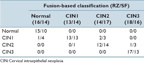
In examining the performance of our classification results, we also use the pathologists’ truth labels of epithelium images to generate a baseline for exact classification accuracy. As shown in Table 10, the confusion matrix is obtained by fusing the pathologist truth labels of individual labels with the same fusion techniques of voting scheme which has already been explained in Section II2. Note that for the individual vertical segment labels fusion; only the 61 images dataset is utilized to remain the study consistent with the previous study.[4] Table 10 highlights the variation in CIN grading for the expert pathologists for a 61 image data set, which differs from the 118 digitized histology image set used in this study. From Table 10, the experts RZ and SF had an exact class agreement in 78.7% (48/61) of the epithelium images. The experts differed by one CIN grade on the remaining 13 images (off-by-one). The exact class label fusion-based CIN discrimination results obtained in this study are comparable to the 78.7% expert agreement rate. The exact class LDA classifier result of 76.02% from Table 4 based on the training-testing CIN labels from RZ (denoted in this study as RZ-RZ) is based on the benchmark approach from the study by Guo et al.,[4] where 88.5% is the exact class correct classification rate based on a 61 image data set from the study by Guo et al.[4] It should be noted that the 118 digitized histology image set used in this research is a different data set than the 61 images from.[4] Consequently, the exact class discrimination rate of 76.02% provides the benchmark for comparing results in this study. The logistic regression classifier for the 118 image set yielded exact class discrimination results as high as 88.98%/85.51% (RZ-RZ/SF-SF) using the same expert for training-testing CIN labels and the image CIN label for each individual vertical segment, a 12.96%/5.94% (RZ-RZ/SF-SF) improvement for single expert over the baseline method.[4] The logistic regression method gave the highest vertical segment classification rate of 81.29%/80.10% (RZ-RZ/SF-SF), which fueled the higher fusion-based image classification. Overall, the CIN classification rates tended to be higher using the training-testing labels for the same expert than for training labels from one expert and testing labels from the other expert. Based on the logistic classifier, the same expert exact label results were 88.98%/85.51% (RZ-RZ/SF-SF) compared to training labels from one expert and testing labels from the other expert 82.71%/78.39% (RZ-SF/SF-RZ), an increase of 6.27%/7.12%, respectively. This result can be used to highlight the impact of building larger data sets where different experts are involved in truthing or diagnostically assessing parts of the data set.

Table 10.

Confusion matrix classification baseline obtained from pathologist ground truth labels

For the logistic and random forest classifiers, which performed better in this study, it appears that using the same CIN label for each vertical segment in training and testing the different classifiers compared to using the local, individual expert determined CIN labels for training and testing the different classifiers resulted in slightly higher overall exact label discrimination rates; there does not appear to be a corresponding trend in the exact label classification rates for the SVM and LDA classifiers. Guo et al.[4] reported the image-based exact label discrimination rates were much lower than the fusion-based voting of the individual vertical segment exact label classifications. It appears that the local CIN information from the individual vertical segments contributes to enhanced image-based exact label discrimination. However, variations in the vertical segment CIN truthing for an image do not appear to provide an improvement to an overall image CIN assessment.

The confusion matrix classification results presented in Table 9 show that by fusing the pathologists’ labels without any prediction from classifiers, RZ's labels give an exact classification accuracy of 93.44% (57/61) and SF's labels indicates an exact correct recognition rate of 81.97% (50/61). Moreover, from the exact classification accuracy, we obtained in this study, the highest result of 88.98% falls in the range of this baseline provided from those two pathologists.

Table 11 presents a summary of the highest CIN classification results determined from this study for the different classifiers and training-testing expert truth label combinations and the highest classification results obtained from the experiments performed.[4] From Table 11, the exact class label results for the 118 image set examined in this study are comparable to the results reported for the 61 image set[4] based on all 27 features and the reduced feature set. Individual vertical segment results were not reported.[4] However, applying the same LDA classifier[4] to individual vertical segment classification from the 118 image set in this study showed an improvement of 16.87% (from LDA classifier 60.16%/63.23% (RZ-RZ/SF-SF)) to logistic regression 81.29%/80.10% from [Table 2]). In addition, comparing the LDA approach from[4] for fusion-based image classifier for the 118 image set yielded an improvement of 13.56%/10.17% with the logistic regression classifier (from LDA classifier 75.42%/74.58% [RZ-RZ/SF-SF] to logistic regression 88.98%/84.75% from [Table 5]) using the reduced feature set, and an improvement of 12.96/5.94% (from LDA classifier 76.02%/79.57% [RZ-RZ/SF-SF]) to logistic regression 88.98%/85.51% from [Table 4]) using all 27 features. Since exact class label is the most stringent of the scoring schemes we used, we interpret these results as showing a substantial gain in classification accuracy when using the logistic regression classifier for the extended image dataset of 118 histological images over the approaches explored in previous research.[4]

Table 11.

Summary of best classification accuracies: Current study versus previous research versus current

For the logistic and random forest classifiers, which performed better in this study, it appears that using the same CIN label for each vertical segment in training and testing the different classifiers compared to using the local, individual expert determined CIN labels for training and testing the different classifiers resulted in slightly higher overall exact label discrimination rates; there does not appear to be a corresponding trend in the exact label classification rates for the SVM and LDA classifiers. This trend is observed in Table 11 where the majority of the highest classification results found in this study were based on the Image Label approach for individual vertical segment labeling for classifier training and testing. From,[4] the image-based exact label discrimination rates were much lower than the fusion-based voting of the individual vertical segment exact label classifications. It appears that the local CIN information from the individual vertical segments contributes to enhanced image-based exact label discrimination. However, variations in the vertical segment CIN truthing for an image do not appear to provide improvement to an overall image CIN assessment.

In examining the classification results, the majority of the exact class label classification errors are off-by-one CIN grade. Figure 5 shows an example of an image with expert label of CIN2 (RZ) that was labeled as a CIN3 by the LDA classifier.

From the basal membrane near the top of the epithelium in Figure 5 across the epithelium (downward toward the bottom), the nuclei distribution is relatively uniform in certain regions. The nuclear features, as well as the layer-by-layer Delaunay triangle features, highlight the relatively uniform distribution of nuclei in the vertical segments containing those regions, which correspond to a higher CIN grade. In other regions of the epithelium, the nuclei density is not as uniform across the epithelium, which could provide for a less severe CIN grade label for the epithelium.

Figure 6 shows an example of an image with pathologist label of CIN2 (RZ) that was labeled as a CIN1 by the logistic classifier. This image has the texture and nuclei distribution which is more consistent with a CIN2 grade. However, the relative small nuclei area and lower color luminance in the epithelium leads to a lower CIN grade misclassification.

The overall algorithm was found to be robust in successful identification of nuclei. To evaluate nuclei detection, we manually counted nuclei in the two lightest-stained slides and the two darkest-stained slides. An average of 89.2% of the total number of nuclei in all four slides was detected. The 89.2% nuclei detection rate observed represents an advance over the results of Veta et al.,[21] who detected nuclei at rates of 85.5%–87.5% (not strictly comparable, as these results were for breast cancer). The finding of a high percentage of nuclei in the lightest- and darkest-stained slides suggests that the algorithm is adaptable and robust with regard to varying staining.

The approach in this study expands the techniques of other studies that focus on the nucleus. We show in this work that the transition from normal to CIN3 affects the whole cell. We have shown that not only nuclei, but features of intercellular spaces are changed due to the more rapidly growing cells. Thus, one of the top four features by P value is the proportion of regions of cytoplasm in the image (F12).

CONCLUSION

In this study, we extended a localized, fusion-based image analysis approach for CIN classification to 118 digitized histology images. Twenty-seven features were explored, including the layer-by-layer triangle features and the nuclei as well as acellular features, as developed in previous research.[4] We conducted CIN discrimination experiments based on CIN truthing of the 118 image set by two pathologists (RZ/SF), including: (1) SF's CIN labels as training labels and testing labels. (2) RZ's CIN labels as training labels and testing labels. (3) RZ's CIN labels as training labels and SF's labels as testing labels. (4) SF's CIN labels as training labels and RZ's labels as testing labels. The vertical segments were classified using logistic regression, SVM, or LDA classifier, based on one of the four ways of labeled training data mentioned with a leave-one-out approach. We used a voting scheme to fuse the vertical segment classifications into a classification of the whole epithelium image. We evaluated the classification results with three scoring schemes, and compared the classification differences by classifiers, by scoring schemes, and the classification results of this research as compared to our previous work.[4]

Experimental results showed that the logistic and random tree classifiers outperformed the benchmark SVM and LDA classifiers.[4] The logistic regression classifier gave exact class discrimination results as high as 88.98%/85.51% (RZ/SF) using the same expert for training-testing CIN labels and the image CIN label for each individual vertical segment, which is a 13.56%/10.17% (RZ-RZ/SF-SF) improvement for single expert over the baseline method[4] using the reduced features. The CIN classification rates tended to be higher using the training-testing labels for the same expert than for training labels from one expert and testing labels from the other expert. The exact class label fusion-based CIN discrimination results obtained in this study are comparable to the exact class expert agreement rate.

Financial Support and Sponsorship

This research was supported (in part) by the Intramural Research Program of the National Institutes of Health, National Library of Medicine, and Lister Hill National Center for Biomedical Communications.

Conflicts of Interest

There are no conflicts of interest.

REFERENCES

- 1.Egner JR. AJCC cancer staging manual. J Am Med Assoc. 2010;304:1726. [Google Scholar]
- 2.Guo P. Cervical cancer histology image feature extraction and classification. Rolla, Missouri: Missouri University of Science and Technology; 2014. [Google Scholar]
- 3.De S, Stanley RJ, Lu C, Long R, Antani S, Thoma G, et al. A fusion-based approach for uterine cervical cancer histology image classification. Comput Med Imaging Graph. 2013;37:475–87. doi: 10.1016/j.compmedimag.2013.08.001. [DOI] [PMC free article] [PubMed] [Google Scholar]
- 4.Guo P, Banerjee K, Stanley R, Long R, Antani S, Thoma G, et al. Nuclei-based features for uterine cervical cancer histology image analysis with fusion-based classification. IEEE J Biomed Health Inform. 2015 doi: 10.1109/JBHI.2015.2483318. Doi: 10.1109/JBHI.2015.2483318. [DOI] [PMC free article] [PubMed] [Google Scholar]
- 5.Preparata FP, Shamos M. Computational Geometry: An Introduction. 3rd Ed. New York: Springer-Verlag; 1985. [Google Scholar]
- 6.He L, Long LR, Antani S, Thoma GR. Histology image analysis for carcinoma detection and grading. Comput Methods Programs Biomed. 2012;107:538–56. doi: 10.1016/j.cmpb.2011.12.007. [DOI] [PMC free article] [PubMed] [Google Scholar]
- 7.Gonzalez RC, Woods RE. Digital Image Processing. Vol. 2. Upper Saddle River, N.J: Prentice Hall; 2002. [Google Scholar]
- 8.Wang Y, Crookes D, Eldin OS, Wang S, Hamilton P, Diamond J. Assisted diagnosis of cervical intraepithelial neoplasia (CIN) IEEE J Sel Top Signal Process. 2009;3:112–21. [Google Scholar]
- 9.Mignotte M. Segmentation by fusion of histogram-based k-means clusters in different color spaces. IEEE Trans Image Process. 2008;17:780–7. doi: 10.1109/TIP.2008.920761. [DOI] [PubMed] [Google Scholar]
- 10.van der Marel J, Quint WG, Schiffman M, van de Sandt MM, Zuna RE, Dunn ST, et al. Molecular mapping of high-grade cervical intraepithelial neoplasia shows etiological dominance of HPV16. Int J Cancer. 2012;131:E946–53. doi: 10.1002/ijc.27532. [DOI] [PMC free article] [PubMed] [Google Scholar]
- 11.Chang C, Lin C. LIBSVM: A library for support vector machines. ACM Trans Intell Syst Technol. 2011;2:1–39. [Google Scholar]
- 12.Le Cessie S, Van Houwelingen JC Royal Statistical Society. Ridge estimators in logistic regression. J R Stat Soc Ser C Appl Stat. 1992;41:191–201. [Google Scholar]
- 13.Hall M, Frank E, Holmes G, Pfahringer B, Reutemann P, Witten IH. The WEKA data mining software. ACM SIGKDD Explor Newsl. 2009;11:10. [Google Scholar]
- 14.Breiman L. Manual on Setting Up, Using, and Understanding Random Forests v3. 1, Technical Report. Berkeley: Department of Statistics – University of California; 2002. [Last accessed on 2016 Nov 3]. p. 29. Available from: https://www.stat.berkeley.edu/~breiman/Using_random_forests_V3.1.pdf . [Google Scholar]
- 15.Breiman L, Cutler A. Breiman and Cutler's Random Forests for Classification and Regression. Package “randomForest,”. 2012. [Last accessed on 2016 Nov 3]. Available from: https://cran.r-project.org/web/packages/randomForest/randomForest.pdf .
- 16.Agresti A. An Introduction to Categorical Data Analysis. New York: John- Wiley & Sons, Inc; 2007. [Google Scholar]
- 17.Pal M. Multinomial logistic regression-based feature selection for hyperspectral data. Int J Appl Earth Obs Geoinf. 2012;14:214–20. [Google Scholar]
- 18.Li T, Zhu S, Ogihara M. Using discriminant analysis for multi-class classification: An experimental investigation. Knowl Inf Syst. 2006;10:453–72. [Google Scholar]
- 19.Hosmer DW, Lemeshow S. Applied Logistic Regression. 2nd ed. Hoboken, NJ: John Wiley & Sons; 1985. [Google Scholar]
- 20.Hall M, Frank E, Holmes G, Pfahringer B, Reutemann P, Witten IH. The WEKA data mining software: An update. ACM SIGKDD Explor. 2009;11:10–8. [Google Scholar]
- 21.Veta M, van Diest PJ, Kornegoor R, Huisman A, Viergever MA, Pluim JP. Automatic nuclei segmentation in H and E stained breast cancer histopathology images. PLoS One. 2013;8:e70221. doi: 10.1371/journal.pone.0070221. [DOI] [PMC free article] [PubMed] [Google Scholar]