How to interpret the results of medical time series data analysis: Classical statistical approaches versus dynamic Bayesian network modeling

Abstract

Background:

Classical statistics is a well-established approach in the analysis of medical data. While the medical community seems to be familiar with the concept of a statistical analysis and its interpretation, the Bayesian approach, argued by many of its proponents to be superior to the classical frequentist approach, is still not well-recognized in the analysis of medical data.

Aim:

The goal of this study is to encourage data analysts to use the Bayesian approach, such as modeling with graphical probabilistic networks, as an insightful alternative to classical statistical analysis of medical data.

Materials and Methods:

This paper offers a comparison of two approaches to analysis of medical time series data: (1) classical statistical approach, such as the Kaplan–Meier estimator and the Cox proportional hazards regression model, and (2) dynamic Bayesian network modeling. Our comparison is based on time series cervical cancer screening data collected at Magee-Womens Hospital, University of Pittsburgh Medical Center over 10 years.

Results:

The main outcomes of our comparison are cervical cancer risk assessments produced by the three approaches. However, our analysis discusses also several aspects of the comparison, such as modeling assumptions, model building, dealing with incomplete data, individualized risk assessment, results interpretation, and model validation.

Conclusion:

Our study shows that the Bayesian approach is (1) much more flexible in terms of modeling effort, and (2) it offers an individualized risk assessment, which is more cumbersome for classical statistical approaches.

INTRODUCTION

Classical statistics is the most often used approach in the analysis of medical data. The medical community seems to be most familiar with the concept of statistical modeling and its interpretation. Classical statistics has also become a common language for published medical data analyses. There are several approaches in statistics that allow one to analyze time series data. For example, life tables[1] express a lifetime risk, which is the number of patients who survive at each time interval instead of an actual point in time. Feuer et al.,[2] for example, applied a multiple decrement life table to calculate the lifetime risk of developing breast cancer. The Kaplan–Meier (KM) estimator[3] is another approach used in classical statistics to calculate risk expressed by a survival function estimated from time series data.[4,5] Cox proportional hazards regression (CPHR) model[6] allows for predicting the time at which an event of interest (e.g., death, disease recurrence) will occur. The method estimates the hazard ratio that expresses the impact of various explanatory variables on a response variable that represents the event of interest.[7,8,9,10]

One of the alternatives to classical statistical data analysis is based on subjectivist Bayesian view of probability. In this view, probability is a subjective measure of belief, rather than the limiting frequency in an infinite number of trials. An important practical consequence of adopting the Bayesian view of probability is that it allows for starting with an estimate of the probability that can be subsequently refined by observation. This opens up the possibility of applying sound statistical analysis to problems where data are scarce or missing altogether, and one has to start from a best guess estimate. A prominent tool used in Bayesian modeling is the Bayesian network[11] or its temporal version called dynamic Bayesian network (DBN).[12,13] While Bayesian networks have been used as modeling tools for almost three decades, their temporal extension, DBNs, found their way into medical modeling only in the last decade. There have been several practical applications of DBNs in medicine. For example, NasoNet, a system for diagnosis and prognosis of nasopharyngeal cancer,[14] or a DBN for the management of patients suffering from a carcinoid tumor.[15] DBNs have been also used in genomics and proteomics,[16,17] for example, in a prediction of protein secondary structure,[18] modeling peptide fragmentation[19] and cellular systems,[20] or in identifying gene regulatory networks from time course microarray data.[21,22,23] Other applications include reconstructing functional neuronal networks from spike train ensembles[24] or modeling dynamics of organ failure in patients in intensive care units.[25]

Despite the sizeable number of successful applications of DBNs, it seems that the medical community is still not too familiar with the Bayesian network approach. In this paper, we compare classical statistical approaches, such as the KM estimator and CPHR model to DBN modeling. Our comparison is based on the application of these approaches to the problem of cervical cancer screening. A subsequent aim of this paper is to encourage the medical community to consider other than classical statistical methods in data analysis. In our paper, we do not provide a detailed description of the approaches since it can be found in various textbooks and publications. We instead focus on the intuition behind each of the approaches.

The remainder of this paper is structured as follows. Section 2 describes methods and materials that we used in our study. Section 3 presents the results of our time series data analysis based on the classical statistical methods and DBN modeling. Section 4 discusses different aspects of the comparison. Finally, Section 5 summarizes our comparison study.

MATERIALS AND METHODS

We based our comparison study on a cervical cancer screening data set collected at the Magee-Womens Hospital (MWH), University of Pittsburgh Medical Center, Pittsburgh, USA. Screening for cervical cancer is a well-established practice that has dramatically reduced the incidence and mortality of this type of cancer.[26] Our data were collected over 10 years (from January 2005 to July 2015) and contain mainly the results of screening tests for cervical cancer. The primary screening test for cervical cancer in the USA is a cytology test called a PAP test (the term PAP comes from the last name of Dr. George Papanicolaou, who developed a cytology test), which is accompanied in some cases by a high-risk human papillomavirus (hrHPV) test (hrHPV test).

The MWH data contain 1,009,058 PAP test results belonging to 356,285 women. Around 29.4% of all PAP test results are accompanied by the hrHPV test results. Since we deal with a screening population, most of the patients in our data set are healthy women and only around 10% of the PAP test results are followed by a histopathological examination which is a diagnostic procedure. The data have been collected by means of advanced technologies, for example, cytology test interpretations were assisted with a computer-based system that identifies abnormal cells. The data contain also some clinical information such as a history of infections, cancer, use of contraceptives, or the human papillomavirus (HPV) vaccine status. To date, there are 2,864 patient cases with the HPV vaccine status recorded.

While building any model based on time series data, follow-up becomes a crucial issue. In our analysis, we excluded the vaginal PAP test results and those patients who had only one cytology test performed and did not have any follow-up data recorded. This led us to the analysis of 753,278 cytology test results belonging to 211,980 patients. Table 1 captures more information on the follow-up data.

Table 1.

The follow-up data

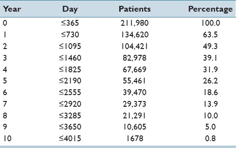
Year 0 indicates the year when a patient showed up for a screening or a diagnostic test for the first time. Of all patients who appeared in the database, 63.5% appeared for the follow-up screening in year 1, whereas 49.3% appeared for year 2, etc., Only 0.8% of all patients appeared in year 10 (this corresponds to 1,678 patients). In the reminder of this paper, we will indicate the beginning of a follow-up as t = 0. We will also apply two different time granularities: (1) a day granularity and (2) a year granularity. Table 1 contains the mapping of years to days.

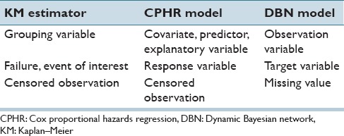
In our study, we have applied classical statistics approaches such as the KM estimator and CPHR, and the alternative method: DBN modeling. Because the approaches that we describe use different terminology, we included a mapping of various terms in Table 2. For example, the second row in Table 2 describes the terms used for the output variable, which is called depending on the approach: a failure, an event of interest, response, or a target. For the purpose of this paper, we will use the regression approach terminology, that is, we will refer either to a covariate or to a response variable.

Table 2.

Terminology mapping between the approaches

RESULTS

In this section, we present the results of the analysis that we have performed based on the MWH data. To analyze the cervical cancer screening data, we have selected those cases that have both screening test results available at t = 0 and that have at least one cytological or histological follow-up. There were 32,968 cases that met this requirement. In our analysis, we have included three covariates: PAP test, hrHPV test, and age with the values that were recorded at the beginning of the follow-up (t = 0) and a response variable representing the occurrence of precancer or invasive cervical cancer (CIN3+ includes the following diagnostic categories: precancer represented by cervical intraepithelial neoplasia Grade 3 (CIN3) and adenocarcinoma in situ (AIS), and invasive cervical cancer). We were interested in predicting the risk of CIN3+ over a period of 5 years. The two covariates were categorical: (1) the PAP test with the results: Negative, low-grade squamous intraepithelial lesion (LSIL), atypical squamous cells of undetermined significance (ASCUS), atypical glandular cells (AGC), atypical squamous cells - cannot exclude HSIL (ASC-H), high-grade squamous intraepithelial lesion (HSIL), suspicious or positive malignant cells (SUSP/POS); (the Pap test results follow the Bethesda classification) and (2) the hrHPV test with the results: positive and negative. The third covariate, age, was continuous with a mean value equal to 39.2 and a standard deviation equal to 13.3.

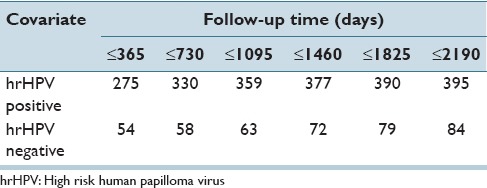
Table 3 presents the cumulative number of cases that developed CIN3+ for the two possible results of the hrHPV test: Positive and negative. There were 8,555 women with a positive hrHPV test result and 24,413 women with a negative hrHPV test result at the beginning of the follow-up. For example, we can see that in the period between 1,460 and 1,825 days of the follow-up, there were 13 new cases that developed CIN3+ (those cases had a positive hrHPV test result at t = 0). For a negative hrHPV test result, there were seven such cases during the same period.

Table 3.

Number of patients that developed CIN3+ (cumulative)

The Kaplan–Meier Estimator

The KM estimator is calculated based on the exact failure and censoring observations. For cervical cancer screening data, a failure, that is, an event of primary interest, is the presence of cervical precancer or cervical invasive cancer (CIN3+). Similarly to,[5] we have censored the patient data at the last registered testing date (cytological or histopathological) or at the time when they were diagnosed with CIN3+. The main outcome of the KM estimator is its survival function, which usually outlines the cumulative proportion of patients that survived. Since our analysis involved calculating a cumulative proportion of patients that developed the disease, instead of presenting a survival function, we will be plotting a 100% – survival function. This curve represents a cumulative proportion of patients that developed CIN3+ over 5 years.

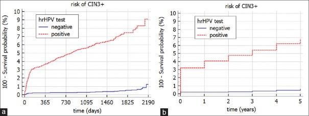
Figure 1 presents the KM curves for the patients that had both screening test results available at the beginning of the follow-up (t = 0). It compares two different groups depending on the hrHPV test result at the beginning of the follow-up (t = 0). These two groups correspond to two possible results of the hrHPV test: positive and negative and are statistically significantly different (log-rank test, P < 0.0001). Figure 1a shows that the risk of developing CIN3+ for the group of patients with positive hrHPV (t = 0) test result is 9.2% after 2,190 days, whereas a negative result of hrHPV (t = 0) is associated with a risk of 1.3% after 2,190 days. In addition, we have included the analysis of the same data with a time granularity represented by a year [Figure 1b]. Please, note that by changing the time granularity, the risk decreases and reaches 6.9% for women with a positive hrHPV (t = 0) test result and 0.6% for women with a negative hrHPV (t = 0) test result.

Figure 1.

The Kaplan–Meier curves for a risk of CIN3+ stratified by the high risk human papilloma virus test result (t = 0) with two time granularities (a) day, and (b) year

The Cox Proportional Hazards Regression Model

The CPHR model[6] is used in time series data analysis. It allows for: (1) predicting the time at which a response variable will occur and (2) investigating the effect of covariates on the response variable. The analysis is based on the hazard function that explains how the risk changes over time.

We have built the CPHR model for the cervical cancer screening using the same data that we used for the KM model. Table 4 presents the results of this analysis. It captures the effect of the covariates on the response variable representing a development of CIN3+. Each covariate is associated with a P value calculated based on the Wald test. The results show that there is a statistically significant contribution of each of the covariates to the response variable. Negative PAP test result and negative hrHPV test result are reference states in our analysis, and for the covariate representing age, a reference state is a mean value, which is in this case 39.2. Positive value of a regression coefficient β for a covariate indicates an increase of the risk of developing CIN3+ and a negative coefficient indicates a decrease of risk of developing CIN3+. The fifth column in Table 4 represents a hazard ratio exp(β) and it shows quantitatively the impact of each covariate on the response variable. For example, as age increases by 1 year, the risk of CIN3+ increases by 1% (exp(β) =1.01). The increase by 1 year refers to the mean age (i.e. 39.2 years). Similarly, for the hrHPV test, once the result goes from negative to positive, the risk increases by 675% (please note that exp (1.91) =6.75). With respect to the PAP test, once the result goes from negative to AGC result, the risk increases by 2913% (exp(3.37) =29.13).

Table 4.

Results of the Cox proportional hazards regression model

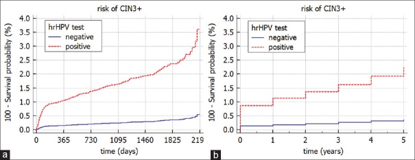
The CPHR model allows for generating also the survival curves. Figure 2 plots the survival curves for the two possible values of the hrHPV test and the mean value for other covariates in the model. We can see that the risk of developing CIN3+ depends on the initial result of the hrHPV test, that is, positive hrHPV test result at t = 0 leads to the risk of CIN3+ equal to 3.6% after 2190 days while negative hrHPV test result at t = 0 leads to the risk of CIN3+ equal to 0.6% after 2190 days. Please, note that by changing the time granularity the risk decreases and is equal to 2.3% for women with a positive hrHPV (t = 0) test result and 0.4% for women with a negative hrHPV (t = 0) test result [Figure 2b].

Figure 2.

The Cox proportional hazards regression model: Survival curves for the risk of CIN3+ stratified by the high risk human papilloma virus test result (t = 0) with two time granularities (a) day; (b) year

Dynamic Bayesian Network Modeling

Bayesian networks[11] are probabilistic graphical models that are capable of representing complex, uncertain knowledge. A Bayesian network is an acyclic directed graph modeling a structure of the domain and a joint probability distribution over its variables. This multivariate method allows for modeling a subjective expert knowledge as well as objective data. Reasoning algorithms for the Bayesian networks compute the posterior probability distribution over some variables of interest given a set of observations. DBN models are a temporal version of Bayesian networks and allow to model systems changing in time.

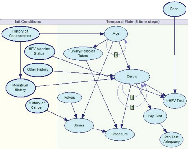
The Pittsburgh Cervical Cancer Screening Model (PCCSM)[27,28,29] is a DBN model for cervical cancer screening. The current version of the model consists of 15 variables. We based the structure of our model on textbook and expert knowledge and parametrized it by means of the MWH data. The graphical structure of the PCCSM model represents the existence of probabilistic relationships among the variables. We discretized the covariate age into three intervals: below 30, between 30 and 50, and 50 and up. This discretization was suggested by our expert, and it corresponds to three different cervical cancer risk groups. The time step that we have chosen in the PCCSM model was 1 year. This is a consequence of cervical cancer screening guidelines in U.S., recommending a woman to come for her PAP test examination once a year. Furthermore, for each patient in the data set we defined the initial time as t = 0, the year when the woman got registered in the MWH database, that is, when she showed up for the PAP test or a diagnostic test for the first time. The time horizon modeled in the PCCSM model was 5 years. The PCCSM generates a risk of developing CIN3+ over time. This risk is represented by the posterior probability distribution calculated by the model.

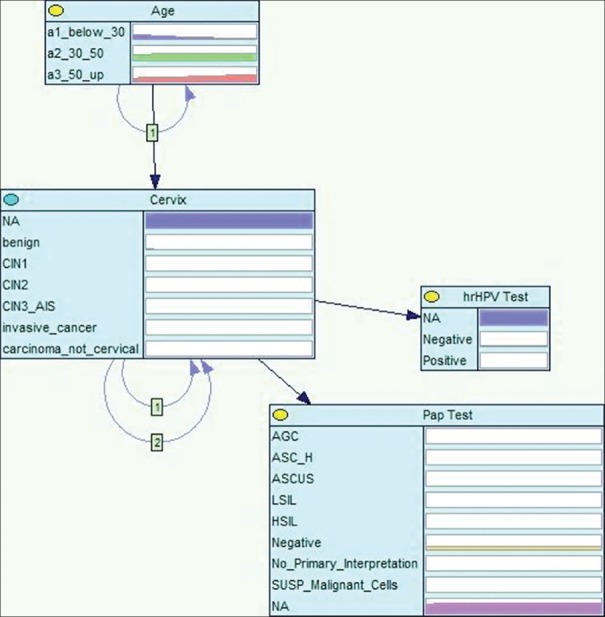
To perform a fair comparison, for the purpose of this paper, we have limited the PCCSM model to the covariates included in the KM and CPHR analyzes: that is, the PAP test, the hrHPV test, and age. The response variable is modeled in the PCCSM by the node cervix [Figure 3] and the covariates are modeled respectively by the following nodes: Pap test, hrHPV test, and age. The node cervix represents possible diagnoses including CIN3+. In reality, our model includes more covariates and is capable of considering other relevant factors and offering patient-specific results. Figure 4 shows a complete version of the PCCSM model consisting of 15 variables.[29]

Figure 3.

A highly simplified version of the Pittsburgh Cervical Cancer Screening Model

Figure 4.

A complete version of the Pittsburgh Cervical Cancer Screening Model

For each patient in the data set, we entered into the PCCSM model the evidence for the node representing the hrHPV test and then observed the posterior probability distributed over the node cervix over time. We were particularly interested in the posterior probability generated for the states CIN3/AIS (cervical precancer) and invasive cancer that represent CIN3+. Figure 5 captures the cumulative risk of CIN3+ over 5 years calculated by the PCCSM model. The risk is stratified by the results of the hrHPV (t = 0) test: positive or negative. Similarly to previous models, we can see that the risk of developing CIN3+ depends on the initial result of the hrHPV test, i.e., positive hrHPV test result at t = 0 leads to the risk of 3.9% after 5 years while negative hrHPV test result at t = 0 leads to the risk of 0.5% after 5 years. Similarly to the CPHR model, we also checked how the risk of CIN3+ is changing when PAP test result goes from negative to AGC result. The 5 years risk increases from 0.22% for a negative PAP test observed at t = 0 to the risk of CIN3+ equal to 4.2% for the PAP test with a result AGC at t = 0.

Figure 5.

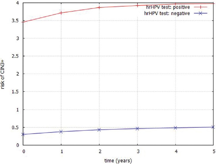
Cumulative risk of CIN3+ generated by a simplified Pittsburgh Cervical Cancer Screening Model stratified by the high risk human papilloma virus test result (t = 0)

DISCUSSION

In this section, we compare the two approaches used in time series data analysis, that is, the classical statistical approaches with the DBN modeling. We based our comparison on the following aspects: model assumptions, model building, dealing with incomplete data, individualized risk assessment, results interpretation, and model validation.

Assumptions

The KM estimator can be applied to data that represent nonrecurrent response variable. The CPHR model assumes that the effect of each of the covariates (risk relative to the baseline risk) is constant over time. DBN models assume to be stationary, that is, while the values of covariates change over time, the model itself does not. However, in general, the DBN models can be used to model nonstationary processes.[30] In CPHR model, a relationship between the response variable and the covariates should be linear. In DBNs, the relationships between the variables do not need to be necessarily linear. In the case of continuous variables, exact algorithms exist for multivariate Gaussian case (please note that this implies linear dependencies), whereas other cases can be dealt with by means of Monte Carlo methods, converting all distributions to a mixture of Gaussians or mixture of truncated exponentials or through dynamic discretization. Both the CPHR and the DBN models allow for including in the analysis mixtures of categorical and continuous variables. Our DBN model presented above is based on categorical variables, although the DBN approach, in general, is not limited to categorical variables and discrete probability distributions.

Model Building

Data are important in all three, although they are crucial in the classical statistical approaches. Building the KM estimator or the CPHR model is a data-driven process. If there are no data, the statistical analysis cannot be performed. Before building the KM estimator or the CPHR model, we have to prepare the data and identify patient cases that are censored. Subsequently, we estimate the survival function and calculate the regression coefficients for covariates. Building a DBN model does not, strictly speaking, require data, as the model can in the extreme, when no data are available, be based entirely on subjective estimates of probabilities. When data are available, they can potentially improve the model. Constructing a DBN model consists of two stages: (1) specification of the model structure and (2) elicitation of the numerical parameters. The structure of the model encodes typically causal relationships among the variables while the numerical parameters quantify these relationships. If there are no data available, expert opinion can be used to quantify the model. However, it is not an easy task, especially if the model requires thousands of probabilities to elicit. Both the structure and the numerical parameters of a DBN model can be also induced directly from the data by means of learning algorithms.[31,32]

The KM estimator, learned entirely from data, simply shows the relationship between two variables: the response variable and time. In addition, we can add a covariate that will group the data, and as a result, we will have a few survival functions corresponding to groups determined by a covariate. The CPHR model allows one to investigate the effect of several covariates on the response variable. The DBN modeling goes further, as it can model not only the relationships among covariates and the response variable, but it allows one to model interactions among all variables in the model. In addition, interactions can be immediate but can work over time including influences that span over several time steps.

The KM estimator and the CPHR model are flexible in terms of modeling time intervals, that is, we can choose different time granularity like day, month, or year. Theoretically, for a DBN model we could also choose a day as a possible transition interval between two slices, although in the presented application to cervical cancer screening it would be counter-productive to quantify the model with a day transition interval. First, there are no data available to assess numerical parameters since a screening test is usually performed annually. Second, modeling a time granularity as a day for the problem of cervical cancer screening seems to be unnecessary since a development of cervical cancer usually takes years.

Incomplete Data

The KM estimator and the CPHR analyzes can handle missing values in follow-up data. This incomplete information refers mainly to missing values for the response variable. Especially, it can handle right-censored data, that is, patient data that are lost from the follow-up before a response variable occurs. Censoring indicates removing the patient data from the calculations of the estimator at the end of their follow-up time. Censoring patient data decreases the sample size of patients at risk and by this, reduces the reliability of the KM estimator. If there are no censored cases in the data, then the KM curve will represent the true population distribution.

In case of a DBN model, there are two situations to consider in the context of possible missing values: (1) learning numerical parameters, and (2) reasoning with the model. DBNs can handle missing data naturally in both cases. Learning numerical parameters of a DBN model from incomplete data is facilitated by the expectation maximization algorithm,[33] which is designed to deal with missing observations. Reasoning with a DBN model does not require complete information on a patient to calculate risk for a response variable, that is, the posterior probability distributions is calculated only based on observed covariates that are not missing. This is different from the CPHR model, where every risk factor is assumed to be known and either present or absent.

Missing data for categorical variables in all three approaches can be treated as an additional state, although it can cause a problem if there is incomplete information for a continuous variable. In general, too many missing values may decrease the quality of the results. In case of the PCCSM model, the missing data were modeled as an additional state. Please, note that three nodes in Figure 3 have a state NA that stands for not available. This kind of modeling has a significance in some situations, for example, around 50% of all cervical cancer cases in our data did not have a screening history. Therefore, if there is no screening test result available, the model indicates increased risk of cervical cancer.

Results Interpretation

The output of the KM estimator is a survival function, often presented graphically as a survival curve. The survival function represents a cumulative proportion of patients that have survived. This approach is often used to compare survival curves for several patient groups. A CPHR model allows for analyzing the effect of several covariates on the response variable. The model calculates whether the covariate significantly influences the response variable. The method shows also quantitatively how the risk is changing depending on the value of a covariate. The results of this analysis can be also presented graphically by a survival curve. The output of a DBN model includes posterior probability distribution for the response variable over time given observed covariates. This approach is more flexible in calculating the results for various queries, i.e., a response variable can be easily changed and risk can be calculated for any model variable in question. Bayesian networks, furthermore, allow to calculate a diagnostic value for each covariate. In GeNIe software (BayesFusion LLC, Pittsburgh, USA), which we used in constructing our model, it is based on cross-entropy between each of the observed covariates and the response variable. Therefore, we can also quantify the effect of each covariate on the response variable.

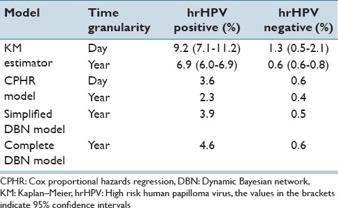
Table 5 shows the cumulative 5 years risk assessments for CIN3+ produced by the three approaches. For example, according to the KM estimator, women with a positive hrHPV test result at the beginning of the follow-up will have after 5 years a risk of 9.2%, whereas the CPHR model produces for the same patient group a risk of 3.6% of developing CIN3+ after 5 years. A simplified DBN model shows a risk of 3.9% after 5 years while a complete DBN model shows a risk of 4.6%. Please note, that for the statistical approaches we have included also the results for two-time granularities: (1) a day and (2) a year. It seems like the selection of a time granularity effects the final results produced by the KM estimator or the CPHR model. The results produced by these models with a year granularity are lower by 25%–50% while compared to the same models with a day granularity.

Table 5.

CIN3+risk assessments

Individualized risk assessment

The KM analysis focuses on the construction of a survival curve based on retrospective data rather than a classification of new cases. Theoretically, it is possible to prepare the data in such way that a patient in question will belong to the group of patients representing the survival function. In that case, for each patient, we would need to prepare a separate analysis. Thus, it may happen that there are too few patient cases in the data having the same set of observations as the patient in question for which we want to assess an individual risk.

Calculating individualized risk for a new patient based on a CPHR model consists of using the baseline cumulative hazard and then combining coefficients of various model covariates. However, combining the effect of different covariates is not straightforward, especially if a variable is continuous with a reference state equal to a mean value, which sometimes can be difficult to interpret.

The DBN approach allows for individualized management of patients and computes patient-specific risk based on observed covariates. Calculating an individualized risk for a new patient is pretty straightforward: All available patient information is entered into the model and the risk, expressed by the posterior probability, is instantly generated. It is important to note that not all information on a patient needs to be observed. Furthermore, we can calculate risk for different variables that are modeled. For example, in case of the PCCSM model, we can calculate the posterior probability for any variable in the model, not only for the response variable.

Stratification of risk categories

The KM estimator can calculate survival curves representing different groups of patients. Furthermore, these groups can be compared by means of a statistical test, which will show whether there is a statistically significant difference between the groups. Figure 1 shows two groups of patients categorized based on the hrHPV test result at the beginning of the follow-up, a log-rank test was used to verify whether the groups represent statistically significantly different risk of developing CIN3+. A CPHR model allows to calculate the survival functions for all categories of the covariate (if it is categorical) and for mean values for all other covariates in the model. The DBN modeling allows to look at risk assessments from different perspectives. For example, it allows to identify groups of patients that are at a higher or at a lower risk of developing CIN3+ given a set of values of covariates.

Model Validation

The regression models, such as the CPHR model can be validated externally.[34] External validation includes a comparison of models constructed from two independent data sets that are often called: (1) derivation data and (2) validation data. Unfortunately, most of the published Cox regression analyses do not include the results of such external validation. Mallett et al.[35] have analyzed 47 studies of which 44 were based on Cox regression model. The report shows that the assumption of proportional hazards was performed and presented only in around of 23% of the studies, while model validation was reported in around of 34% of the studies. There are also several measures such as-2 LogL, AIC, SBC, R² or likelihood ratio used in regression models. However, they express goodness of data fit to the model rather than its validation. Validation of DBN models is usually performed based on cross-validation techniques such as k-fold validation or its special case, the “leave-one-out” method.[36]

CONCLUSIONS

In this paper, we have compared two classes of approaches to time series data analysis in medicine: (1) the classical statistical approaches of the KM estimator and the CPHR model and (2) the DBN modeling. The two presented classical statistical approaches are well-established methodologies in medical data analysis, whereas DBN modeling is only starting to penetrate the field. We have compared these approaches along the following dimensions: assumptions, model building, dealing with incomplete data, individualized risk assessment and its interpretation, and model validation. In this comparison, we have used models based on the cervical cancer screening data collected at the MWH, University of Pittsburgh Medical Center, Pittsburgh, USA.

One of the limitations of the KM estimator is that it is based only on categorical variables. The other two approaches, that is, the CPHR and DBN models allow for including in the analysis both categorical and continuous variables.

Statistical approaches, like the KM estimator and the CPHR model, are fully dependent on data. If there are no data, the statistical analysis cannot be performed. The DBN modeling also rely on data. However, if data are not available, expert opinion can be used to build and quantify the model. Elicitation of numerical parameters for DBN from experts is not an easy task due to the number of probabilities that have to be acquired. There exist a variety of approaches to this problem, including standardized distributions and tools for semi-automatic estimation of probabilities.

The KM analysis is a method that estimates a survival function for a response variable, where time is considered the most important variable. Therefore, if there are any (other than time) significant covariates that influence the response variable, then the results of the KM analysis may be misleading and can obscure important differences between the groups of patients formed by these covariates. The CPHR and DBN approaches allow for multivariate analysis that models relationships among the variables. The CPHR analysis includes only modeling relationships between covariates and the response variable. The DBN modeling is more flexible, and it allows for modeling the relationships between any variables included in the analysis, that is, it can model not only the relationships among covariates and the response variable, but it can also capture the relationships among the covariates.

Our comparison shows that the DBN approach is more flexible in terms of an individualized risk assessment than the classical statistical approaches. The DBNs allow for looking at risk assessments from different perspectives and identify groups of patients that are at higher risk of developing a disease. Statistical approaches are quite well-established in the field while it seems that the Bayesian approach is still undervalued and only starting to penetrate the field. In the classical statistical approach, a final decision is based on the resulting P value, while in a Bayesian approach, such as the DBN modeling, a decision is made based on the posterior probability generated by the model. Because the result of a Bayesian analysis is the posterior probability distribution, individualized for a patient, it is straightforward to extend the analysis with a utility function and support the patient's decision using both the patient's current state and his or her preferences. It looks like medical community is much more familiar with the classical statistics, and they understand how to interpret the resulting P value. We have experienced in our practice that medical doctors typically expect the results of analysis to produce a P value and frame their analysis in terms of the difference between two posterior probabilities which are or are not statistically significant. This approach suffers from fundamental problems discussed by several authors.[37,38,39,40]

Financial Support and Sponsorship

Nil.

Conflicts of Interest

There are no conflicts of interest.

REFERENCES

- 1.Spiegelman M. The versatility of the life table. Am J Public Health Nations Health. 1957;47:297–304. doi: 10.2105/ajph.47.3.297. [DOI] [PMC free article] [PubMed] [Google Scholar]
- 2.Feuer EJ, Wun LM, Boring CC, Flanders WD, Timmel MJ, Tong T. The lifetime risk of developing breast cancer. J Natl Cancer Inst. 1993;85:892–7. doi: 10.1093/jnci/85.11.892. [DOI] [PubMed] [Google Scholar]
- 3.Kaplan EL, Meier P. Nonparametric estimation from incomplete observations. J Am Stat Assoc. 1958;53:457–81. [Google Scholar]
- 4.Castle PE, Sideri M, Jeronimo J, Solomon D, Schiffman M. Risk assessment to guide the prevention of cervical cancer. Am J Obstet Gynecol. 2007;197:356–e1-6. doi: 10.1016/j.ajog.2007.07.049. [DOI] [PMC free article] [PubMed] [Google Scholar]
- 5.Dillner J, Rebolj M, Birembaut P, Petry KU, Szarewski A, Munk C, et al. Long term predictive values of cytology and human papillomavirus testing in cervical cancer screening: Joint European cohort study. BMJ. 2008;337:A1754. doi: 10.1136/bmj.a1754. [DOI] [PMC free article] [PubMed] [Google Scholar]
- 6.Cox DR. Regression models and life tables. J R Stat Soc Ser B. 1972;34:187–220. [Google Scholar]
- 7.Gratwohl A, Hermans J, Goldman JM, Arcese W, Carreras E, Devergie A, et al. Risk assessment for patients with chronic myeloid leukaemia before allogeneic blood or marrow transplantation. Chronic leukemia working party of the European group for blood and marrow transplantation. Lancet. 1998;352:1087–92. doi: 10.1016/s0140-6736(98)03030-x. [DOI] [PubMed] [Google Scholar]
- 8.Liu J, Hong Y, D’Agostino RB, Sr, Wu Z, Wang W, Sun J, et al. Predictive value for the Chinese population of the Framingham CHD risk assessment tool compared with the Chinese multi-provincial cohort study. JAMA. 2004;291:2591–9. doi: 10.1001/jama.291.21.2591. [DOI] [PubMed] [Google Scholar]
- 9.Thompson I, Stephenson AJ, Scardino PT, Eastham JA, Bianco FJ, Jr, Dotan ZA, et al. Postoperative nomogram predicting the 10-year probability of prostate cancer recurrence after radical prostatectomy. J Clin Oncol. 2005;23:7005–12. doi: 10.1200/JCO.2005.01.867. [DOI] [PMC free article] [PubMed] [Google Scholar]
- 10.Moscicki AB, Ma Y, Wibbelsman C, Darragh TM, Powers A, Farhat S, et al. Rate of and risks for regression of cervical intraepithelial neoplasia 2 in adolescents and young women. Obstet Gynecol. 2010;116:1373–80. doi: 10.1097/AOG.0b013e3181fe777f. [DOI] [PMC free article] [PubMed] [Google Scholar]
- 11.Pearl J. Probabilistic Reasoning in Intelligent Systems: Networks of Plausible Inference. San Mateo, CA: Morgan Kaufmann Publishers, Inc; 1988. [Google Scholar]
- 12.Dean T, Kanazawa K. A model for reasoning about persistence and causation. Comput Intell. 1989;5:142–50. [Google Scholar]
- 13.Kjaerulff U. In: A computational scheme for reasoning in dynamic probabilistic networks. Proceedings of the 8th Conference on Uncertainty in Artificial Intelligence (UAI-92) D'Ambrosio B, Dubois D, Wellman MP, Smets P, editors. San Mateo: Morgan Kaufmann; 1992. pp. 121–9. [Google Scholar]
- 14.Galán SF, Aguado F, Díez FJ, Mira J. NasoNet, modeling the spread of nasopharyngeal cancer with networks of probabilistic events in discrete time. Artif Intell Med. 2002;25:247–64. doi: 10.1016/s0933-3657(02)00027-1. [DOI] [PubMed] [Google Scholar]
- 15.van Gerven MA, Taal BG, Lucas PJ. Dynamic Bayesian networks as prognostic models for clinical patient management. J Biomed Inform. 2008;41:515–29. doi: 10.1016/j.jbi.2008.01.006. [DOI] [PubMed] [Google Scholar]
- 16.Bender C, Henjes F, Fröhlich H, Wiemann S, Korf U, Beissbarth T. Dynamic deterministic effects propagation networks: Learning signalling pathways from longitudinal protein array data. Bioinformatics. 2010;26:i596–602. doi: 10.1093/bioinformatics/btq385. [DOI] [PMC free article] [PubMed] [Google Scholar]
- 17.Chen X, Hoffman MM, Bilmes JA, Hesselberth JR, Noble WS. A dynamic Bayesian network for identifying protein-binding footprints from single molecule-based sequencing data. Bioinformatics. 2010;26:i334–42. doi: 10.1093/bioinformatics/btq175. [DOI] [PMC free article] [PubMed] [Google Scholar]
- 18.Yao XQ, Zhu H, She ZS. A dynamic Bayesian network approach to protein secondary structure prediction. BMC Bioinformatics. 2008;9:49. doi: 10.1186/1471-2105-9-49. [DOI] [PMC free article] [PubMed] [Google Scholar]
- 19.Klammer AA, Reynolds SM, Bilmes JA, MacCoss MJ, Noble WS. Modeling peptide fragmentation with dynamic Bayesian networks for peptide identification. Bioinformatics. 2008;24:i348–56. doi: 10.1093/bioinformatics/btn189. [DOI] [PMC free article] [PubMed] [Google Scholar]
- 20.Ferrazzi F, Sebastiani P, Kohane IS, Ramoni M, Bellazzi R. Dynamic Bayesian Networks in Modelling Cellular Systems: A Critical Appraisal on Simulated Data. In: Proceedings of the 19th IEEE International Symposium on Computer-Based Medical Systems (CBMS 2006) Salt Lake City, Utah, USA: 2006. Jun 22-23, pp. 544–9. [Google Scholar]
- 21.Chaitankar V, Ghosh P, Perkins EJ, Gong P, Zhang C. Time lagged information theoretic approaches to the reverse engineering of gene regulatory networks. BMC Bioinformatics. 2010;11(Suppl 6):S19. doi: 10.1186/1471-2105-11-S6-S19. [DOI] [PMC free article] [PubMed] [Google Scholar]
- 22.Jia Y, Huan J. Constructing non-stationary dynamic Bayesian networks with a flexible lag choosing mechanism. BMC Bioinformatics. 2010;11(Suppl 6):S27. doi: 10.1186/1471-2105-11-S6-S27. [DOI] [PMC free article] [PubMed] [Google Scholar]
- 23.Zou M, Conzen SD. A new dynamic Bayesian network (DBN) approach for identifying gene regulatory networks from time course microarray data. Bioinformatics. 2005;21:71–9. doi: 10.1093/bioinformatics/bth463. [DOI] [PubMed] [Google Scholar]
- 24.Eldawlatly S, Zhou Y, Jin R, Oweiss KG. On the use of dynamic Bayesian networks in reconstructing functional neuronal networks from spike train ensembles. Neural Comput. 2010;22:158–89. doi: 10.1162/neco.2009.11-08-900. [DOI] [PMC free article] [PubMed] [Google Scholar]
- 25.Peelen L, de Keizer NF, Jonge E, Bosman RJ, Abu-Hanna A, Peek N. Using hierarchical dynamic Bayesian networks to investigate dynamics of organ failure in patients in the Intensive Care Unit. J Biomed Inform. 2010;43:273–86. doi: 10.1016/j.jbi.2009.10.002. [DOI] [PubMed] [Google Scholar]
- 26.Ries LAG, Eisner MP, Kosary CL, Hankey BF, Miller BA, Clegg L, et al. SEER Cancer Statistics Review, 1973-1999. Bethesda, MD: National Cancer Institute; 2002. [Google Scholar]
- 27.Austin RM, Onisko A. Increased cervical cancer risk associated with extended screening intervals after negative human papilloma virus (HPV) test results: Bayesian risk estimates using the Pittsburgh Cervical Cancer Screening Model. J Am Soc Cytopathol. 2016;5:9–14. doi: 10.1016/j.jasc.2015.05.001. [DOI] [PubMed] [Google Scholar]
- 28.Austin RM, Onisko A, Druzdzel MJ. The Pittsburgh Cervical Cancer Screening Model: A risk assessment tool. Arch Pathol Lab Med. 2010;134:744–50. doi: 10.5858/134.5.744. [DOI] [PubMed] [Google Scholar]
- 29.Onisko A, Austin RM. In: Dynamic Bayesian network for cervical cancer screening. Foundations of Biomedical Knowledge Representations. Methods and Applications. Lucas PJ, Hommersom A, editors. Vol. 9521. Springer, Lectures Notes in Artificial Intelligence; 2015. pp. 207–18. [Google Scholar]
- 30.Robinson JW, Hartemink AJ. Learning non-stationary dynamic Bayesian networks. J Mach Learn Res. 2010;11:3647–80. [Google Scholar]
- 31.Cooper GF, Herskovits E. A Bayesian method for the induction of probabilistic networks from data. Mach Learn. 1992;9:309–47. [Google Scholar]
- 32.Spirtes P, Glymour C, Scheines R. Causation, Prediction, and Search. New York: Springer Verlag; 1993. [Google Scholar]
- 33.Dempster AP, Laird NM, Rubin DB. Maximum likelihood from incomplete data via the EM algorithm. J R Stat Soc Ser B Methodol. 1977;39:1–38. [Google Scholar]
- 34.Royston P, Altman DG. External validation of a Cox prognostic model: Principles and methods. BMC Med Res Methodol. 2013;13:33. doi: 10.1186/1471-2288-13-33. [DOI] [PMC free article] [PubMed] [Google Scholar]
- 35.Mallett S, Royston P, Waters R, Dutton S, Altman DG. Reporting performance of prognostic models in cancer: A review. BMC Med. 2010;8:21. doi: 10.1186/1741-7015-8-21. [DOI] [PMC free article] [PubMed] [Google Scholar]
- 36.Moore AW, Lee MS. Efficient algorithms for minimizing cross validation error. In: Proceedings of the 11th International Conference on Machine Learning. San Francisco: Morgan Kaufmann; 1994. [Google Scholar]
- 37.Cohen J. The earth is round (P <.5) Am Psychol. 1994;49:997–1003. [Google Scholar]
- 38.Falk R. Misconceptions of statistical significance. J Struct Learn. 1986;9:83–96. [Google Scholar]
- 39.Gregg LW, Simon HA. Process models and stochastic theories of simple concept formation. J Math Psychol. 1967;4:246–76. [Google Scholar]
- 40.Wasserstein RL, Lazar NA. The ASA's statement on P values: Context, process, and purpose. Am Stat. 2016;70:129–33. [Google Scholar]