Gradient-based Optimization for Poroelastic and Viscoelastic MR Elastography

Abstract

We describe an efficient gradient computation for solving inverse problems arising in magnetic resonance elastography (MRE). The algorithm can be considered as a generalized ‘adjoint method’ based on a Lagrangian formulation. One requirement for the classic adjoint method is assurance of the self-adjoint property of the stiffness matrix in the elasticity problem. In this paper, we show this property is no longer a necessary condition in our algorithm, but the computational performance can be as efficient as the classic method, which involves only two forward solutions and is independent of the number of parameters to be estimated. The algorithm is developed and implemented in material property reconstructions using poroelastic and viscoelastic modeling. Various gradient- and Hessian-based optimization techniques have been tested on simulation, phantom and in vivo brain data. The numerical results show the feasibility and the efficiency of the proposed scheme for gradient calculation.

I. Introduction

The mechanical properties of tissue are affected by a wide range of diseases. Fibrosis of the liver increases tissue stiffness proportional to its severity, which has proven to be an excellent diagnostic [1], [2], [3]. Measurements of the stiffness and viscosity of breast cancer can aid in classification of benign and malignant lesions [4], [5]. More recently, measurements of the viscoelastic and poroelastic properties of brain tissue have been associated with Alzheimer’s disease [6], Multiple sclerosis [7] and hydrocephalus [8], [9]. The emerging field of mechanobiology has demonstrated the fundamental importance of the mechanical environment to the function of cells [10]. For example, cancer cells grown on a stiff substrate are more likely to migrate (i.e. metastasize) than those on a softer template [11]. In order to understand and utilize these processes, accurate measurement and imaging of in vivo tissue mechanical properties is important.

Ex vivo mechanical testing is of limited practical utility due to significant post-mortem changes in tissue properties, as well as the requirement that the tissue of interest be removed from the body. In vivo measurements are preferable, and have been demonstrated using MRI [12], [13], [14], ultrasound [15], [16], [17] and optics [18]. Of these modalities, MRI is most capable of producing accurate images of entire organs; whereas ultrasound and optical methods usually provide mechanical property estimates in a more localized region and at smaller spatial scales.

Magnetic Resonance Elastography (MRE) is underpinned by a parameter recovery inverse problem, where a set of discretized, spatially varying mechanical properties within an assumed tissue mechanical model are estimated from MRI-generated full volume displacement measurements acquired during a mechanical stimulus. The stimulus is usually an externally applied vibration at around 50Hz [12], [13], but can also be the intrinsic pulsation of tissues during the cardiac cycle [19]. Two classes of algorithms are commonly used to recover property estimates from displacement data: direct inversion (DI) and nonlinear inversion (NLI).

DI estimates mechanical properties directly by processing and differentiating the motion data [20], [13]. Model-based approaches include local frequency estimate (LFE) [21], [12], algebraic inversion of the differential equation (AIDE) [22], curl-based direct inversion (c-DI) [20], [23] and variational method (VM) [24], [25]. LFE estimates the local spatial frequency of the shear wave propagation pattern using a series of multiscale filters and solves the Helmholtz equation for the shear modulus under the assumption of no motion attenuation. AIDE estimates both Lamé’s constants by solving locally homogeneous viscoelastic differential equations with local derivative filters. c-DI applies a curl operator on a homogeneous form of the differential equation in order to mathematically eliminate the longitudinal wave component. VM is similar to AIDE, but uses a weak (variational) form and appropriately chosen test functions to shift the derivative operations from the noisy motion data to the smooth test functions. DI approaches are relatively simple to implement and have proven successful in a range of clinical applications. However, they usually involve viscoelastic characterization of tissues at higher frequencies, and typically invoke assumptions of locally homogeneous properties (which limit the spatial resolution of the mechanical property estimates). FEM-based DI schemes that eliminate the local homogeneity assumption have also been described [26], [27].

Alternatively, NLI, which refers to a class of iterative schemes, recovers a set of unknown properties by minimizing an objective function defining the least-squares difference between the computed displacement field and measured data, and functions well across a wider range of frequencies than DI [28], however, at the expense of significantly increased computational cost. NLI has been demonstrated in MRE by Van Houten et. al., in which the subzone process was introduced to mitigate the computational burden associated with mechanical property updates in 3D geometries through a parallelized subdivision scheme [29], [30].

This original NLI presentation was based on an undamped linear elastic model and the Gauss-Newton (GN) method to compute parameter updates. Selecting an appropriate model is important to avoid model-data mismatch [31], and NLI has been extended and modified to incorporate other mechanical models, including viscoelastic [32], incompressible [33], Rayleigh damped [34], [35] and poroelastic [36], [28] governing equations. Computing one GN update involves calculation of a Jacobian matrix that requires one forward solution per unknown property value, and a costly inversion of a large, full Hessian matrix. Regularization is required (e.g. Marquardt [37] and Joachimowicz [38]) to maintain stability which degrades some of the fast convergence which can be gained from the second derivative information contained in the Hessian matrix. More recent Rayleigh damped and viscoelastic nonlinear inversion algorithms use the conjugate gradient (CG) method (which requires only first derivatives through the gradient of the objective function). Quasi-Newton methods also only incorporate gradient information, and can converge faster than CG at the expense of increased instability in the property updates [39].

All of these methods (GN, QN, CG) involve gradient calculations and the adjoint method is an efficient algorithm that only requires two forward solutions independently of the number of unknown property estimates [40], [41]. In the classic adjoint method, the discretized system of equations representing the MRE model must be self-adjoint which is often (e.g. viscoelasticity) but not always (e.g. poroelasticity) the case. In this paper, we develop and implement a generalized adjoint method based on a Lagrangian that no longer requires the stiffness matrix to be self-adjoint, but reverts back to the classic adjoint scheme when the stiffness matrix is self-adjoint. We present the details of implementation via the finite element method in a common mathematical framework for three widely used mechanical models in MRE: compressible viscoelasticity [42], [34], incompressible viscoelasticity [32], [43] and poroelasticity [44], [45]. Numerical experiments with data from simulations, tissue mimicking phantoms and in vivo brain data show that the generalized adjoint algorithm preserves efficiency of the gradient calculation.

II. Theory

A. Forward Problem

The forward problem is defined as follows: given

1. the material property distributions, which include the Lamé’s parameters, μ and λ, in viscoelastic materials, and the additional hydraulic conductivity, κ, in poroelastic materials,

2. the displacement and/or pressure boundary conditions (type I) and

3. the traction and/or flux boundary conditions (type II),

find the displacement and/or pressure fields, denoted by u_c and p, respectively, that satisfy the balance of linear momentum equations associated with the material models. Three models - viscoelastic compressible, viscoelastic incompressible and poroelastic - are considered in this work. The forward problem can have different while equivalent forms: strong form, weak form and discrete form for numerical compuation. The strong and weak forms of these models will be presented in Section II-D. A general discrete form using the Finite Element Method (FEM) is given as

$$[\mathit{K}(\theta )]\{U\}=\{f\},$$ (1)

where K and f are, respectively, the stiffness matrix and forcing vector. θ represents the material property distributions in association with the material models. U is typically the displacement field, u_c, to be computed, but can include other dependent variables such as the pressure field, p, in some mechanical models such as viscoelastic incompressible and poroelastic models, in which U represents (u_c, p).

B. Nonlinear Inversion

Nonlinear inversion technique (NLI) involves a computational model of the dynamical response of heterogeneous materials under external excitation (the forward problem), and estimates material properties, represented by vector, θ, containing M parameters defining their spatial property distribution in an iterative fashion, by ensuring the resulting model displacements are as close as possible to the measured motion data (the inverse problem). In MRE, NLI is posed as a constrained optimization problem that minimizes the difference Π between measured data and values computed from the forward problem, i.e.,

$$\Pi [\theta ]=\frac{1}{2}{({\mathit{u}}_c(\theta )-{\mathit{u}}_m)}^H({\mathit{u}}_c(\theta )-{\mathit{u}}_m),$$ (2)

subject to the constraint that u_c satisfies the model equations. In (2), u_m and u_c are both 3n × 1 complex-valued displacement vectors supported by a 3D basis, which places each entry in u_m and u_c in the appropriate voxel location in 3D space, among which, u_m is acquired from MRI measurement, and u_c(θ) is computed from the forward model based on the current estimate of the material properties, θ. n is the node number and the superscript H denotes the complex conjugate transpose.

To find θ that minimize (2), three iterative algorithms - Gauss-Newton (GN) [46], Conjugate Gradient (CG) [47] and Quasi-Newton (QN) [48], [49], [50] - are available and widely used to update the material properties at the k-th iteration by

$${\theta }_{k+1}={\theta }_k+{\alpha }_k{\mathit{p}}_k,$$ (3)

where p_k denotes the ‘search direction’ and α_k is some step size to promote reduction of the objective function. In this section, selection of the search direction in each iterative method is described. Information on scaling and linesearch can be found in [51], [52], [53], [54].

1) Gauss-Newton (GN)

GN can be derived from a second order Taylor expansion of the objective function to determine the search direction, which is given by

$$\mathit{p}=-{\mathit{H}}_e^{-1}\mathit{g},$$ (4)

where H_e is the exact Hessian matrix of second derivatives and g is the gradient vector. In [30], [55], [51], the gradient vector and an approximate Hessian matrix are calculated as

$$\mathit{g}={\mathit{J}}^H({\mathit{u}}_c(\theta )-{\mathit{u}}_m),$$ (5)

$$\mathit{H}={\mathit{J}}^H\mathit{J},$$

where J = ∂u_c/∂θ is a 3n × M Jacobian matrix, in which 3n and M denote the number of entries in u_c and the number of unknowns in θ, respectively. The i-th column of the Jacobian is obtained by solving the forward system

$${\mathit{J}}_i={\mathit{K}}^{-1}\left[\frac{\partial \mathit{K}}{\partial {\theta }_i}{\mathit{u}}_c\right],$$ (6)

where K is the stiffness matrix in the forward problem (1). Thus, calculating a N × M Jacobian requires M forward solves of a N-dimensional sparse linear system. The Gauss-Newton method theoretically converges faster than gradient-based algorithms since it uses second derivative information; however, it suffers from increased computational cost per iteration from Jacobian construction and factorization of the Hessian. The Hessian matrix calculated from (5)₂ is normally ill-conditioned, and in practice, regularization is added to ensure positive definiteness, i.e.

$${\mathit{H}}_r=\mathit{H}+{\gamma }_r\mathit{I}.$$ (7)

When the regularization factor is considerably larger than the scale of H, GN acts more like a steepest descent method where the search direction is proportional to −g. Therefore, the regularized GN method achieves numerical stability with a trade-off in the convergence rate of the original GN.

2) Conjugate Gradient (CG)

CG stems from the steepest descent approach but incorporates a set of search directions from the gradient which eventually form a conjugate basis set, i.e.,

$${\mathit{p}}_k=-{\mathit{g}}_k+{\beta }_k{\mathit{p}}_{k-1},$$ (8)

where β_k is given by the Polak-Ribére formula. For linear problems, CG converges super-linearly, i.e., a M-parameter linear optimization problem completely converges in M-iterations. In practice, the super-linearity is not achieved in nonlinear problems. Nonetheless, CG can be more efficient than GN because of its parameter-size independence and use of simple vector-vector operations. Moreover, the memory storage requirements for one iteration only involve 4 vectors of length M, i.e., g_k−1, g_k, p_k−1 and p_k.

3) Quasi-Newton (QN)

QN updates an approximation of Hessian matrix as the iteration progresses, rather than re-computing it using current information, as in GN. The inversion of the Hessian is given by

$${\mathit{H}}_{k+1}^{-1}={\mathit{H}}_k^{-1}+\frac{({\mathit{s}}_k^T{\mathit{y}}_k+{\mathit{y}}_k^T{\mathit{H}}_k^{-1}{\mathit{y}}_k)({\mathit{s}}_k{\mathit{s}}_k^T)}{{({\mathit{s}}_k^T{\mathit{y}}_k)}^2}-\frac{{\mathit{H}}_k^{-1}{\mathit{y}}_k{\mathit{s}}_k^T+{\mathit{s}}_k{\mathit{y}}_k^T{\mathit{H}}_k^{-1}}{{\mathit{s}}_k^T{\mathit{y}}_k},$$ (9)

where s_k = θ_k − θ_k−1 and y_k = g_k − g_k−1. The inverted Hessian approximation can then be used to compute an update of the search direction as

$${\mathit{p}}_k=-{\mathit{H}}_{k+1}^{-1}{\mathit{g}}_k,$$ (10)

QN converges super-linearly in most cases, however, the memory storage requirement of inverse Hessian H⁻¹ is 𝒪(N²) as in GN. An established limited memory BFGS algorithm [48], [49], [50] was implemented which computes the Hessian implicitly and only requires a number of most recent pairs of {s_k, y_k}.

For these iterative methods, the final results are not gauranteed to converge to a local minimum. One necessary condition for convergence is the directional derivative of the error along p_k should be negative, i.e. $\text{Re}\{{\mathit{p}}_k^H{\mathit{g}}_k\}<0$. In CG, this requirement is enforced by line searches to find an acceptable step size, α, to guarantee a reasonable descent in the error function. For Newton-type methods, the condition is equivalent to the positive definite property of the Hessian. In GN, the constraint is realized by adding a comparable regularized diagonal matrix. In QN, we restart the L-BFGS-B update with the identity matrix when ${\mathit{y}}_k^T{\mathit{s}}_k$ is not sufficiently positive. Table I summarizes various computational features of each algorithm.

TABLE I.

Computational considerations for CG, QN and GN.

method	CG	QN	GN
sparse solves per iteration	2	2	M + 1
dense solves per iteration	0	0	1
convergence rate	super-linear	super-linear	quadratic
memory storage	𝒪(N)	𝒪(N)	𝒪(N2)

C. Gradient Calculation

An efficient algorithm for gradient calculation is essential to improve computational performance. A straightforward calculation of the gradient vector, g, via (5)₁ and (6) (i.e. by differentiating Π in (2) with respect to θ), requires M + 1 solves of a forward problem of size N [56], where N denotes the degrees of freedom in the discretized finite element equations. The adjoint method proposed in [56], [40] uses a Lagrangian to derive a set of forward equations, and the gradient calculation is based on two forward solutions. For viscoelastic models studied in the literature [56], [41], [57], [58], [40], the classic approach works well owing to the self-adjoint property of the forward problem in which the variational formulations of the adjoint equations only differ by the right-hand-side driving terms. However, the poroelastic model has non-self-adjoint functionals, and the classic approach can not be directly applied. In this section, the Lagrangian approach is used to formulate a generalized adjoint method for gradient calculation that does not require the computational model to be self-adjoint. The resulting forward solutions are referred to as the force-driven and difference-driven forward problem, respectively.

The weak form of the forward problem (1) is denoted by

$$A(W,U(\theta );\theta )=b(W),\hspace{1em}\forall W\in 𝒱$$ (11)

where U and W represent the variables in the trial solution space 𝒮 and the weighting function space 𝒱, respectively. Note U usually represents the displacement field, u, only; but may also include pressure, U = (u, p)^T, for example, in poroelasticity. The functional A depends on θ explicitly in addition to U and W, while U is implicitly related to θ when u and p are computed by solving the forward problem in NLI-based MRE. Specific derivations of weak forms relevant to MRE are described in Section II-D. The classic adjoint approach developed by Oberai et al. [56] is described for a forward model with self-adjoint functional A, i.e.,

$$A(W,U(\theta );\theta )=A^{\star }(W,U(\theta );\theta ),$$ (12)

where A^⋆ denotes the adjoint of A, which occurs in viscoelastic models. A is no longer self-adjoint in poroelastic models because of addition of the pressure variable associated with the penetrating poro fluid. Here, a general, equivalently efficient scheme is presented essentially placing no constraint on A, thus broadening application of the method. The objective function (2) is augmented to include the forward problem (11) through use of the Lagrangian

$$ℒ[W,U;\theta ]=\frac{1}{2}{(\mathit{u}-{\mathit{u}}_m)}^H(\mathit{u}-{\mathit{u}}_m)+A(W,U;\theta )-b(W),$$ (13)

where the functionals A(W, U; θ) and b(W) in (13) take specific forms associated with the forward problem model equations under consideration (e.g. (25) and (23) in the viscoelastic compressible case; (29) and (30) in the viscoelastic incompressible case; and (40) and (41) in the poroelastic case). Since W is defined as a variable in weighting function space multiplied on both sides of the strong form of the forward problem, it can be viewed as a Lagrange multiplier [56].

By taking the first variation of each argument, i.e.

$$\delta ℒ=D_Wℒ·\delta W+D_Uℒ·\delta U+D_{\theta }ℒ·\delta \theta ,$$ (14)

with D being the partial derivative operator, a generalized scheme for gradient calculation is given below:

• Step 1: Setting D_W ℒ · δW = 0, ∀ δW ∈ 𝒱 yields the force-driven forward problem

  $$A(\delta W,U;\theta )=b(\delta W),\forall \delta W\in 𝒱.$$ (15)
• Step 2: Setting D_U ℒ · δU = 0, ∀ δU ∈ 𝒱 yields the difference-driven forward problem

  $$A(W,\delta U;\theta )=-(\delta U,{\mathit{S}}^T{(\mathit{u}-{\mathit{u}}_m)}^H),\forall \delta U\in 𝒱$$ (16)

  with S being a 3n × N matrix defined as ∂u_c/∂U and u satisfying (15).
• Step 3: With W and U computed from (16) and (15), respectively, the first variation of ℒ becomes

  $$\delta ℒ=\delta \mathrm{\Pi }=D_{\theta }A(W,U;\theta )·\delta \theta .$$ (17)
  The gradient vector g of the objective function with respect to the material properties θ is given by

  $$\delta \mathrm{\Pi }=\mathit{g}·\delta \theta .$$ (18)
  Thus, g can be calculated as

  $$\mathit{g}=D_{\theta }A(W,U;\theta ).$$ (19)

Note that the approach described above is quite general since the self-adjoint property of A is not imposed. This approach suits viscoelastic models as well as poroelastic and poroviscoelastic models based on biphasic theory.

D. Weak Forms

Efficient gradient computations are considered for inversion of two mechanical models - viscoelasticity and poroelasticity and their weak forms are presented here. Previous studies [28] show that the viscoelastic model produces better reconstructions at higher frequencies as the viscous effects of the solid tissue become significant, while the poroelastic model is better at low frequency intrinsic actuations since the motion attenuation is negligible, and the flow of the interstitial fluid becomes a driving force of brain deformation. In the viscoelastic model, the material properties of interest are the Lamé’s parameters, μ and λ. In the poroelastic model, the hydraulic conductivity, κ, is also an important factor that is likely to be relevant to a wide range of neurological conditions.

1) Viscoelastic Model: Compressible Case

The governing equation for solids under time-harmonic motion, together with the boundary conditions is given as

$$\{\begin{array}{cc}\nabla ·{\mathit{\sigma }}_E=-{\omega }^2\rho \mathit{u}\hfill & \text{in }\mathrm{\Omega },\hfill \\ \mathit{u}={\mathit{u}}_0\hfill & \text{on }{\mathrm{\Gamma }}_u,\hfill \\ \mathit{n}·{\mathit{\sigma }}_E={\mathit{f}}_0\hfill & \text{on }{\mathrm{\Gamma }}_{\sigma },\hfill \end{array}$$ (20)

where ω denotes the actuation frequency; ρ is the density of the solid; u is the complex-valued time-harmonic displacement field with components u¹, u² and u³; σ_E is the Cauchy stress tensor defined over the body Ω. u₀ is the prescribed displacement on the surface denoted by Γ_u and f₀ is the traction acting on the rest of the surface denoted by Γ_σ with n being the unit outward surface normal. Here, $\mathrm{\Gamma }=\overline{{\mathrm{\Gamma }}_u\cup {\mathrm{\Gamma }}_{\sigma }}$ is the surface over the volume of interest. In most numerical implementations, the weak form of the governing equation is used to relax the smoothness requirements on the solution. With test functions υ, where υ = 0 on Γ_u, the weak formulation of (20) becomes

$${\int }_{\mathrm{\Omega }}{\mathit{\sigma }}_E:\nabla \mathit{\upsilon }-{\omega }^2\rho \mathit{u}·\mathit{\upsilon }d\mathrm{\Omega }={\oint }_{\mathrm{\Gamma }}(\mathit{n}·{\mathit{\sigma }}_E)·\mathit{\upsilon }\mathrm{d}\mathrm{\Gamma }={\oint }_{{\mathrm{\Gamma }}_{\mathrm{\sigma }}}{\mathit{f}}_0·\mathit{\upsilon }\mathrm{d}{\mathrm{\Gamma }}_{\sigma },$$ (21)

where the double dot operator indicates the inner product of two tensors. The forward problem in its weak form becomes

$$A(\mathit{\upsilon },\mathit{u};\theta )=b(\mathit{\upsilon }),$$ (22)

where

$$A(\mathit{\upsilon },\mathit{u};\theta )={\int }_{\mathrm{\Omega }}{\mathit{\sigma }}_E:{\nabla }_{\mathit{\upsilon }}-{\omega }^2\rho \mathit{u}·\mathit{\upsilon }d\mathrm{\Omega },$$ (23)

$$b(\mathit{\upsilon })={\oint }_{{\mathrm{\Gamma }}_{\sigma }}{\mathit{f}}_0\mathit{·}\mathit{\upsilon }\mathrm{d}{\mathrm{\Gamma }}_{\sigma }.$$

For linear elastic isotropic materials, the Cauchy stress tensor can be expressed as

$${\mathit{\sigma }}_E=\lambda \text{tr}(\mathit{\epsilon })\mathit{I}+2\mu \mathit{\epsilon }\text{ with }\mathit{\epsilon }=\frac{1}{2}(\nabla \mathit{u}+\nabla {\mathit{u}}^T),$$ (24)

where ε represents an infinitesimal strain tensor; λ and μ are the Lamé’s material parameters (μ is the shear modulus), which are the material parameters θ to be reconstructed in the elastography problem. In the linear elastic case,

$$A(\mathit{\upsilon },\mathit{u};\theta )={\int }_{\mathrm{\Omega }}\lambda (\nabla \mathit{u}:\mathit{I})\mathit{I}:\nabla \mathit{\upsilon }+\mu (\nabla \mathit{u}+\nabla {\mathit{u}}^T):\nabla \mathit{\upsilon }-{\omega }^2\rho \mathit{u}·\mathit{\upsilon }\mathrm{d}\mathrm{\Omega }.$$ (25)

The corresponding strong form is given as

$$\nabla ·(\mu (\nabla \mathit{u}+\nabla {\mathit{u}}^T))+\nabla (\lambda \nabla ·\mathit{u})=-{\omega }^2\rho \mathit{u}.$$ (26)

Note that the damping effect is proportional to the elastic forces in the material, which is equivalent to assuming the shear modulus μ is complex-valued with its imaginary part representing the loss modulus. Damping effects proportional to inertial forces can also be considered through the Rayleigh damping formulation [51], [34], [59].

2) Viscoelastic Model: Incompressible Case

For nearly incompressible materials where ∇ · u → 0 and λ → ∞, numerical instabilities can occur when solving (26) since λ becomes much larger than μ. In this case, a mixed displacement-pressure formulation [60] can be used to replace (20) in which

$$\{\begin{array}{cc}\nabla ·\mu \nabla \mathit{u}+\nabla (\mu \nabla ·\mathit{u}-p)=-{\omega }^2\rho \mathit{u}\hfill & \text{in }\mathrm{\Omega },\hfill \\ K\text{tr}(\mathit{\epsilon })=-p\hfill & \text{in }\mathrm{\Omega },\hfill \\ \mathit{u}={\mathit{u}}_0\hfill & \text{on }{\mathrm{\Gamma }}_u,\hfill \\ \mathit{n}·{\mathit{\sigma }}_E={\mathit{f}}_0\hfill & \text{on }{\mathrm{\Gamma }}_{\sigma }.\hfill \end{array}$$ (27)

where the bulk modulus K = (2μ + 3λ)/3 and a scalar pressure term p are introduced, and tr(ε) → 0 as in perfectly incompressible materials. Let U = (u, p) and W = (υ, q) be the trial and test functions, respectively. By weighting (27)₁ with υ and (27)₂ with q/K, and combining the results, the weak form of the forward problem in (27) can be written as

$$A(W,U;\theta )=b(W),$$ (28)

where

$$A(W,U;\theta )={\int }_{\mathrm{\Omega }}\mu (\nabla \mathit{u}+\nabla {\mathit{u}}^T):\nabla \mathit{\upsilon }-p\mathit{I}:\nabla \mathit{\upsilon }-{\omega }^2\rho \mathit{u}·\mathit{\upsilon }-(\nabla ·\mathit{u})q-pq/Kd\mathrm{\Omega },$$ (29)

and

$$b(W)={\oint }_{{\mathrm{\Gamma }}_{\sigma }}{\mathit{f}}_0·\mathit{\upsilon }\mathrm{d}{\mathrm{\Gamma }}_{\sigma }.$$ (30)

3) Poroelastic Model

In the poroelastic model considered here, tissue is regarded as a biphasic continuum which consists of a porous compressible solid matrix and a viscous incompressible penetrating fluid. The resulting partial differential equations describing the dynamical response of the tissue under time-harmonic excitation are [61], [45]

$$\{\begin{array}{c}\nabla ·{\mathit{\sigma }}_E-(1-\beta )\nabla p=-{\omega }^2(\rho -\beta {\rho }_f)\mathit{u}\hfill \\ i\omega (\nabla ·\mathit{u})-\nabla ·\mathit{q}=0\hfill \end{array}\text{in }\mathrm{\Omega },$$ (31)

where

$$\mathit{q}=\beta i\omega \mathit{u}-\frac{\beta i}{{\rho }_f\omega }\nabla p.$$ (32)

In (31), σ_E represents the elastic stress tensor; ρ and ρ_f refer to the solid and fluid densities, respectively; p is the complex-valued time-harmonic pore-pressure; and q is the corresponding fluid flow with flux q · n. As in the viscoelastic case, u and ω denote the three-dimensional displacement field and the actuation frequency. The parameter β is given as

$$\beta =\frac{\omega {\varphi }_p^2{\rho }_f\kappa }{i{\varphi }_p^2+\kappa \omega ({\rho }_a+{\varphi }_p{\rho }_f)},$$ (33)

where ϕ_p, κ and ρ_a denote the porosity, hydraulic conductivity and apparent density, respectively. Note that the hydraulic conductivity is taken as a spatially varied parameter in elastography [62], [45]. The problem is closed with essential and natural boundary conditions, prescribed as

$$\mathit{u}={\mathit{u}}_0\hspace{1em}\text{on }{\mathrm{\Gamma }}_u,$$

$$p=p_0\hspace{1em}\text{on }{\mathrm{\Gamma }}_p,$$ (34)

$$\mathit{n}·{\mathit{\sigma }}_E={\mathit{f}}_0\hspace{1em}\text{on }{\mathrm{\Gamma }}_{\sigma },$$

$$\mathit{n}·\mathit{q}=r_0\hspace{1em}\text{on }{\mathrm{\Gamma }}_q.$$

Let Γ denote the entire boundary of the body, thus $\mathrm{\Gamma }=\overline{{\mathrm{\Gamma }}_u\cup {\mathrm{\Gamma }}_{\sigma }}=\overline{{\mathrm{\Gamma }}_p\cup {\mathrm{\Gamma }}_q}$ and n is the unit outward normal on Γ. Substituting (32) into (31) leads to

$$\{\begin{array}{c}\nabla ·{\mathit{\sigma }}_E-(1-\beta )\nabla p=-{\omega }^2(\rho -\beta {\rho }_f)\mathit{u}\hfill \\ i\omega (\nabla ·\mathit{u})-\nabla ·(\beta i\omega \mathit{u})-\nabla ·(\frac{\beta i}{{\rho }_f\omega }\nabla p)=0\hfill \end{array}\text{in }\mathrm{\Omega },$$ (35)

a mixed displacement-pressure formulation for poroelastic materials. Let 𝒮 and 𝒱 be the trial solution and weighting function spaces, respectively, such that

$$𝒮=\{U=(\mathit{u},p)|u_i\in H^1(\mathrm{\Omega }),p\in H^1(\mathrm{\Omega }),\mathit{u}={\mathit{u}}_0\text{ on }{\mathrm{\Gamma }}_u,p=p_0\text{ on }{\mathrm{\Gamma }}_p\},$$ (36)

$$𝒱=\{W=(\mathit{\upsilon },q)|{\upsilon }_i\in H^1(\mathrm{\Omega }),q\in H^1(\mathrm{\Omega }),\mathit{\upsilon }=0\text{ on }{\mathrm{\Gamma }}_u,q=0\text{ on }{\mathrm{\Gamma }}_p\},$$

then multiplying (35)₁ and (35)₂ with test functions υ and q, respectively, and applying the divergence theorem give rise to

$${\int }_{\mathrm{\Omega }}{\mathit{\sigma }}_E:\nabla \mathit{\upsilon }+(1-\beta )\nabla p·\mathit{\upsilon }-{\omega }^2(\rho -\beta {\rho }_f)\mathit{u}·\mathit{\upsilon }d\mathrm{\Omega }={\oint }_{\mathrm{\Gamma }}(\mathit{n}·{\mathit{\sigma }}_E)·\mathit{\upsilon }\mathrm{d}\mathrm{\Gamma }={\oint }_{{\mathrm{\Gamma }}_{\sigma }}{\mathit{f}}_0·\mathit{\upsilon }\mathrm{d}{\mathrm{\Gamma }}_{\sigma },$$ (37)

$${\int }_{\mathrm{\Omega }}i\omega (\nabla ·\mathit{u})q+\beta i\omega \mathit{u}·\nabla q-\frac{\beta i}{{\rho }_f\omega }\nabla p·\nabla qd\mathrm{\Omega }={\oint }_{\mathrm{\Gamma }}(\mathit{n}·\mathit{q})q\mathrm{d}\mathrm{\Gamma }={\oint }_{{\mathrm{\Gamma }}_q}{r}_{0}q\mathrm{d}{\mathrm{\Gamma }}_q.$$

Assuming small deformations and σ_E in its linear elastic form, (24), (37) becomes

$${\int }_{\mathrm{\Omega }}\lambda (\nabla \mathit{u}:\mathit{I})\mathit{I}:\nabla \mathit{\upsilon }+\mu (\nabla \mathit{u}+\nabla {\mathit{u}}^T):\nabla \mathit{\upsilon }+(1-\beta )\nabla p·\mathit{\upsilon }-{\omega }^2(\rho -\beta {\rho }_f)\mathit{u}·\mathit{\upsilon }d\mathrm{\Omega }={\oint }_{\mathrm{\Gamma }}{\mathit{f}}_0·\mathit{\upsilon }\mathrm{d}\mathrm{\Gamma },$$

$${\int }_{\mathrm{\Omega }}i\omega (\nabla ·\mathit{u})q+\beta i\omega \mathit{u}·\nabla q-\frac{\beta i}{{\rho }_f\omega }\nabla p·\nabla qd\mathrm{\Omega }={\oint }_{\mathrm{\Gamma }}{r}_{0}q\mathrm{d}\mathrm{\Gamma },$$ (38)

with the concomitant weak formulation

$$A(W,U;\theta )=b(W),\forall W=(\mathit{\upsilon },q)\in 𝒱,$$ (39)

where

$$A(W,U;\theta )={\int }_{\mathrm{\Omega }}\lambda (\nabla \mathit{u}:\mathit{I})\mathit{I}:\nabla \mathit{\upsilon }+\mu (\nabla \mathit{u}+\nabla {\mathit{u}}^T):\nabla \mathit{\upsilon }+(1-\beta )\nabla p·\mathit{\upsilon }-{\omega }^2(\rho -\beta {\rho }_f)\mathit{u}·\mathit{\upsilon }+i\omega (\nabla ·\mathit{u})q+\beta i\omega \mathit{u}·\nabla q-\frac{\beta i}{{\rho }_f\omega }\nabla p·\nabla q\mathrm{d}\mathrm{\Omega },$$ (40)

$$b(W)={\oint }_{\mathrm{\Gamma }}{\mathit{f}}_0·\mathit{\upsilon }+r_{0}q\mathrm{d}\mathrm{\Gamma }.$$ (41)

The material properties of interest include the Lamé parameters associated with the solid phase as well as the hydraulic conductivity κ of the penetrating fluid medium, i.e. θ = (μ, λ, κ).

Remarks

1. For viscoelastic models, the self-adjoint property of A can be exploited to show that the difference-driven forward problem, (16), is equivalent to

   $$A(\delta U,W;\theta )=-(\delta U,{\mathit{S}}^T{(\mathit{u}-{\mathit{u}}_m)}^H),\forall \delta U\in 𝒱.$$ (42)

   Thus, in the finite element implementation, the corresponding stiffness matrix takes the same form as the force-driven forward problem (15). However, in the poroelastic case, A is no longer self-adjoint. Instead, the discrete system associated with the difference-driven forward problem (16) needs to be derived.

2. The corresponding strong form of (16) in the poroelastic case can be obtained from the divergence theorem and is given by

   $$\{\begin{array}{cc}\nabla ·{\mathit{\sigma }}_E+i\omega (1-\beta )\nabla q=(\mathit{u}-{\mathit{u}}_m)-{\omega }^2(\rho -\beta {\rho }_f)\mathit{\upsilon },\hfill & \text{in }\mathrm{\Omega },\hfill \\ \nabla ·((1-\beta )\mathit{\upsilon })-\nabla ·(\frac{\beta i}{{\rho }_f\omega }\nabla q)=0,\hfill & \text{in }\mathrm{\Omega },\hfill \\ \mathit{n}·({\mathit{\sigma }}_E-i\omega q\mathit{I})=0,\hfill & \text{on }{\mathrm{\Gamma }}_{\sigma },\hfill \\ \mathit{n}·((1-\beta )\mathit{\upsilon }-\frac{\beta i}{{\rho }_f\omega }\nabla q)=0,\hfill & \text{on }{\mathrm{\Gamma }}_q.\hfill \end{array}$$ (43)

   Here, σ_E is the stress tensor for υ and u_c is the computed displacement field from the force-driven forward problem (39). The second term in (43)₁ and the first term in (43)₂ are altered when compared with (35).

E. Finite Element Implementation

The Finite Element Method (FEM) is widely applied to solve elasticity problems. A linear system of equations is obtained with a non-singular stiffness matrix and a unique set of displacement fields can be calculated. Finite element implementations of the model equations described in Section II-D are summarized in the appendices. Specifically, the discrete equations of the force-driven and the difference-driven forward problems in the viscoelastic compressible and incompressible cases are given in Appendix A and B, respectively. The gradients of the objective function with respect to λ and μ are presented in (A.22), and a general algorithm for gradient calculation in viscoelastic models is summarized at the end of Appendix A. Appendix C includes the finite element equations of the force-driven forward problem in the poroelastic case, as given in (C.4–C.8).

Here, the generalized difference-driven forward problem (16) in the poroelastic model is described in more detail. First the variables in the trial solution space 𝒮 and the weighting function space 𝒱 are denoted as

$$W=(\mathit{\upsilon },q)={({\upsilon }^1,{\upsilon }^2,{\upsilon }^3,q)}^T,$$ (44)

$$\delta U=(\delta \mathit{u},\delta p)={(\delta u^1,\delta u^2,\delta u^3,\delta p)}^T.$$

From (40), the right-hand-side term in (16) becomes

$$A(W,\delta U;\theta )={\int }_{\mathrm{\Omega }}\lambda \nabla \mathit{\upsilon }:(\nabla \mathit{\delta }\mathit{u}:\mathit{I})\mathit{I}+\mu \nabla \mathit{\upsilon }:(\nabla \delta \mathit{u}+\nabla \delta {\mathit{u}}^T)+(1-\beta )\mathit{\upsilon }·\nabla \delta p-{\omega }^2(\rho -\beta {\rho }_f)\mathit{\upsilon }·\delta \mathit{u}+i\omega q(\nabla ·\delta \mathit{u})+\beta i\omega \nabla q·\delta \mathit{u}-\frac{\beta i}{{\rho }_f\omega }\nabla q·\nabla \delta p\mathrm{d}\mathrm{\Omega },$$ (45)

and the left-hand-side term can be written as

$$-(\delta U,{\mathit{S}}^T{(\mathit{u}-{\mathit{u}}_m)}^H)=-{\int }_{\mathrm{\Omega }}\delta U·{\mathit{S}}^T{(\mathit{u}-{\mathit{u}}_m)}^{H}d\mathrm{\Omega }=-{\int }_{\mathrm{\Omega }}{\mathit{S}}^T{(\mathit{u}-{\mathit{u}}_m)}^H·\delta Ud\mathrm{\Omega },$$ (46)

Some of the terms in (45) are self-adjoint and are discussed in the Appendix C; thus only the discrete forms of the non-self-adjoint terms are presented, i.e.

$$\mathit{\upsilon }·\nabla \delta p=({\upsilon }_k^1\frac{\partial {\varphi }_j}{\partial x}+{\upsilon }_k^2\frac{\partial {\varphi }_j}{\partial y}+{\upsilon }_k^3\frac{\partial {\varphi }_j}{\partial z})\delta p_j{\varphi }_k,$$

$$q\nabla ·\delta \mathit{u}=(\delta u_j^1\frac{\partial {\varphi }_j}{\partial x}+\delta u_j^2\frac{\partial {\varphi }_j}{\partial y}+\delta u_j^3\frac{\partial {\varphi }_j}{\partial z})q_k{\varphi }_k,$$ (47)

$$\nabla q·\delta \mathit{u}=(\delta u_j^1\frac{\partial {\varphi }_k}{\partial x}+\delta u_j^2\frac{\partial {\varphi }_k}{\partial y}+\delta u_j^3\frac{\partial {\varphi }_k}{\partial z})q_k{\varphi }_j.$$

The generalized difference-driven forward problem (16) after finite element discretization can be written as

$$[{\mathit{K}}^{\star }]\{W\}=\{f^{\star }\}$$ (48)

Most of the components in [K^⋆] are the same as in the stiffness matrix [K] in the force-driven forward problem (C.4) except

$$K_{4(j-1)+1,4(k-1)+4}^{\star }=\langle i\omega (\beta \frac{\partial {\varphi }_k}{\partial x}{\varphi }_j+\frac{\partial {\varphi }_j}{\partial x}{\varphi }_k)\rangle ,$$ (49)

$$K_{4(j-1)+4,4(k-1)+1}^{\star }=\langle (1-\beta )\frac{\partial {\varphi }_j}{\partial x}{\varphi }_k\rangle ,$$

$$K_{4(j-1)+2,4(k-1)+4}^{\star }=\langle i\omega (\beta \frac{\partial {\varphi }_k}{\partial y}{\varphi }_j+\frac{\partial {\varphi }_j}{\partial y}{\varphi }_k)\rangle ,$$ (50)

$$K_{4(j-1)+4,4(k-1)+2}^{\star }=\langle (1-\beta )\frac{\partial {\varphi }_j}{\partial y}{\varphi }_k\rangle ,$$

$$K_{4(j-1)+3,4(k-1)+4}^{\star }=\langle i\omega (\beta \frac{\partial {\varphi }_k}{\partial z}{\varphi }_j+\frac{\partial {\varphi }_j}{\partial z}{\varphi }_k)\rangle ,$$ (51)

$$K_{4(j-1)+4,4(k-1)+3}^{\star }=\langle (1-\beta )\frac{\partial {\varphi }_j}{\partial z}{\varphi }_k\rangle .$$

The forcing term, f^⋆, takes the same form as in the viscoelastic incompressible case, which is given in (B.6) in the Appendix B.

In the poroelastic model, hydraulic conductivity κ, is an important physical parameter of interest, and is implicitly contained in β. In practice, θ = (μ, λ, β) is estimated, where a third term is added to the gradient vector (A.22), given as

$$g_{3n}=\frac{\partial \mathrm{\Pi }}{\partial {\beta }_n}={\int }_{\mathrm{\Omega }}{\varphi }_n(x,y,z)(-\nabla p·\mathit{\upsilon }+{\omega }^2{\rho }_f\mathit{u}·\mathit{\upsilon }+i\omega \mathit{u}·\nabla q-\frac{i}{{\rho }_f\omega }\nabla p·\nabla q)\mathrm{d}\mathrm{\Omega }.$$ (52)

Eqs. (C.4) and (48) lead to an efficient algorithm to calculate the gradient vector, g, which requires only two forward solutions and is independent of the number of material parameters. This efficient gradient calculation can be applied to the iterative process in (3) for updating the material property distributions by any of the methods outlined in Section II-B (i.e. GN, CG, QN). The algorithm for gradient calculation at the iteration step k is given as

• Step 1: Solve (C.4) using θ_k to evaluate U_k.

• Step 2: Solve (48) using θ_k to evaluate W_k.

• Step 3: Calculate the gradient vector, g_k, using (A.22) and (52), given U_k and W_k from (C.4) and (48), respectively.

The search direction, p_k, can be computed using either CG, i.e. (8) or QN, i.e. (9) and (10), given the current estimate of the gradient vector, g_k. The material property distributions, θ_k+1, can then be updated using (3). This process is repeated until the convergence of θ.

Remarks

1. Both K and K^⋆ are well-conditioned given appropriate boundary conditions, thus ensuring unique solutions to the forward problems given material property distribution θ.

2. The self-adjoint property of A is not equivalent to the symmetry of the associated stiffness matrix K in the discretized system. For example, in the viscoelastic models, A is self-adjoint and K is symmetric in the compressible case whereas A is also self-adjoint but K is not necessarily symmetric in the incompressible model.

3. From (45), the non-self-adjoint terms arise from the pressure equation only. Thus, the standard adjoint method is suitable for most viscoelastic models.

4. Since solutions to the inverse problems are not unique, various regularization techniques are normally applied to the reconstruction algorithm in order to prefer solutions that conform to a-priori information. For example, Tikhonov regularization ensures the material property solution does not vary wildly from an initial or previous material property estimate. The modified objective function (2) is then given as

   $$\mathrm{\Pi }{[\theta ]}_{\mathrm{t}\mathrm{k}}=\frac{1}{2}{({\mathit{u}}_c(\theta )-{\mathit{u}}_m)}^H({\mathit{u}}_c(\theta )-{\mathit{u}}_m)+{\alpha }_{\mathrm{t}\mathrm{k}}{(\theta -{\theta }_0)}^H(\theta -{\theta }_0).$$ (53)
   Total variation minimization is another regularization technique that avoids a large degree of spatial variation in the material property distributions, where (2) takes the form

   $$\mathrm{\Pi }{[\theta ]}_{\mathrm{t}\mathrm{v}}=\frac{1}{2}{({\mathit{u}}_c(\theta )-{\mathit{u}}_m)}^H({\mathit{u}}_c(\theta )-{\mathit{u}}_m)+{\int }_{\mathrm{\Omega }}{\alpha }_{\mathrm{t}\mathrm{v}}\sqrt{\nabla {\theta }^H\nabla \theta }d\mathrm{\Omega }.$$ (54)

   The generalized adjoint approach is suitable for regularized optimization functions as well. In the results presented in section III, total variation was used with a weighting factor, α_tv = 10⁻¹⁰.

F. Computational Costs

Here, four different iterative methods for solving the inverse problem are considered: (1) a gradient-based method where the classic adjoint approach is used for gradient calculation; (2) a gradient-based method where the generalized adjoint approach is used for gradient calculation; (3) a gradient-based method where the straightforward approach is used for gradient calculation and (4) the Gauss-Newton method.

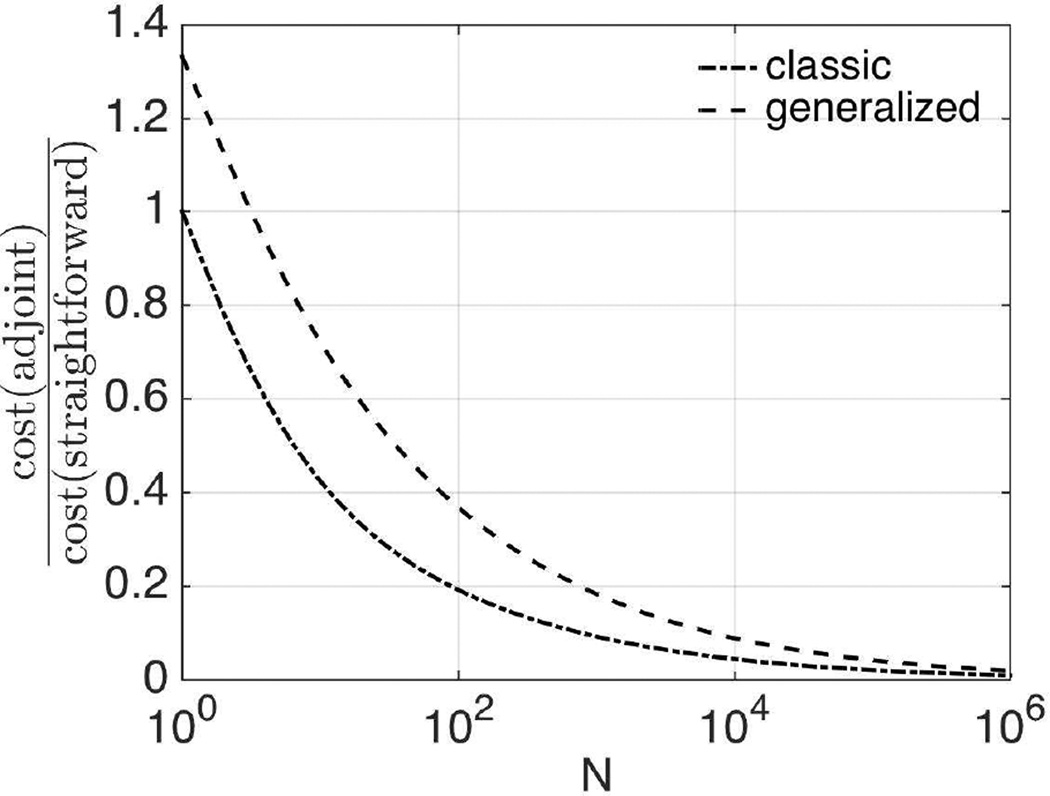
According to [41], the cost of solving the forward problem using Gaussian elimination is 𝒪(N^7/3) for LU factorization and 𝒪(N^5/3) for back-substitution, where N denotes the number of unknowns in the forward problem. Although the stiffness matrices in the force-driven and difference-driven equations take different forms, their sparse structures (thus the bandwidthes) are the same. In both the classic and generalized adjoint approaches, two forward solves are required. However, the LU factorization is carried out only once for the stiffness matrix K in the classic approach, while in the non-self-adjoint functional case, both K and K^⋆ need to be factorized. In the straightforward approach, the gradient vector g is estimated using (5)₁, which requires M + 1 forward solves. In addition, for the GN method, a linear system with a dense Hessian matrix H (4) needs to be solved in order to update the search direction, which costs 𝒪(N³). A summary of the computational cost for each iterative method is given in Table II. The straightforward approach requires M − 1 more back substitutions compared with the classic adjoint method. In both viscoelastic and poroelastic models studied in this work, M is the same order as N, thus the classic adjoint method takes 𝒪(N^5/3(N − 1)) fewer back-substitution operations than the straightforward approach. In FE implementation of phantom and human brain, N is between 10³ and 10⁶, implying substantial computational savings. The generalized adjoint approach requires factorization of both K and K^⋆, thus takes one more 𝒪(N^7/3) operation compared to the classic adjoint and straightforward methods. However, only two back-substitution steps are needed as in the classic adjoint approach, which leads to total savings of 𝒪(N^5/3(N − N^2/3 − 1)) operations compared with the straightforward calculation. Figure 1 shows theoretical estimates of the computational costs for the classic and generalized adjoint approaches compared with the straightforward calculation. Based on Table II, the values along the y-axis are

$$\frac{\text{cost}(\text{classic})}{\text{cost}(\text{straightforward})}=\frac{N^{2/3}+2}{N+N^{2/3}+1},$$ (55)

$$\frac{\text{cost}(\text{generalized})}{\text{cost}(\text{straightforward})}=\frac{2N^{2/3}+2}{N+N^{2/3}+1}$$

for the classic and generalized approaches, respectively, which converge to $1/N^{\frac{1}{3}}$ and $2/N^{\frac{1}{3}}$ as N tends to +∞. At N = 10³, the computational costs for the classic and generalized approaches are about 10% and 20% of that for the straightforward calculation, while at N = 10⁶, both approaches take less than 2% of the time in the straightforward approach.

TABLE II.

Computational costs per iteration.

method	computational cost
Gradient-based (classic adjoint)	𝒪(N7/3) + 2𝒪(N5/3)
Gradient-based (generalized adjoint)	2𝒪(N7/3) + 2𝒪(N5/3)
Gradient-based (straightforward)	𝒪(N7/3) + (M + 1)𝒪(N5/3)
Gauss-Newton	𝒪(N3) + 𝒪(N7/3) + (M + 1)𝒪(N5/3)

Fig. 1.

Theoretical cost estimates of the classic and generalized adjoint approaches compared with the straightforward gradient calculation based on LU decomposition and back substitution.

G. Parallel Computation

In this work, a sub-zone approach [29] is utilized in which the domain is divided into multiple overlapping sub-regions. Each processor is fully responsible for a small, complete iterative reconstruction task. This parallel scheme is easy to implement and has been shown to significantly reduce computational time. An iterative, reconstruction algorithm was developed with the Message Passing Interface (MPI) protocol in order to facilitate interprocess communication. Numerical studies presented in the following sections were performed on a 2600+ core Beowulf/Linux cluster. Forward problems were solved using multifrontal massively parallel sparse direct solver (MUMPS) [63], [64] owing to the sparse nature of the stiffness matrices.

III. Verification of the Generalized Adjoint Method

A. Phantom Study: Viscoelastic Modeling

A silicon phantom [65] was used in this study and consisted of a 50% A341 material background with cylindrical inclusions of four diameters - 29, 20, 15 and 10mm and four stiffness contrasts - 55, 60, 65 and 70% A341. All of the inclusions had an approximate thickness of 20mm and were arranged in three layers (16 inclusions in total). The cylindrical phantom had a slight taper from 90mm diameter at the base to 96mm at the top, and a height of 85mm. Displacement data were collected using a Philips 3T Achieva scanner (Philips Medical Systems Best, the Netherlands) with a single-shot, spin-echo echo-planar imaging sequence modified for MRE with motion sensitizing gradients and voxel size of 2mm×2mm×2mm. The phantom was vibrated using a piezoelectric actuator at 50Hz. Both viscoelastic models - (20) and (27) - and three optimization techniques - CG, QN and GN - were used to reconstruct the elastic properties of the phantom. Eqs. (20) and (27) are two equivalent forms of viscoelasticity; however, (27) provides a stabilized finite element form for the nearly incompressible case. In (20), λ estimates can be inaccurate since they are driven by the divergence term, ∇ · u, which is noisy in MR measurements. In order to implement (20), an upper bound on λ needs to be imposed for numerical stability. Previous studies [42], [34] have shown that both viscoelastic approaches are able to recover accurate shear moduli provided the longitudinal wave is modeled accurately.

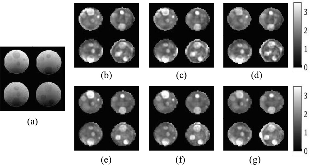
T2 image cross-sections and the corresponding reconstructed shear moduli are shown in Figure 2. The real and imaginary shear moduli are normally referred to as the storage and loss modulus, G′ and G″, respectively, in the dynamic modeling of complex materials where the loss modulus is related to the motion attenuation in the viscous case. The phantom was constructed from non-viscous silicon material; thus, only the real shear modulus was reconstructed in the inversion. Mechanical testing results of different A341 silicone concentrations given in [43] indicate that the storage modulus is essentially constant under different actuation freqencies, and varies from 3.3kPa for 50% A341 silicon gel and up to 11kPa for 100% A341 silicon gel. Our simulations predict reasonable ranges of shear moduli compared to these mechanical testing results.

Fig. 2.

Representative slices of reconstructed phantom properties. (a) T2 weighted image. (b–d) Real shear modulus in the compressible case using CG, QN and GN, respectively. (e–g) Real shear modulus in the incompressible case using CG, QN and GN, respectively. The shear modulus is displayed in units of kPa.

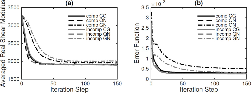
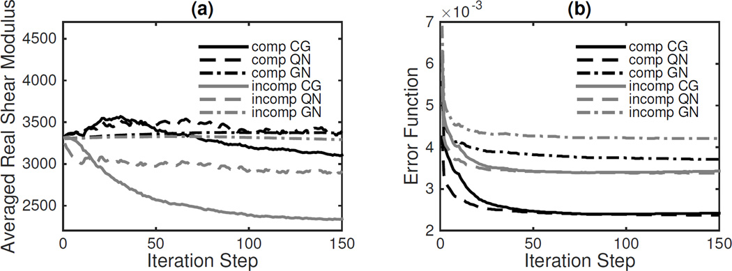
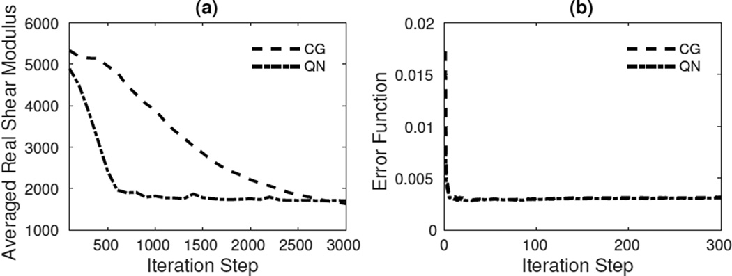
Figure 3 shows the averaged real shear modulus and a non-dimensionalized error function, γ, defined as

$$\mathrm{\gamma }=\frac{{\Vert {\mathit{u}}_c(\theta )-{\mathit{u}}_m\Vert }_{\mathrm{\Omega }}^2}{{\Vert {\mathit{u}}_m\Vert }_{\mathrm{\Omega }}^2}$$ (56)

for all iterations. QN converges slightly faster than CG, but the difference is small. The slower GN convergence is due to the added regularization of the Hessian.

Fig. 3.

Convergence results for compressible and incompressible viscoelastic models using CG, QN and GN methods in the Figure 2 phantom

B. Brain Study: Viscoelastic Modeling

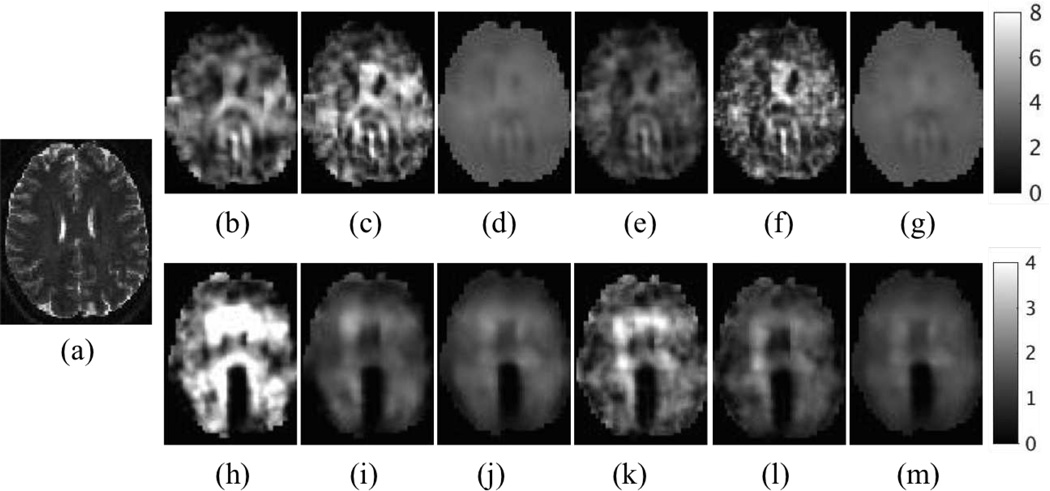
The brain has more complex microstructure relative to a phantom, and regions and structures can exhibit distinct mechanical properties. Here, externally actuated brain data was collected from a 24 year old healthy volunteer using a Siemens 3T Allegra scanner. Motion was applied at 50 Hz using a head rocker system, and a multishot, variable-density, spin-echo spiral MRE sequence was used to measure 3D displacements for 20 axial slices with voxel size of 2mm×2mm×2mm [32], [66]. Brain tissue is assumed to consist of viscoelastic solids and the elastic properties are reconstructed from MRE data using the same numerical methods as in the phantom study. The T2 weighted image of a healthy human brain is shown in Figure 4(a). The shear modulus images reconstructed with the compressible and incompressible models are presented in Figures 4(b–m). Similar to the findings from the phantom study, QN converges faster in general, compared to CG. Figure 5 shows the averaged shear modulus and error function convergence for the various method. Theoretically, GN converges faster because it incorporates second-order information. However, it suffers from a number of drawbacks:

• GN converges very slowly in practice because the Hessian matrix is heavily regularized to maintain numerical stability.

• GN increases computational time due to the inversion of a dense Hessian matrix, which is 𝒪(N³).

• GN requires memory storage of 𝒪(N²) for the dense matrix, which is one order of magnitude more than that for the gradient-based approaches.

Fig. 4.

Representative slices of reconstructed in vivo brain properties. (a) T2 weighted image. (b–d) Real shear modulus in the compressible case using CG, QN and GN, respectively. (e–g) Real shear modulus in the incompressible case using CG, QN and GN, respectively. (h–m) Imaginary shear moduli corresponding to their real counterparts in (b–g). The shear modulus is displayed in units of kPa.

Fig. 5.

Convergence results. Same as Figure 3, but for in vivo brain tissue MRE data from Figure 4.

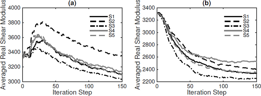
For these reasons, only CG and QN were applied in further in vivo studies. Lastly, to test the robustness of the numerical algorithm, five repeated MRI scans of the same subject were acquired. The averaged real shear moduli from CG are presented in Figure 6, where the computed shear moduli agree between 10–20% among the five scans.

Fig. 6.

Repeatibility tests of the reconstructed shear moduli from five MRE acquisitions (S1–S5) of the same subject. (a) Compressible Model; (b) Incompressible Model.

C. Phantom Study: Poroelastic Modeling

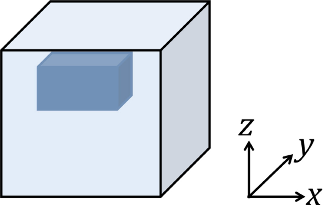
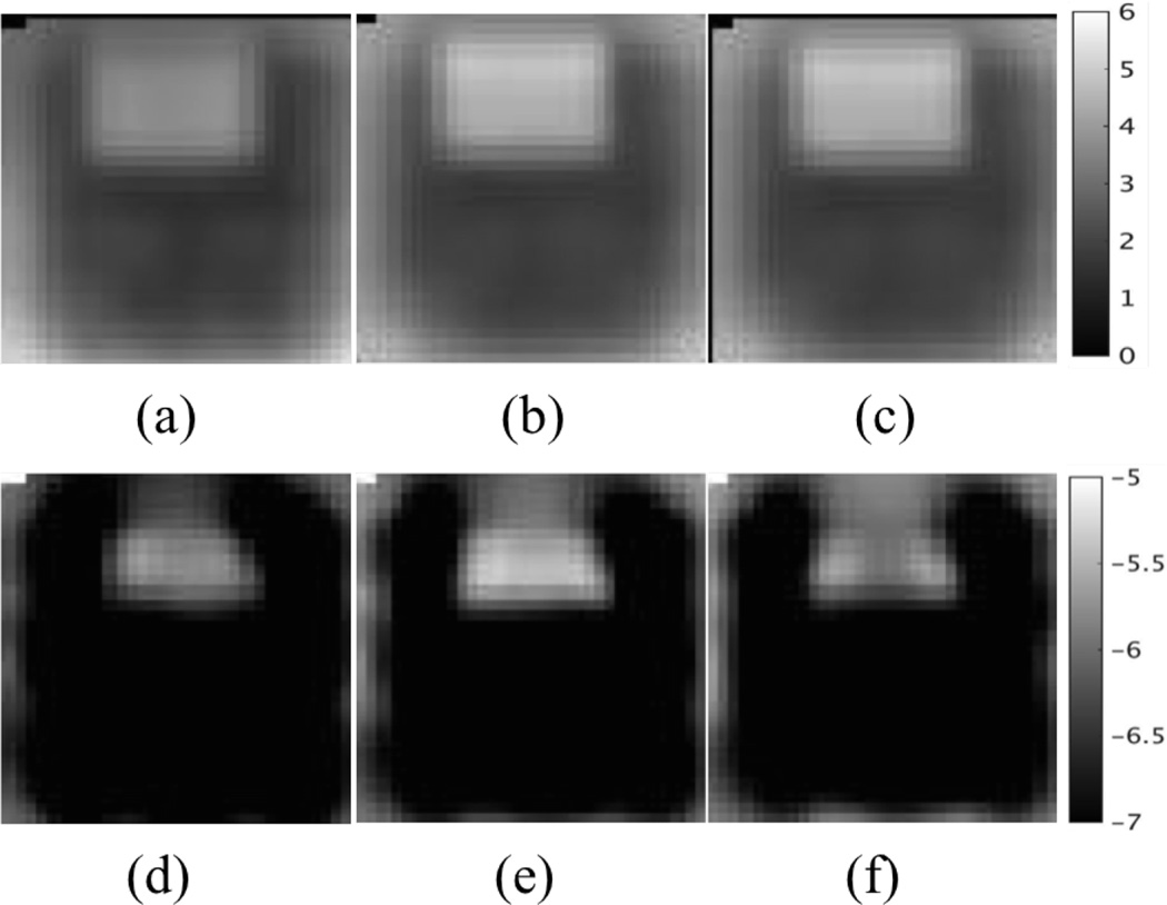
A simulated phantom with a single inclusion and a homogenous background was studied. The inclusion was located at the top of the homogenous matrix, as shown in Figure 7. The phantom was cube-shaped with edge length being 0.06m. The boundary conditions were set to be u=υ=w=0 on the top face, u=υ=0 and w=1e-4m on the bottom face, n · σ=0 on the rest of the faces and p=0 over all surfaces of the domain. The actuation frequency was set to be 1Hz, as used in intrinsic actuation MRE studies. By assuming a set of material properties including the shear modulus, the Lambda modulus, the hydraulic conductivity and the porosity for both the inclusion and the matrix (see Table III), a global forward problem was solved which computes the displacement and pressure fields based on the time-harmonic poroelastic model (31). The computed displacement values were then taken as measured data u_m, and an inverse problem was solved for material property distributions of μ, λ and κ. The reconstructed shear modulus and hydraulic conductivity images using CG, QN and GN methods are presented in Figure 8. The gradient calculation required in CG and QN was based on the generalized adjoint approach, while GN involves the conventional computation of the gradient vector. Consistency can be generally observed among the three iterative methods, indicating the feasibility of the proposed approach.

Fig. 7.

Illustrative picture of the simulated phantom consisting of a homogeneous background and a single inclusion.

TABLE III.

Material properties used in simulated phantom study.

material property	μ	λ	κ
matrix	3kPa	4.5kPa	1e–7m3s/Kg
inclusion	6kPa	9kPa	1e–5m3s/Kg

Fig. 8.

Representative slices of reconstructed material properties. (a–c) Real shear modulus using CG, QN and GN, respectively. (d–f) Real hydraulic conductivity using CG, QN and GN, respectively. The shear modulus is displayed in units of kPa, and the hydraulic conductivity is in units of m³s/kg and is presented in Logarithm scale.

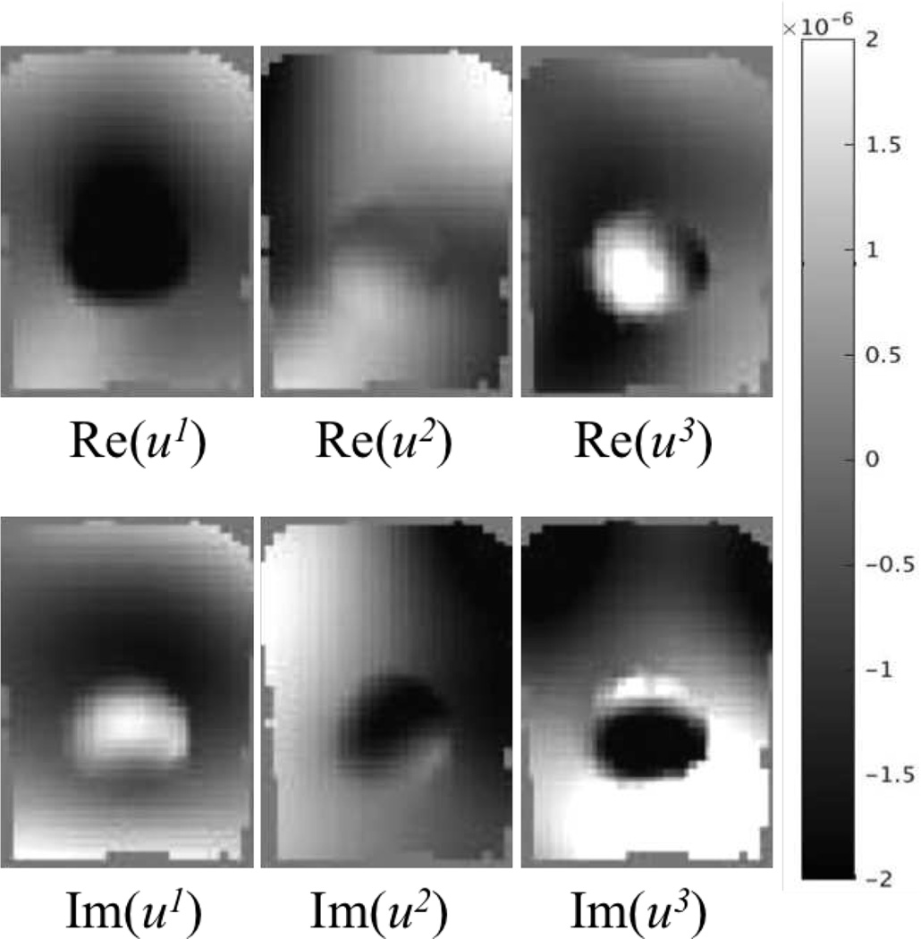
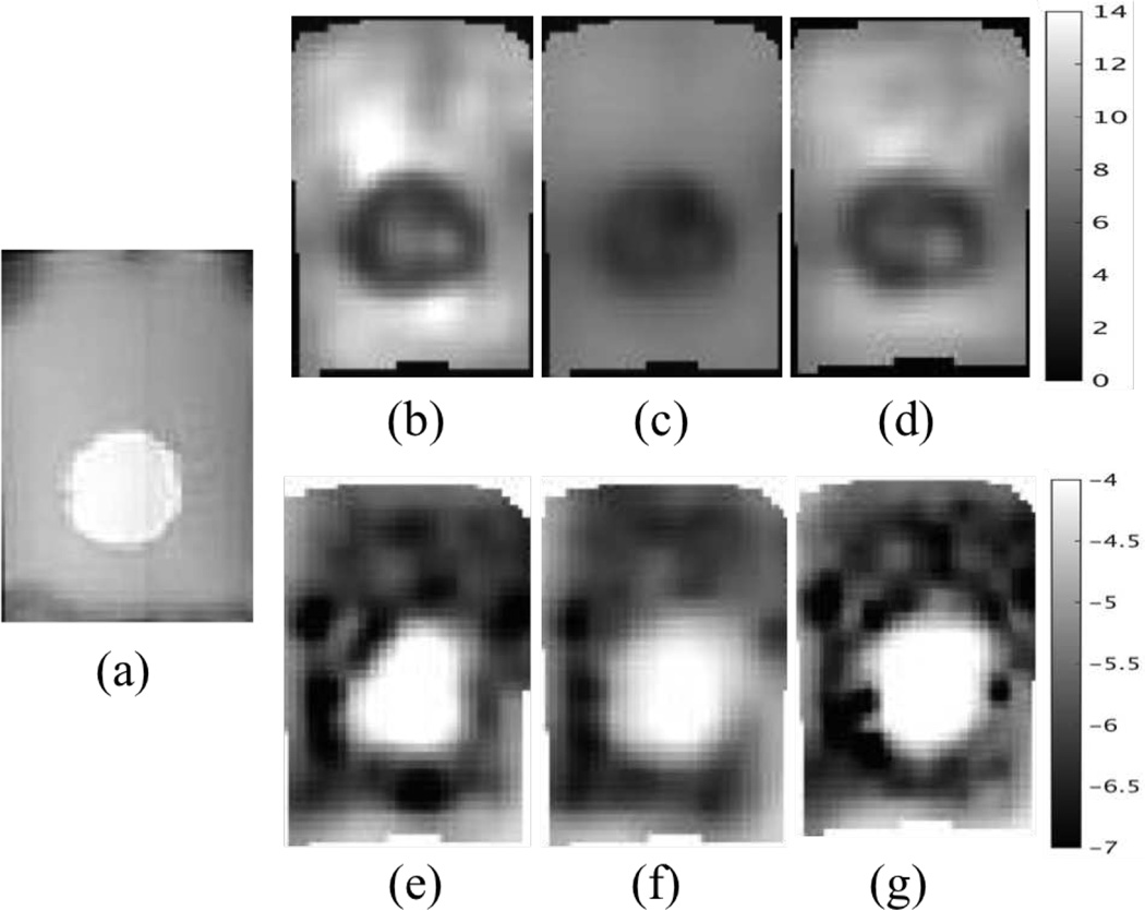
An experimental phantom was then investigated, in which a soft tofu inclusion was placed in an extra firm tofu background near the bottom of the background tofu. The phantom was vibrated at 50Hz with a piezoelectric actuator and the motion data were acquired on a Philips 3T Achieva MRI with voxel size 2mm×2mm×2mm. The displacement images of six components (i.e. the real and imaginary parts of u¹, u² and u³) are presented in Figure 9. Figure 10 shows the reconstructed shear modulus and hydraulic conductivity images from implementing CG, QN and GN. The results from CG and QN are consistent with those from GN. The inclusion has relatively lower stiffness and higher hydraulic conductivity. These findings agree well with poroelasticity-based dynamic mechanical analysis (DMA) results [67] reported in the literature.

Fig. 9.

Representative slices of displacement images of the experimental tofu at 50Hz.

Fig. 10.

Representative slices of reconstructed tofu properties. (a) T2 weighted image. (b–d) Real shear modulus using CG, QN and GN, respectively. (e–g) Real hydraulic conductivity using CG, QN and GN, respectively. The shear modulus is displayed in units of kPa, and the hydraulic conductivity is in units of m³s/kg and is presented in Logarithm scale.

D. Brain Study: Poroelastic Modeling

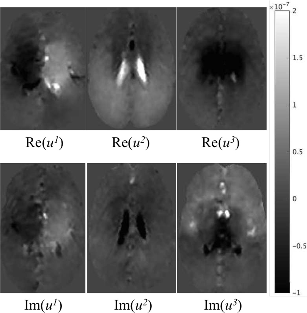
At low actuation frequencies, the viscous effect is small and the tissue deformation is mainly driven by bulk flow of interstitial fluid. Here, a multiphase, phase contrast, gradient echo, angiographic sequence recorded intrinsically generated displacements at 1Hz for a healthy volunteer corresponding to eight cardiac phases using retrospective gating synchronized to a pulse oximeter placed on the subject’s finger [19]. The acquired voxel size was 3mm×3mm×3mm, and 3D displacements for 16 slices centered around the ventricles were collected. Figure 11 shows representative displacement images from MRI acquisition. A poroelastic model was then adopted to estimate elastic brain tissue parameters with CG and QN reconstruction. Three parameters were reconstructed: the shear modulus μ; the Lambda modulus λ; and the hydraulic conductivity κ. Note that the imaginary parts of these parameters were set to be much lower than the magnitudes of the real parts in order to minimize viscous effects, although a more sophisticated poroviscoleastic model can be used at higher actuation frequencies.

Fig. 11.

Representative slices of displacement images of instrinsically activated brain.

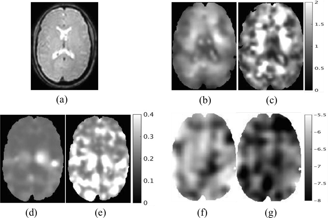
The T2 weighted image and material property reconstructions are shown in Figure 12. Both CG and QN methods capture the distinct features of the real shear modulus images very well, as given in Figure 12 (b–c). The real shear moduli images exhibit softening in the ventricular spaces due to the fluid components and bilateral periventricular increases in stiffness similar in structure to the viscoelastic patterns in Figure 4. The real Lambda moduli reconstructed from CG and QN are low and vaguely reconstructed, as shown in Figure 12 (d–e). The maximum values of λ_R are around 0.4kPa and 0.7kPa, respectively. These results are not unexpected due to the insensitivity of the measured displacements to this parameter. The hydraulic conductivity images in Figure 12 (f–g) show fairly uniform values around 1e-5.5 except for two ‘dark’ regions nearly symmetric with respect to the ventricles probably due to the presence of thalamus and putamen.

Fig. 12.

Representative slices of reconstructed in vivo brain properties. (a) T2 weighted image. (b–c) Real shear modulus using CG and QN, respectively. (d–e) Real Lambda modulus using CG and QN, respectively. (f–g) Real hydraulic conductivity using CG and QN, respectively. All of the results are based on poroelastic model under intrinsic actuation. The shear and Lambda moduli are displayed in units of kPa, and the hydraulic conductivity is in units of m³s/kg and is presented in Logarithm scale.

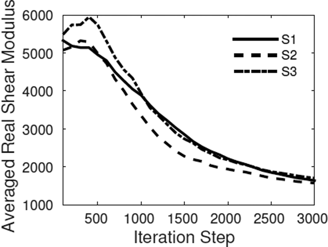
Convergence results of CG and QN are given in Figure 13. As in the viscoelastic case, QN converges faster than CG to a mean shear modulus around 2kPa in both cases, which is lower than the mean values (between 2.5kPa and 3.5kPa) found at 50Hz. This observation is consistent with the frequency dependence of human brain shear modulus reported in [68]. However, the poroelastic reconstruction takes an order of magnitude more iterations to converge than the externally actuated viscoelastic model. The longer convergence may be due to the more difficult task of matching the measured motions while maintaining a reasonable pressure gradient distribution within the model. Repeatability tests using MRI scans were also evaluated and the averaged shear moduli from three scans of the same subject agree well with one another, as shown in Figure 14, indicating that some stable absolute shear modulus value has been achieved in the low frequency regime.

Fig. 13.

Convergence results. Same as Figures 3 and 5, but for intrinsic MRE data from Figure 12.

Fig. 14.

Repeatibility tests of the reconstructed shear moduli from three intrinsic MRE acquistions (S1–S3) of the same subject.

E. Simulation Time

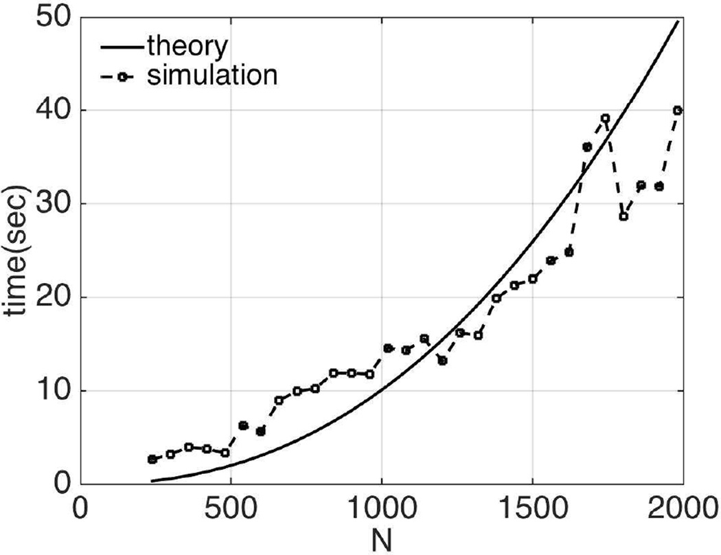
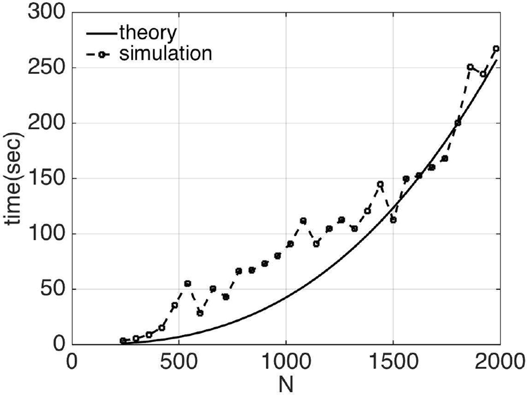
In this section, the relation between the numerical simulation time using the generalized adjoint approach and the size of the forward problem, N, is investigated, and compared with the theoretically estimated values in Section II-F. Here, CG is applied for updating the material properties of the experimental phantom in Section III-C. The forward problem size, N, is controlled by the size of subzones. A number of different problem sizes varying from 240 to 2000 were studied. The results are given in Figure 15. Theoretically, the computational time is proportional to N^7/3+N^5/3. The corresponding data for the straightforward approach are shown in Figure 16. In this case, the number of parameters to be reconstructed is M=3N/4; therefore, the computational cost is 𝒪(3/4N^8/3+N^7/3+N^5/3). The actual simulation times follow the theoretical trends in both cases.

Fig. 15.

Comparison of computational costs from theoretical estimation and numerical simulation vs. size of the forward problem using the generalized adjoint approach in the poroelastic model.

Fig. 16.

Comparison of computational costs from theoretical estimation and numerical simulation vs. size of the forward problem using the straightforward approach in the poroelastic model.

IV. Conclusions

Efficient algorithms for gradient calculation in the MRE inversion process are presented in this study. The approach is based on a Lagrangian method to derive a difference-driven forward problem without requiring a self-adjoint functional, A(δW, U; θ), from the force-driven forward problem. Thus, this method can be regarded as a generalized ‘adjoint method’ that is applicable to a wide range of inverse problems. The gradient computation is as efficient as in the classic self-adjoint approach, using only two sparse matrix solutions which are independent of the number of estimation parameters. Numerical implementation of the approach in poroelastic MRE is also demonstrated, including a linear system of adjoint finite element equations and discrete forms of the gradient vector with respect to the parameters to be reconstructed.

Our results show that by applying the generalized adjoint method in gradient-based optimization algorithms, reasonable material property distribution images can be generated in phantom and brain tissue. Moreover, the relationship between the numerical simulation time in the generalized approach and the forward problem size is consistent with the theoretical estimation. Our approach is readily extended to other medical imaging problems in which the non-self-adjoint form arises, either from the nonlinearity of the problem [69] or from the coupling of different physical fields [70].

Appendix A

Viscoelastic Model: Compressible Case

First we derive the discrete system for the force-driven forward problem (22). Let us denote the finite element approximated functions to be

$$\mathit{u}={(u^1,u^2,u^3)}^T,\delta \mathit{\upsilon }={(\delta {\upsilon }^1,\delta {\upsilon }^2,\delta {\upsilon }^3)}^T,$$ (A.1)

where (u¹, u², u³) and (δυ¹, δυ², δυ³) indicate the three components of the displacement field in the trial function and test function spaces, respectively. The finite element discretization gives

$$\mathit{u}={\mathit{u}}_k{\varphi }_k,\delta \mathit{\upsilon }=\delta {\mathit{\upsilon }}_j{\varphi }_j.$$ (A.2)

The discretized terms in A (u, δυ; θ) are

$$(\nabla \mathit{u}:\mathit{I})\mathit{I}:\nabla \mathit{\delta }\mathit{\upsilon }=(u_k^1\frac{\partial {\varphi }_k}{\partial x}+u_k^2\frac{\partial {\varphi }_k}{\partial y}+u_k^3\frac{\partial {\varphi }_k}{\partial z})·(\delta {\upsilon }_j^1\frac{\partial {\varphi }_j}{\partial x}+\delta {\upsilon }_j^2\frac{\partial {\varphi }_j}{\partial y}+\delta {\upsilon }_j^3\frac{\partial {\varphi }_j}{\partial z}),$$ (A.3)

$$\nabla \mathit{u}:\nabla \delta \mathit{\upsilon }=(u_k^1\delta {\upsilon }_j^1+u_k^2\delta {\upsilon }_j^2+u_k^3\delta {\upsilon }_j^3)·(\frac{\partial {\varphi }_k}{\partial x}\frac{\partial {\varphi }_j}{\partial x}+\frac{\partial {\varphi }_k}{\partial y}\frac{\partial {\varphi }_j}{\partial y}+\frac{\partial {\varphi }_k}{\partial z}\frac{\partial {\varphi }_j}{\partial z}),$$ (A.4)

$$\nabla {\mathit{u}}^T:\nabla \delta \mathit{\upsilon }=(u_k^1\frac{\partial {\varphi }_j}{\partial x}+u_k^2\frac{\partial {\varphi }_j}{\partial y}+u_k^3\frac{\partial {\varphi }_j}{\partial z})·(\delta {\upsilon }_j^1\frac{\partial {\varphi }_k}{\partial x}+\delta {\upsilon }_j^2\frac{\partial {\varphi }_k}{\partial y}+\delta {\upsilon }_j^3\frac{\partial {\varphi }_k}{\partial z}),$$ (A.5)

$$\mathit{u}·\delta \mathit{\upsilon }=(u_k^1\delta {\upsilon }_j^1+u_k^2\delta {\upsilon }_j^2+u_k^3\delta {\upsilon }_j^3){\varphi }_k{\varphi }_j.$$ (A.6)

From (15) and (A.3), we can derive a linear system

$$[\mathit{K}]\{\mathit{u}\}=\{f\}$$ (A.7)

with the elements of the stiffness matrix K and the forcing vector f being

$$K_{3(j-1)+1,3(k-1)+1}=\langle (2\mu +\lambda )\frac{\partial {\varphi }_k}{\partial x}\frac{\partial {\varphi }_j}{\partial x}+\mu (\frac{\partial {\varphi }_k}{\partial y}\frac{\partial {\varphi }_j}{\partial y}+\frac{\partial {\varphi }_k}{\partial z}\frac{\partial {\varphi }_j}{\partial z})-{\omega }^2\rho {\varphi }_k{\varphi }_j\rangle ,$$

$$K_{3(j-1)+2,3(k-1)+2}=\langle (2\mu +\lambda )\frac{\partial {\varphi }_k}{\partial y}\frac{\partial {\varphi }_j}{\partial y}+\mu (\frac{\partial {\varphi }_k}{\partial x}\frac{\partial {\varphi }_j}{\partial x}+\frac{\partial {\varphi }_k}{\partial z}\frac{\partial {\varphi }_j}{\partial z})-{\omega }^2\rho {\varphi }_k{\varphi }_j\rangle ,$$ (A.8)

$$K_{3(j-1)+3,3(k-1)+3}=\langle (2\mu +\lambda )\frac{\partial {\varphi }_k}{\partial z}\frac{\partial {\varphi }_j}{\partial z}+\mu (\frac{\partial {\varphi }_k}{\partial x}\frac{\partial {\varphi }_j}{\partial x}+\frac{\partial {\varphi }_k}{\partial y}\frac{\partial {\varphi }_j}{\partial y})-{\omega }^2\rho {\varphi }_k{\varphi }_j\rangle ,$$

$$K_{3(j-1)+1,3(k-1)+2}=K_{3(j-1)+2,3(k-1)+1}=\langle \lambda \frac{\partial {\varphi }_k}{\partial y}\frac{\partial {\varphi }_j}{\partial x}+\mu \frac{\partial {\varphi }_k}{\partial x}\frac{\partial {\varphi }_j}{\partial y}\rangle ,$$

$$K_{3(j-1)+1,3(k-1)+3}=K_{3(j-1)+3,3(k-1)+1}=\langle \lambda \frac{\partial {\varphi }_k}{\partial z}\frac{\partial {\varphi }_j}{\partial x}+\mu \frac{\partial {\varphi }_k}{\partial x}\frac{\partial {\varphi }_j}{\partial z}\rangle ,$$ (A.9)

$$K_{3(j-1)+2,3(k-1)+3}=K_{3(j-1)+3,3(k-1)+2}=\langle \lambda \frac{\partial {\varphi }_k}{\partial z}\frac{\partial {\varphi }_j}{\partial y}+\mu \frac{\partial {\varphi }_k}{\partial y}\frac{\partial {\varphi }_j}{\partial z}\rangle .$$

and

$$f_{3(j-1)+1}={\mathit{n}}_x·{\oint }_{{\mathrm{\Gamma }}_{\sigma }}{\mathit{f}}_0{\varphi }_{j}d{\mathrm{\Gamma }}_{\sigma },$$

$$f_{3(j-1)+2}={\mathit{n}}_y·{\oint }_{{\mathrm{\Gamma }}_{\sigma }}{\mathit{f}}_0{\varphi }_{j}d{\mathrm{\Gamma }}_{\sigma },$$ (A.10)

$$f_{3(j-1)+3}={\mathit{n}}_z·{\oint }_{{\mathrm{\Gamma }}_{\sigma }}{\mathit{f}}_0{\varphi }_{j}d{\mathrm{\Gamma }}_{\sigma }.$$

We denote the difference-driven forward problem as

$$[{\mathit{K}}^{\star }]\{\mathit{\upsilon }\}=\{f^{\star }\},$$ (A.11)

where we can simply check that K^⋆ = K, with forcing terms

$$f_{3(j-1)+1}^{\star }=-{(u_j^1-{(u_m)}_j^1)}^H,$$

$$f_{3(j-1)+2}^{\star }=-{(u_j^2-{(u_m)}_j^2)}^H,$$ (A.12)

$$f_{3(j-1)+3}^{\star }=-{(u_j^3-{(u_m)}_j^3)}^H.$$

Now let us look at the calculation of the gradient vector. In the compressible case, the material properties, θ, include Lamé’s first and second parameters, λ and μ. The reader is referred to [57] for more detail. Let us denote

$$\theta ={(\lambda ,\mu )}^T=\sum _{j=1}^{N_{\theta }}{\theta }_j{\mathit{e}}_j,$$ (A.13)

where N_θ represents the number of material properties, θ_j indicates the j-th number of the material property and e_j is a unit vector in j-th direction. In our case, N_θ is equal to 2; λ and μ are denoted by θ₁ and θ₂, respectively. The discrete form for each θ_j is given by

$${\theta }_j=\sum _{n=1}^{N_{\text{nodes}}}{\varphi }_n(x,y,z)b_{jn}.$$ (A.14)

In the above equation, N_nodes denotes the total number of nodes in the finite element mesh; ϕ_n(x, y, z) refers to the shape function of the n-th node and b_jn is the value of the j-th material property at the node n. Similarly, the variations in θ can be written as

$$\delta {\theta }_j=\sum _{n=1}^{N_{\text{nodes}}}{\varphi }_n(x,y,z)\delta b_{jn}.$$ (A.15)

From (A.13) and (A.15), we have

$$\delta \theta =\sum _{j=1}^{N_{\theta }}\delta {\theta }_j{\mathit{e}}_j=\sum _{j=1}^{N_{\theta }}\sum _{n=1}^{N_{\text{nodes}}}{\varphi }_n(x,y,z)\delta b_{jn}{\mathit{e}}_j.$$ (A.16)

Using the above equations, we shall find the discrete formulation of (17). From (A.13), we can write

$$\lambda =\theta ·{\mathit{e}}_1,\mu =\theta ·{\mathit{e}}_2.$$ (A.17)

Substituting (A.17) and (25) into (17) leads to

$$\delta \mathrm{\Pi }={\int }_{\mathrm{\Omega }}({\mathit{e}}_1·\delta \theta )(\nabla \mathit{u}:\mathit{I})\mathit{I}:\nabla \mathit{\upsilon }+({\mathit{e}}_2·\delta \theta )(\nabla \mathit{u}+\nabla {\mathit{u}}^T):\nabla \mathit{\upsilon }d\mathrm{\Omega }.$$ (A.18)

Furthermore, substituting (A.16) into (A.18) gives rise to

$$\delta \mathrm{\Pi }=\sum _{j=1}^{N_{\theta }}\sum _{n=1}^{N_{\text{nodes}}}\delta b_{jn}({\delta }_{1j}{\int }_{\mathrm{\Omega }}{\varphi }_n(x,y,z)(\nabla \mathit{u}:\mathit{I})\mathit{I}:\nabla \mathit{\upsilon }+{\delta }_{2j}{\int }_{\mathrm{\Omega }}{\varphi }_n(x,y,z)(\nabla \mathit{u}+\nabla {\mathit{u}}^T):\nabla \mathit{\upsilon }d\mathrm{\Omega }),$$ (A.19)

where δ_1j and δ_2j are the Kronecker’s delta functions. Based on the definition of the gradient vector, we also have

$$\delta \mathrm{\Pi }=\sum _{j=1}^{N_{\theta }}\sum _{n=1}^{N_{\text{nodes}}}{g}_{jn}\delta b_{jn}.$$ (A.20)

Therefore, the gradient vector is taken to be

$$g_{jn}={\delta }_{1j}{\int }_{\mathrm{\Omega }}{\varphi }_n(x,y,z)(\nabla \mathit{u}:\mathit{I})\mathit{I}:\nabla \mathit{\upsilon }+{\delta }_{2j}{\int }_{\mathrm{\Omega }}{\varphi }_n(x,y,z)(\nabla \mathit{u}+\nabla {\mathit{u}}^T):\nabla \mathit{\upsilon }d\mathrm{\Omega }.$$ (A.21)

Alternatively,

$$g_{1n}=\frac{\partial \mathrm{\Pi }}{\partial {\lambda }_n}={\int }_{\mathrm{\Omega }}{\varphi }_n(x,y,z)(\nabla \mathit{u}:\mathit{I})\mathit{I}:\nabla \mathit{\upsilon }d\mathrm{\Omega },$$ (A.22)

$$g_{2n}=\frac{\partial \mathrm{\Pi }}{\partial {\mu }_n}={\int }_{\mathrm{\Omega }}{\varphi }_n(x,y,z)(\nabla \mathit{u}+\nabla {\mathit{u}}^T):\nabla \mathit{\upsilon }d\mathrm{\Omega }.$$

We present the numerical algorithm for gradient calculation below:

1. Solve the force-driven forward problem (A.7);

2. Solve the difference-driven forward problem (A.11);

3. Compute the gradient using (A.22).

Appendix B

Viscoelastic Model: Incompressible Case

We only present the extra terms in (29) compared to the compressible case, which are

$$p\mathit{I}:\nabla \delta \mathit{\upsilon }=(\frac{\partial {\varphi }_j}{\partial x}\delta {\upsilon }_j^1+\frac{\partial {\varphi }_j}{\partial y}\delta {\upsilon }_j^2+\frac{\partial {\varphi }_j}{\partial z}\delta {\upsilon }_j^3)p_k{\varphi }_k,$$ (B.1)

$$(\nabla ·\mathit{u})\delta q=(\frac{\partial {\varphi }_k}{\partial x}{u}_k^1+\frac{\partial {\varphi }_k}{\partial y}{u}_k^2+\frac{\partial {\varphi }_k}{\partial z}{u}_k^3)\delta q_j{\varphi }_j,p\delta q={\varphi }_k{\varphi }_j{p}_k\delta q_j.$$

The 3 × 3 sub-matrix in the stiffness matrix K as in the compressible case is given by

$$K_{4(j-1)+1,4(k-1)+1}=\langle 2\mu \frac{\partial {\varphi }_k}{\partial x}\frac{\partial {\varphi }_j}{\partial x}+\mu (\frac{\partial {\varphi }_k}{\partial y}\frac{\partial {\varphi }_j}{\partial y}+\frac{\partial {\varphi }_k}{\partial z}\frac{\partial {\varphi }_j}{\partial z})-{\omega }^2\rho {\varphi }_k{\varphi }_j\rangle ,$$

$$K_{4(j-1)+2,4(k-1)+2}=\langle 2\mu \frac{\partial {\varphi }_k}{\partial y}\frac{\partial {\varphi }_j}{\partial y}+\mu (\frac{\partial {\varphi }_k}{\partial x}\frac{\partial {\varphi }_j}{\partial x}+\frac{\partial {\varphi }_k}{\partial z}\frac{\partial {\varphi }_j}{\partial z})-{\omega }^2\rho {\varphi }_k{\varphi }_j\rangle ,$$ (B.2)

$$K_{4(j-1)+3,4(k-1)+3}=\langle 2\mu \frac{\partial {\varphi }_k}{\partial z}\frac{\partial {\varphi }_j}{\partial z}+\mu (\frac{\partial {\varphi }_k}{\partial x}\frac{\partial {\varphi }_j}{\partial x}+\frac{\partial {\varphi }_k}{\partial y}\frac{\partial {\varphi }_j}{\partial y})-{\omega }^2\rho {\varphi }_k{\varphi }_j\rangle$$

$$K_{4(j-1)+1,4(k-1)+2}=K_{4(j-1)+2,4(k-1)+1}=\langle \mu \frac{\partial {\varphi }_k}{\partial x}\frac{\partial {\varphi }_j}{\partial y}\rangle ,$$

$$K_{4(j-1)+1,4(k-1)+3}=K_{4(j-1)+3,4(k-1)+1}=\langle \mu \frac{\partial {\varphi }_k}{\partial x}\frac{\partial {\varphi }_j}{\partial z}\rangle ,$$

$$K_{4(j-1)+2,4(k-1)+3}=K_{4(j-1)+3,4(k-1)+2}=\langle \mu \frac{\partial {\varphi }_k}{\partial y}\frac{\partial {\varphi }_j}{\partial z}\rangle .$$ (B.3)

The rest of the components are

$$K_{4(j-1)+1,4(k-1)+4}=-{\varphi }_k\frac{\partial {\varphi }_j}{\partial x},$$

$$K_{4(j-1)+4,4(k-1)+1}=-\frac{\partial {\varphi }_k}{\partial x}{\varphi }_j,$$

$$K_{4(j-1)+2,4(k-1)+4}=-{\varphi }_k\frac{\partial {\varphi }_j}{\partial y},$$

$$K_{4(j-1)+4,4(k-1)+2}=-\frac{\partial {\varphi }_k}{\partial y}{\varphi }_j,$$ (B.4)

$$K_{4(j-1)+3,4(k-1)+4}=-{\varphi }_k\frac{\partial {\varphi }_j}{\partial z},$$

$$K_{4(j-1)+4,4(k-1)+3}=-\frac{\partial {\varphi }_k}{\partial z}{\varphi }_j,$$

$$K_{4(j-1)+4,4(k-1)+4}=-\frac{{\varphi }_k{\varphi }_j}{K}.$$

The forcing term f and the adjoint forcing term f^⋆ are

$$f_{4(j-1)+1}={\mathit{n}}_x·{\oint }_{{\mathrm{\Gamma }}_{\sigma }}{\mathit{f}}_0{\varphi }_{j}d{\mathrm{\Gamma }}_{\sigma },$$

$$f_{4(j-1)+2}={\mathit{n}}_y·{\oint }_{{\mathrm{\Gamma }}_{\sigma }}{\mathit{f}}_0{\varphi }_{j}d{\mathrm{\Gamma }}_{\sigma },$$ (B.5)

$$f_{4(j-1)+3}={\mathit{n}}_z·{\oint }_{{\mathrm{\Gamma }}_{\sigma }}{\mathit{f}}_0{\varphi }_{j}d{\mathrm{\Gamma }}_{\sigma },$$

$$f_{4(j-1)+4}=0$$

and

$$f_{4(j-1)+1}^{\star }=-{(u_j^1-{(u_m)}_j^1)}^H,$$

$$f_{4(j-1)+2}^{\star }=-{(u_j^2-{(u_m)}_j^2)}^H,$$ (B.6)

$$f_{4(j-1)+3}^{\star }=-{(u_j^3-{(u_m)}_j^3)}^H,$$

$$f_{4(j-1)+4}^{\star }=0.$$

Note that in the incompressible case, only the shear modulus needs to be reconstructed, thus we take (A.22)₂ as the gradient vector.

Appendix C

Poroelastic Model

First, the discrete system of the force-driven forward problem in (15) is derived by denoting the finite element approximation through

$$U={(\mathit{u},p)}^T={(u^1,u^2,u^3,p)}^T,$$ (C.1)

$$\delta W={(\delta \mathit{\upsilon },\delta q)}^T={(\delta {\upsilon }^1,\delta {\upsilon }^2,\delta {\upsilon }^3,\delta q)}^T,$$

where (u¹, u², u³) and (δυ¹, δυ², δυ³) are the three components of the displacement field defined in 𝒮 and 𝒱, respectively. The finite element discretization yields

$$U=U_k{\varphi }_k,\delta W=\delta W_j{\varphi }_j.$$ (C.2)

where the terms that are new in the poroelastic model are

$$\nabla p·\delta \mathit{\upsilon }=(\delta {\upsilon }_j^1\frac{\partial {\varphi }_k}{\partial x}+\delta {\upsilon }_j^2\frac{\partial {\varphi }_k}{\partial y}+\delta {\upsilon }_j^3\frac{\partial {\varphi }_k}{\partial z})p_k{\varphi }_j,$$

$$(\nabla ·\mathit{u})\delta q=(u_k^1\frac{\partial {\varphi }_k}{\partial x}+u_k^2\frac{\partial {\varphi }_k}{\partial y}+u_k^3\frac{\partial {\varphi }_k}{\partial z})\delta q_j{\varphi }_j,$$ (C.3)

$$\mathit{u}·\nabla \delta q=(u_k^1\frac{\partial {\varphi }_j}{\partial x}+u_k^2\frac{\partial {\varphi }_j}{\partial y}+u_k^3\frac{\partial {\varphi }_j}{\partial z})\delta q_j{\varphi }_k,$$

$$\nabla p·\nabla \delta p=(\frac{\partial {\varphi }_k}{\partial x}\frac{\partial {\varphi }_j}{\partial x}+\frac{\partial {\varphi }_k}{\partial y}\frac{\partial {\varphi }_j}{\partial y}+\frac{\partial {\varphi }_k}{\partial z}\frac{\partial {\varphi }_j}{\partial z})p_k\delta q_j.$$

As in the viscoelastic case, a linear system is given as

$$[\mathit{K}]\{U\}=\{f\},$$ (C.4)

results in elements of the stiffness matrix, K, and the forcing vector, f, consistent with [44], [45]. Diagonal terms in the stiffness matrix are given by

$$K_{4(j-1)+1,4(k-1)+1}=\langle (2\mu +\lambda )\frac{\partial {\varphi }_k}{\partial x}\frac{\partial {\varphi }_j}{\partial x}+\mu (\frac{\partial {\varphi }_k}{\partial y}\frac{\partial {\varphi }_j}{\partial y}+\frac{\partial {\varphi }_k}{\partial z}\frac{\partial {\varphi }_j}{\partial z})-{\omega }^2(\rho -\beta {\rho }_f){\varphi }_k{\varphi }_j\rangle ,$$

$$K_{4(j-1)+2,4(k-1)+2}=\langle (2\mu +\lambda )\frac{\partial {\varphi }_k}{\partial y}\frac{\partial {\varphi }_j}{\partial y}+\mu (\frac{\partial {\varphi }_k}{\partial x}\frac{\partial {\varphi }_j}{\partial x}+\frac{\partial {\varphi }_k}{\partial z}\frac{\partial {\varphi }_j}{\partial z})-{\omega }^2(\rho -\beta {\rho }_f){\varphi }_k{\varphi }_j\rangle ,$$

$$K_{4(j-1)+3,4(k-1)+3}=\langle (2\mu +\lambda )\frac{\partial {\varphi }_k}{\partial z}\frac{\partial {\varphi }_j}{\partial z}+\mu (\frac{\partial {\varphi }_k}{\partial x}\frac{\partial {\varphi }_j}{\partial x}+\frac{\partial {\varphi }_k}{\partial y}\frac{\partial {\varphi }_j}{\partial y})-{\omega }^2(\rho -\beta {\rho }_f){\varphi }_k{\varphi }_j\rangle ,$$

$$K_{4(j-1)+4,4(k-1)+4}=\langle -\frac{i\beta }{\omega {\rho }_f}(\frac{\partial {\varphi }_k}{\partial x}\frac{\partial {\varphi }_j}{\partial x}+\frac{\partial {\varphi }_k}{\partial y}\frac{\partial {\varphi }_j}{\partial y}+\frac{\partial {\varphi }_k}{\partial z}\frac{\partial {\varphi }_j}{\partial z})\rangle ;$$ (C.5)

the sub-matrix elements from elasticity are symmetric, thus the off-diagonal contributions can be written as

$$K_{4(j-1)+1,4(k-1)+2}=K_{4(j-1)+2,4(k-1)+1}=\langle \lambda \frac{\partial {\varphi }_k}{\partial y}\frac{\partial {\varphi }_j}{\partial x}+\mu \frac{\partial {\varphi }_k}{\partial x}\frac{\partial {\varphi }_j}{\partial y}\rangle ,$$

$$K_{4(j-1)+1,4(k-1)+3}=K_{4(j-1)+3,4(k-1)+1}=\langle \lambda \frac{\partial {\varphi }_k}{\partial z}\frac{\partial {\varphi }_j}{\partial x}+\mu \frac{\partial {\varphi }_k}{\partial x}\frac{\partial {\varphi }_j}{\partial z}\rangle ,$$ (C.6)

$$K_{4(j-1)+2,4(k-1)+3}=K_{4(j-1)+3,4(k-1)+2}=\langle \lambda \frac{\partial {\varphi }_k}{\partial z}\frac{\partial {\varphi }_j}{\partial y}+\mu \frac{\partial {\varphi }_k}{\partial y}\frac{\partial {\varphi }_j}{\partial z}\rangle ;$$

whereas the off-diagonal entries from the pressure equation become

$$K_{4(j-1)+1,4(k-1)+4}=\langle (1-\beta )\frac{\partial {\varphi }_k}{\partial x}{\varphi }_j\rangle ,$$

$$K_{4(j-1)+4,4(k-1)+1}=\langle i\omega (\frac{\partial {\varphi }_k}{\partial x}{\varphi }_j+\beta {\varphi }_k\frac{\partial {\varphi }_j}{\partial x})\rangle ,$$

$$K_{4(j-1)+2,4(k-1)+4}=\langle (1-\beta )\frac{\partial {\varphi }_k}{\partial y}{\varphi }_j\rangle ,$$ (C.7)

$$K_{4(j-1)+4,4(k-1)+2}=\langle i\omega (\frac{\partial {\varphi }_k}{\partial y}{\varphi }_j+\beta {\varphi }_k\frac{\partial {\varphi }_j}{\partial y})\rangle ,$$

$$K_{4(j-1)+3,4(k-1)+4}=\langle (1-\beta )\frac{\partial {\varphi }_k}{\partial z}{\varphi }_j\rangle ,$$

$$K_{4(j-1)+4,4(k-1)+3}=\langle i\omega (\frac{\partial {\varphi }_k}{\partial z}{\varphi }_j+\beta {\varphi }_k\frac{\partial {\varphi }_j}{\partial z})\rangle .$$

Finally, the forcing vector is given by

$$f_{4(j-1)+1}={\mathit{n}}_x·{\oint }_{\mathrm{\Gamma }}{\mathit{f}}_0{\varphi }_{j}d\mathrm{\Gamma },$$

$$f_{4(j-1)+2}={\mathit{n}}_y·{\oint }_{\mathrm{\Gamma }}{\mathit{f}}_0{\varphi }_{j}d\mathrm{\Gamma },$$ (C.8)

$$f_{4(j-1)+3}={\mathit{n}}_z·{\oint }_{\mathrm{\Gamma }}{\mathit{f}}_0{\varphi }_{j}d\mathrm{\Gamma },$$

$$f_{4(j-1)+4}={\oint }_{\mathrm{\Gamma }}{r}_0{\varphi }_{j}d\mathrm{\Gamma }.$$

Note that 〈·〉 indicates volume integration over the local element; n_x, n_y and n_z refer to the unit vector outwardly normal to the surface in the x, y and z direction, respectively.

References

- 1.Huwart L, Sempoux C, Vicaut E, Salameh N, Annet L, Danse E, Peeters F, ter Beek LC, Rahier J, Sinkus R, et al. Magnetic resonance elastography for the noninvasive staging of liver fibrosis. Gastroenterology. 2008;135(1):32–40. doi: 10.1053/j.gastro.2008.03.076. [DOI] [PubMed] [Google Scholar]
- 2.Chen J, Talwalkar JA, Yin M, Glaser KJ, Sanderson SO, Ehman RL. Early detection of nonalcoholic steatohepatitis in patients with nonalcoholic fatty liver disease by using mr elastography. Radiology. 2011;259(3):749–756. doi: 10.1148/radiol.11101942. [DOI] [PMC free article] [PubMed] [Google Scholar]
- 3.Asbach P, Klatt D, Hamhaber U, Braun J, Somasundaram R, Hamm B, Sack I. Assessment of liver viscoelasticity using multifrequency mr elastography. Magnetic Resonance in Medicine. 2008;60(2):373–379. doi: 10.1002/mrm.21636. [DOI] [PubMed] [Google Scholar]
- 4.Samani A, Zubovits J, Plewes D. Elastic moduli of normal and pathological human breast tissues: an inversion-technique-based investigation of 169 samples. Physics in medicine and biology. 2007;52(6):1565. doi: 10.1088/0031-9155/52/6/002. [DOI] [PubMed] [Google Scholar]
- 5.Sinkus R, Siegmann K, Xydeas T, Tanter M, Claussen C, Fink M. Mr elastography of breast lesions: understanding the solid/liquid duality can improve the specificity of contrast-enhanced mr mammography. Magnetic Resonance in Medicine. 2007;58(6):1135–1144. doi: 10.1002/mrm.21404. [DOI] [PubMed] [Google Scholar]
- 6.Murphy MC, Huston J, Jack CR, Glaser KJ, Manduca A, Felmlee JP, Ehman RL. Decreased brain stiffness in alzheimer’s disease determined by magnetic resonance elastography. Journal of magnetic resonance imaging. 2011;34(3):494–498. doi: 10.1002/jmri.22707. [DOI] [PMC free article] [PubMed] [Google Scholar]
- 7.Wuerfel J, Paul F, Beierbach B, Hamhaber U, Klatt D, Papazoglou S, Zipp F, Martus P, Braun J, Sack I. Mr-elastography reveals degradation of tissue integrity in multiple sclerosis. Neuroimage. 2010;49(3):2520–2525. doi: 10.1016/j.neuroimage.2009.06.018. [DOI] [PubMed] [Google Scholar]
- 8.Streitberger K-J, Wiener E, Hoffmann J, Freimann FB, Klatt D, Braun J, Lin K, McLaughlin J, Sprung C, Klingebiel R, et al. In vivo viscoelastic properties of the brain in normal pressure hydrocephalus. NMR in Biomedicine. 2011;24(4):385–392. doi: 10.1002/nbm.1602. [DOI] [PubMed] [Google Scholar]
- 9.Pattison AJ, Lollis SS, Perrinez PR, Weaver JB, Paulsen KD. SPIE Medical Imaging. International Society for Optics and Photonics; 2009. Mr elastography of hydrocephalus; pp. 72 620A–72 620A. [Google Scholar]
- 10.Guck J, Lautenschläger F, Paschke S, Beil M. Critical review: cellular mechanobiology and amoeboid migration. Integrative Biology. 2010;2(11–12):575–583. doi: 10.1039/c0ib00050g. [DOI] [PubMed] [Google Scholar]
- 11.Discher DE, Janmey P, Wang Y-l. Tissue cells feel and respond to the stiffness of their substrate. Science. 2005;310(5751):1139–1143. doi: 10.1126/science.1116995. [DOI] [PubMed] [Google Scholar]
- 12.Muthupillai R, Lomas D, Rossman P, Greenleaf J, Manduca A, Ehman R. Magnetic resonance elastography by direct visualization of propagating acoustic strain waves. Science. 1995;269(5232):1854–1857. doi: 10.1126/science.7569924. [DOI] [PubMed] [Google Scholar]
- 13.Sinkus R, Lorenzen J, Schrader D, Lorenzen M, Dargatz M, Holz D. High-resolution tensor mr elastography for breast tumour detection. Physics in medicine and biology. 2000;45(6):1649. doi: 10.1088/0031-9155/45/6/317. [DOI] [PubMed] [Google Scholar]
- 14.Weaver JB, Van Houten EE, Miga MI, Kennedy FE, Paulsen KD. Magnetic resonance elastography using 3d gradient echo measurements of steady-state motion. Medical Physics. 2001;28(8):1620–1628. doi: 10.1118/1.1386776. [DOI] [PubMed] [Google Scholar]
- 15.Ophir J, Cespedes I, Ponnekanti H, Yazdi Y, Li X. Elastography: a quantitative method for imaging the elasticity of biological tissues. Ultrasonic imaging. 1991;13(2):111–134. doi: 10.1177/016173469101300201. [DOI] [PubMed] [Google Scholar]
- 16.Evans A, Whelehan P, Thomson K, McLean D, Brauer K, Purdie C, Jordan L, Baker L, Thompson A. Quantitative shear wave ultrasound elastography: initial experience in solid breast masses. Breast Cancer Res. 2010;12(6):R104. doi: 10.1186/bcr2787. [DOI] [PMC free article] [PubMed] [Google Scholar]
- 17.Vappou J, Maleke C, Konofagou EE. Quantitative viscoelastic parameters measured by harmonic motion imaging. Physics in medicine and biology. 2009;54(11):3579. doi: 10.1088/0031-9155/54/11/020. [DOI] [PubMed] [Google Scholar]
- 18.Khalil AS, Chan RC, Chau AH, Bouma BE, Mofrad MRK. Tissue elasticity estimation with optical coherence elastography: toward mechanical characterization of in vivo soft tissue. Annals of biomedical engineering. 2005;33(11):1631–1639. doi: 10.1007/s10439-005-6766-3. [DOI] [PubMed] [Google Scholar]
- 19.Weaver JB, Pattison AJ, McGarry MD, Perreard IM, Swienckowski JG, Eskey CJ, Lollis SS, Paulsen KD. Brain mechanical property measurement using mre with intrinsic activation. Physics in medicine and biology. 2012;57(22):7275. doi: 10.1088/0031-9155/57/22/7275. [DOI] [PMC free article] [PubMed] [Google Scholar]
- 20.Manduca A, Oliphant TE, Dresner M, Mahowald J, Kruse S, Amromin E, Felmlee JP, Greenleaf JF, Ehman RL. Magnetic resonance elastography: non-invasive mapping of tissue elasticity. Medical image analysis. 2001;5(4):237–254. doi: 10.1016/s1361-8415(00)00039-6. [DOI] [PubMed] [Google Scholar]
- 21.Knutsson H, Westin C-F, Granlund G. Image Processing, 1994. Proceedings. ICIP-94., IEEE International Conference. Vol. 1. IEEE; 1994. Local multiscale frequency and bandwidth estimation; pp. 36–40. [Google Scholar]
- 22.Oliphant TE, Manduca A, Ehman RL, Greenleaf JF. Complex-valued stiffness reconstruction for magnetic resonance elastography by algebraic inversion of the differential equation. Magnetic resonance in Medicine. 2001;45(2):299–310. doi: 10.1002/1522-2594(200102)45:2<299::aid-mrm1039>3.0.co;2-o. [DOI] [PubMed] [Google Scholar]
- 23.Sinkus R, Tanter M, Xydeas T, Catheline S, Bercoff J, Fink M. Viscoelastic shear properties of in vivo breast lesions measured by mr elastography. Magnetic resonance imaging. 2005;23(2):159–165. doi: 10.1016/j.mri.2004.11.060. [DOI] [PubMed] [Google Scholar]
- 24.Romano AJ, Shirron JJ, Bucaro JA. On the noninvasive determination of material parameters from a knowledge of elastic displacements theory and numerical simulation. Ultrasonics, Ferroelectrics, and Frequency Control, IEEE Transactions on. 1998;45(3):751–759. doi: 10.1109/58.677725. [DOI] [PubMed] [Google Scholar]
- 25.Romano AJ, Bucaro JA, Ehnan R, Shirron JJ. Evaluation of a material parameter extraction algorithm using mri-based displacement measurements. Ultrasonics, Ferroelectrics, and Frequency Control, IEEE Transactions on. 2000;47(6):1575–1581. doi: 10.1109/58.883546. [DOI] [PubMed] [Google Scholar]
- 26.Honarvar M, Sahebjavaher R, Salcudean S, Rohling R. Sparsity regularization in dynamic elastography. Physics in medicine and biology. 2012;57(19):5909. doi: 10.1088/0031-9155/57/19/5909. [DOI] [PubMed] [Google Scholar]
- 27.Barbone PE, Rivas CE, Harari I, Albocher U, Oberai AA, Zhang Y. Adjoint-weighted variational formulation for the direct solution of inverse problems of general linear elasticity with full interior data. International journal for numerical methods in engineering. 2010;81(13):1713–1736. [Google Scholar]
- 28.McGarry M, Johnson C, Sutton B, Georgiadis J, Van Houten E, Pattison A, Weaver J, Paulsen K. Suitability of poroelastic and viscoelastic mechanical models for high and low frequency mr elastography. Medical physics. 2015;42(2):947–957. doi: 10.1118/1.4905048. [DOI] [PMC free article] [PubMed] [Google Scholar]
- 29.Van Houten E, Paulsen K, Miga M, Kennedy F, Weaver J, et al. An overlapping subzone technique for mr-based elastic property reconstruction. Magnetic Resonance in Medicine. 1999;42(4):779–786. doi: 10.1002/(sici)1522-2594(199910)42:4<779::aid-mrm21>3.0.co;2-z. [DOI] [PubMed] [Google Scholar]
- 30.Van Houten EE, Miga MI, Weaver JB, Kennedy FE, Paulsen KD. Three-dimensional subzone-based reconstruction algorithm for mr elastography. Magnetic Resonance in Medicine. 2001;45(5):827–837. doi: 10.1002/mrm.1111. [DOI] [PubMed] [Google Scholar]
- 31.Perreard I, Pattison A, Doyley M, McGarry M, Barani Z, Van Houten E, Weaver J, Paulsen K. Effects of frequency- and direction-dependent elastic materials on linearly elastic mre image reconstructions. Physics in medicine and biology. 2010;55(22):6801. doi: 10.1088/0031-9155/55/22/013. [DOI] [PMC free article] [PubMed] [Google Scholar]
- 32.McGarry M, Van Houten E, Johnson C, Georgiadis J, Sutton B, Weaver J, Paulsen K. Multiresolution mr elastography using nonlinear inversion. Medical physics. 2012;39(10):6388–6396. doi: 10.1118/1.4754649. [DOI] [PMC free article] [PubMed] [Google Scholar]
- 33.Johnson CL, McGarry MD, Gharibans AA, Weaver JB, Paulsen KD, Wang H, Olivero WC, Sutton BP, Georgiadis JG. Local mechanical properties of white matter structures in the human brain. Neuroimage. 2013;79:145–152. doi: 10.1016/j.neuroimage.2013.04.089. [DOI] [PMC free article] [PubMed] [Google Scholar]
- 34.Van Houten EE, McGarry M, Perriñez P, Perreard I, Weaver J, Paulsen K, et al. Subzone based magnetic resonance elastography using a rayleigh damped material model. Medical physics. 2011;38(4):1993–2004. doi: 10.1118/1.3557469. [DOI] [PMC free article] [PubMed] [Google Scholar]
- 35.McGarry MD, Van Houten EE. Use of a rayleigh damping model in elastography. Medical & biological engineering & computing. 2008;46(8):759–766. doi: 10.1007/s11517-008-0356-5. [DOI] [PubMed] [Google Scholar]
- 36.Perriñez PR, Pattison AJ, Kennedy FE, Weaver JB, Paulsen KD. Contrast detection in fluid-saturated media with magnetic resonance poroelastography. Medical physics. 2010;37(7):3518–3526. doi: 10.1118/1.3443563. [DOI] [PMC free article] [PubMed] [Google Scholar]
- 37.Marquardt DW. An algorithm for least-squares estimation of nonlinear parameters. Journal of the Society for Industrial & Applied Mathematics. 1963;11(2):431–441. [Google Scholar]
- 38.Joachimowicz N, Pichot C, Hugonin J-P. Inverse scattering: An iterative numerical method for electromagnetic imaging. Antennas and Propagation, IEEE Transactions on. 1991;39(12):1742–1753. [Google Scholar]
- 39.McGarry M, Johnson CL, Sutton BP, Van Houten EE, Georgiadis JG, Weaver JB, Paulsen KD. Including spatial information in nonlinear inversion mr elastography using soft prior regularization. Medical Imaging, IEEE Transactions on. 2013;32(10):1901–1909. doi: 10.1109/TMI.2013.2268978. [DOI] [PMC free article] [PubMed] [Google Scholar]
- 40.Liew HL, Pinsky PM. Recovery of shear modulus in elastography using an adjoint method with b-spline representation. Finite elements in analysis and design. 2005;41(7):778–799. [Google Scholar]
- 41.Oberai AA, Gokhale NH, Doyley MM, Bamber JC. Evaluation of the adjoint equation based algorithm for elasticity imaging. Physics in Medicine and Biology. 2004;49(13):2955. doi: 10.1088/0031-9155/49/13/013. [DOI] [PubMed] [Google Scholar]
- 42.Van Houten E, Weaver J, Miga M, Kennedy F, Paulsen K. Elasticity reconstruction from experimental mr displacement data: initial experience with an overlapping subzone finite element inversion process. Medical Physics. 2000;27(1):101–107. doi: 10.1118/1.598861. [DOI] [PubMed] [Google Scholar]
- 43.McGarry M. PhD Thesis. 2013. Improvement and evaluation of nonlinear inversion mrelastography. [Google Scholar]
- 44.Perriñez PR, Kennedy FE, Van Houten EE, Weaver JB, Paulsen KD. Modeling of soft poroelastic tissue in time-harmonic mr elastography. Biomedical Engineering, IEEE Transactions on. 2009;56(3):598–608. doi: 10.1109/TBME.2008.2009928. [DOI] [PMC free article] [PubMed] [Google Scholar]
- 45.Pattison A, McGarry M, Weaver J, Paulsen K. Spatially-resolved hydraulic conductivity estimation via poroelastic magnetic resonance elastography. Medical Imaging, IEEE Transactions on. 2014;33(6):1373–1380. doi: 10.1109/TMI.2014.2311456. [DOI] [PMC free article] [PubMed] [Google Scholar]
- 46.Vogel CR. Computational methods for inverse problems. Vol. 23. Siam; 2002. [Google Scholar]
- 47.Shewchuk JR. An introduction to the conjugate gradient method without the agonizing pain. 1994 [Google Scholar]
- 48.Byrd RH, Nocedal J, Schnabel RB. Representations of quasi-newton matrices and their use in limited memory methods. Mathematical Programming. 1994;63(1–3):129–156. [Google Scholar]
- 49.Byrd RH, Lu P, Nocedal J, Zhu C. A limited memory algorithm for bound constrained optimization. SIAM Journal on Scientific Computing. 1995;16(5):1190–1208. [Google Scholar]
- 50.Zhu C, Byrd RH, Lu P, Nocedal J. Algorithm 778: L-bfgs-b: Fortran subroutines for large-scale bound-constrained optimization. ACM Transactions on Mathematical Software (TOMS) 1997;23(4):550–560. [Google Scholar]
- 51.McGarry M. Master Thesis. 2008. Rayleigh damped magnetic resonance elastograpy. [Google Scholar]
- 52.Byrd RH, Nocedal J, Yuan Y-X. Global convergence of a cass of quasi-newton methods on convex problems. SIAM Journal on Numerical Analysis. 1987;24(5):1171–1190. [Google Scholar]
- 53.Gilbert JC, Nocedal J. Global convergence properties of conjugate gradient methods for optimization. SIAM Journal on optimization. 1992;2(1):21–42. [Google Scholar]
- 54.Wolfe P. Convergence conditions for ascent methods. SIAM review. 1969;11(2):226–235. [Google Scholar]
- 55.Van Houten EE, Doyley MM, Kennedy FE, Weaver JB, Paulsen KD. Initial in vivo experience with steady-state subzone-based mr elastography of the human breast. Journal of Magnetic Resonance Imaging. 2003;17(1):72–85. doi: 10.1002/jmri.10232. [DOI] [PubMed] [Google Scholar]
- 56.Oberai AA, Gokhale NH, Feijóo GR. Solution of inverse problems in elasticity imaging using the adjoint method. Inverse Problems. 2003;19(2):297. [Google Scholar]
- 57.Gokhale NH, Barbone PE, Oberai AA. Solution of the nonlinear elasticity imaging inverse problem: the compressible case. Inverse Problems. 2008;24(4):045010. [Google Scholar]
- 58.Goenezen S, Barbone P, Oberai AA. Solution of the nonlinear elasticity imaging inverse problem: The incompressible case. Computer methods in applied mechanics and engineering. 2011;200(13):1406–1420. doi: 10.1016/j.cma.2010.12.018. [DOI] [PMC free article] [PubMed] [Google Scholar]
- 59.Van Houten EE. Parameter identification in a generalized time-harmonic rayleigh damping model for elastography. PloS one. 2014;9(4):e93080. doi: 10.1371/journal.pone.0093080. [DOI] [PMC free article] [PubMed] [Google Scholar]
- 60.Benzley SE, Perry E, Merkley K, Clark B, Sjaardama G. Proceedings, 4th International Meshing Roundtable. Vol. 17. Albuquerque, NM: Sandia National Laboratories; 1995. A comparison of all hexagonal and all tetrahedral finite element meshes for elastic and elasto-plastic analysis; pp. 179–191. [Google Scholar]
- 61.Perriez P, Kennedy FE, Van Houten EE, Weaver JB, Paulsen KD. Magnetic resonance poroelastography: an algorithm for estimating the mechanical properties of fluid-saturated soft tissues. Medical Imaging, IEEE Transactions on. 2010;29(3):746–755. doi: 10.1109/TMI.2009.2035309. [DOI] [PMC free article] [PubMed] [Google Scholar]
- 62.Pattison A, Perrinez P, McGarry M, Weaver J, Paulsen K. Mechanics of Biological Systems and Materials. Vol. 2. Springer; 2011. Estimating hydraulic conductivity in vivo using magnetic resonance elastography; pp. 41–48. [Google Scholar]
- 63.Amestoy PR, Duff IS, L’Excellent J-Y, Koster J. A fully asynchronous multifrontal solver using distributed dynamic scheduling. SIAM Journal on Matrix Analysis and Applications. 2001;23(1):15–41. [Google Scholar]
- 64.Amestoy PR, Guermouche A, L’Excellent J-Y, Pralet S. Hybrid scheduling for the parallel solution of linear systems. Parallel computing. 2006;32(2):136–156. [Google Scholar]
- 65.Kashif AS, Lotz TF, McGarry MD, Pattison AJ, Chase JG. Silicone breast phantoms for elastographic imaging evaluation. Medical physics. 2013;40(6):063503. doi: 10.1118/1.4805096. [DOI] [PubMed] [Google Scholar]
- 66.Johnson CL, McGarry MD, Houten EE, Weaver JB, Paulsen KD, Sutton BP, Georgiadis JG. Magnetic resonance elastography of the brain using multishot spiral readouts with self-navigated motion correction. Magnetic resonance in medicine. 2013;70(2):404–412. doi: 10.1002/mrm.24473. [DOI] [PMC free article] [PubMed] [Google Scholar]
- 67.Pattison AJ, McGarry MD, Weaver JB, Paulsen KD. SPIE Medical Imaging. International Society for Optics and Photonics; 2013. Development of a poroelastic dynamic mechanical analysis technique for biphasic media; pp. 86 721P–86 721P. [Google Scholar]
- 68.Nicolle S, Lounis M, Willinger R. Shear properties of brain tissue over a frequency range relevant for automotive impact situations: new experimental results. Stapp Car Crash Journal. 2004;48:239. doi: 10.4271/2004-22-0011. [DOI] [PubMed] [Google Scholar]
- 69.Henriksen M. Nonlinear viscoelastic stress analysis—a finite element approach. Computers & Structures. 1984;18(1):133–139. [Google Scholar]
- 70.Nash MP, Panfilov AV. Electromechanical model of excitable tissue to study reentrant cardiac arrhythmias. Progress in biophysics and molecular biology. 2004;85(2):501–522. doi: 10.1016/j.pbiomolbio.2004.01.016. [DOI] [PubMed] [Google Scholar]