Nonlinear identification of the total baroreflex arc: higher-order nonlinearity

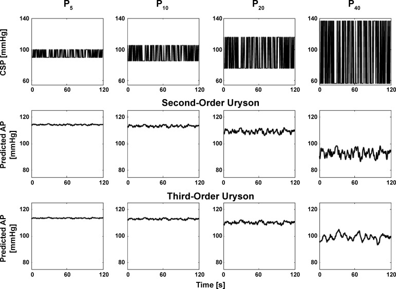
Abstract

The total baroreflex arc is the open-loop system relating carotid sinus pressure (CSP) to arterial pressure (AP). The nonlinear dynamics of this system were recently characterized. First, Gaussian white noise CSP stimulation was employed in open-loop conditions in normotensive and hypertensive rats with sectioned vagal and aortic depressor nerves. Nonparametric system identification was then applied to measured CSP and AP to establish a second-order nonlinear Uryson model. The aim in this study was to assess the importance of higher-order nonlinear dynamics via development and evaluation of a third-order nonlinear model of the total arc using the same experimental data. Third-order Volterra and Uryson models were developed by employing nonparametric and parametric identification methods. The R² values between the AP predicted by the best third-order Volterra model and measured AP in response to Gaussian white noise CSP not utilized in developing the model were 0.69 ± 0.03 and 0.70 ± 0.03 for normotensive and hypertensive rats, respectively. The analogous R² values for the best third-order Uryson model were 0.71 ± 0.03 and 0.73 ± 0.03. These R² values were not statistically different from the corresponding values for the previously established second-order Uryson model, which were both 0.71 ± 0.03 (P > 0.1). Furthermore, none of the third-order models predicted well-known nonlinear behaviors including thresholding and saturation better than the second-order Uryson model. Additional experiments suggested that the unexplained AP variance was partly due to higher brain center activity. In conclusion, the second-order Uryson model sufficed to represent the sympathetically mediated total arc under the employed experimental conditions.

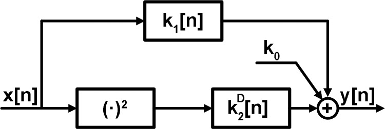
the total baroreflex arc has been defined as the open-loop system relating carotid sinus pressure (CSP) to arterial pressure (AP) (6). This system responds to fast CSP increases by decreasing AP and is an important contributor to cardiovascular regulation. Several investigators have characterized the system dynamics of the total arc in terms of a linear transfer function model (6, 8, 9, 12, 21). A few researchers have characterized the system dynamics in terms of a nonlinear model with an assumed structure (7, 11, 13). We recently characterized the system dynamics in terms of a nonlinear model that does not assume a particular structure for the nonlinearity (17, 18). We specifically applied Gaussian white noise CSP stimulation in an open-loop preparation and nonparametric system identification to develop a second-order Volterra model of the total arc for Wistar-Kyoto rats (WKY) and spontaneously hypertensive rats (SHR). We validated the nonlinear model by showing it could predict AP in response to Gaussian white noise CSP not utilized in developing the model significantly better than a linear model and well-known nonlinear behaviors including baroreflex thresholding and mean responses to input changes about the mean. We found that the structure of the nonlinear model was a linear dynamic system in parallel with a cascade combination of a squarer and a slower linear dynamic system, as shown in Fig. 1. Such an “Uryson” structure indicates that the square of the CSP input affects the AP output, whereas the CSP input at one time multiplied by the CSP input at another time has no impact on the AP output. We also found that the second-order nonlinear gain was enhanced in SHR relative to WKY, whereas the linear gain was preserved. This particular finding stressed the pitfall of ignoring total arc nonlinearity.

Fig. 1.

Previously established second-order nonlinear Uryson model of the total baroreflex arc (17, 18). x[n] is the carotid sinus pressure (CSP) input; y[n] is the arterial pressure (AP) output; and k₀,k₁[n], and $k_2^D\left[n\right]$ are the zeroth-, first-, and second-order system kernels.

A major assumption of our previous studies on total arc nonlinearity was that only second-order nonlinear dynamics were present. In this study, our aim was to assess the importance of higher-order nonlinear dynamics of the total arc to better understand nonlinear baroreflex functioning. To achieve this aim, we developed and evaluated third-order nonlinear dynamic models using the same experimental data. Our results indicate that a second-order Uryson model indeed sufficed to represent the total arc under the employed experimental conditions.

METHODS

Data collection and preprocessing.

Previously collected and preprocessed data were analyzed. These data are described in detail in several previous reports (9, 17, 18). Briefly, the data were from WKY and SHR with isolated carotid sinus regions (to open the baroreflex loop) and sectioned bilateral vagal and aortic depressor nerves (to eliminate other baroreflexes and thereby allow study of the sympathetically mediated carotid sinus baroreflex in isolation). The data included simultaneous CSP and AP measurements wherein CSP was stimulated with a Gaussian white noise signal with mean of 120 mmHg (normal CSP level of WKY) or 160 mmHg (normal CSP level of SHR), standard deviation of 20 mmHg, and a switching interval of 500 ms. There were 10 subject records from WKY at a mean CSP level of 120 mmHg, 7 subject records from SHR at the same mean level (SHR₁₂₀), and 5 subject records from SHR at a mean CSP level of 160 mmHg (SHR₁₆₀). Each subject record included a 6-min segment of stationary CSP and AP sampled at 2 Hz for developing the nonlinear models (training data) and a separate 3-min segment of such data for evaluating the models (testing data). The data also included additional CSP and AP measurements from the same subjects wherein CSP was stimulated using a staircase signal that started at 60 mmHg and then increased, step by step, in increments of 20 mmHg every 1 min up to at least 180 mmHg, for further evaluation of the models.

Nonlinear model and identification.

Any time-invariant system with fading memory can be represented with a Volterra series to within arbitrary precision (2). For a causal, discrete-time system, the Volterra model is given as follows:

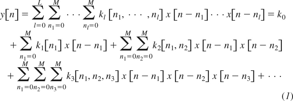Here, n is discrete-time, x[n] is the input, y[n] is the output, k_l[n₁,…,n_l] is the lth-order system kernel with memory M, and L is the order of nonlinearity. This model expands the present output sample in terms of the present and past input samples and products of an increasing number of present and past input samples. These input terms affect the output via the kernels.

In this general nonlinear model, the products of the input samples at both the same times (e.g., x²[n − 1], x³[n]) and different times (e.g., x[n − 2]x[n − 4]x[n − 1]x[n − 2]x[n − 3]) impact y[n]. Hence, the nonlinear kernels (second-order and higher) are functions of more than one variable representing the number of possible input times (e.g., the second-order kernel k₂[n₁,n₂] is a function of two variables, whereas the third-order kernel k₃[n₁, n₂, n₃] is a function of three variables). In an Uryson model (see second-order model in Fig. 1), which represents a class of simpler systems, the products of the input samples only at the same times (e.g., x²[n − 1], x³[n]) impact y[n]. Hence, the nonlinear kernels of an Uryson model are functions of one variable. Note that the Volterra model of Eq. 1 may be reduced to an Uryson model, if its nonlinear kernels are nonzero only when n₁ = n₂ = n₃ = …. In this case, the nonlinear kernels would be a function of one variable such that the products of input samples only at the same times would impact the output. Also note that n₁ = n₂ = n₃ = … is a line in multidimensional space and corresponds to the diagonal elements of the nonlinear kernels of the Volterra model. For example, k₂[n₁,n₂] may be visualized as a surface over a plane with axes n₁ and n₂. On this plane, n₁ = n₂ denotes the diagonal or identity line. For this reason, an Uryson model is equivalent to a Volterra model with only diagonal kernel elements. The kernels of an Uryson model are thus denoted with a superscript D henceforth ($k_2^D\left[n\right]$, $k_3^D\left[n\right]$).

In previous studies (17, 18), a second-order model (i.e., L = 2, which corresponds to the first three terms in Eq. 1) of the total arc was assumed. The second-order kernel was found to be diagonal (i.e., k₂[n₁,n₂] 0 for n₁ ≠ n₂) thereby indicating an Uryson structure. Furthermore, this kernel was not the same in shape as the first-order kernel (i.e., k₂[n₁,n₂] $=k_2^D\left[n\right]$, which is not proportional to k₁[n], for n₁ = n₂ = n), thereby indicating that the structure could not be further reduced.

In this study, the contribution of higher-order nonlinearity was explored by including the fourth term in Eq. 1 and thereby representing the total arc with the following third-order model (i.e., L = 3):

$$y\left[n\right]=k_0+{\displaystyle \sum }_{n_l=0}^M{k}_1\left[n_1\right]\hspace{0.17em}x\hspace{0.17em}\left[n-n_1\right]+{\displaystyle \sum }_{n_1=0}^M{k}_2^D\left[n_1\right]\hspace{0.17em}{x}^2\hspace{0.17em}\left[n-n_1\right]+{\displaystyle \sum }_{n_1=0}^M{\displaystyle \sum }_{n_2=0}^M{\displaystyle \sum }_{n_3=0}^M{k}_3\left[n_1,n_2,n_3\right]\hspace{0.17em}x\hspace{0.17em}\left[n-n_1\right]\hspace{0.17em}x\hspace{0.17em}\left[n-n_2\right]\hspace{0.17em}x\hspace{0.17em}\left[n-n_3\right]$$ (2)

Here, x[n] is the preprocessed CSP after removing its mean value, and y[n] is the preprocessed AP, whereas k₀, k₁[n], $k_2^D\left[n\right]$, and k₃[n₁, n₂, n₃] are the system kernels for estimation. The zeroth-order kernel k₀ is a constant that affects the mean value of y[n]. The first-order or linear kernel k₁[n], which is the time-domain version of the conventional transfer function, indicates how the present and past input samples (e.g., x[n] and x[n − 3]) affect the current output sample y[n]. The second-order kernel $k_2^D\left[n\right]$, which is Uryson in structure based on the previous work, indicates how the present and past squared input samples (e.g., x²[n] and x²[n − 2]) affect y[n]. Finally, the third-order kernel k₃[n₁, n₂, n₃] indicates how the product of three present and past input samples of same or different times affect y[n] (e.g, x[n − 1]x[n − 2]x[n − 3] is scaled by k₃[1,2,3] and x²[n]x[n − 3] is scaled by k₃[0,0,3] and then summed in the formation of y[n]). Note that this latter kernel is symmetric about its arguments (i.e., k₃[n₁, n₂, n₃] = k₃[n₁, n₃, n₂] = k₃[n₂, n₁, n₃] = k₃[n₂, n₃, n₁] = k₃[n₃, n₁, n₂] = k₃[n₃, n₂, n₁]).

The kernels of higher-order Volterra models are difficult to estimate directly, so an orthogonal representation of Eq. 2 for Gaussian inputs was employed to facilitate the estimation (see appendix a). This representation allowed the kernels to be estimated separately. Note that separate estimation of individual kernels makes the estimation straightforward compared with simultaneous estimation of all kernels. Also note that since the estimation of one kernel has little impact on the estimation of other kernels, the previous finding that the second-order kernel was diagonal could be employed in the model of Eq. 2 without affecting the third-order kernel estimates herein. A sequential estimation process was specifically applied (see appendices b and c). In particular, each kernel was estimated, one at a time and in order, using the measured x[n] and y[n] after subtracting the contribution of all previous kernel estimates from y[n]. Several kernel estimation methods were applied including the frequency-domain method for Gaussian inputs (5) and cross-correlation method for Gaussian white noise inputs (15). The third-order kernel estimates were then examined to arrive at reduced nonlinear models (see results). The reduced models were reestimated to yield potentially more predictive models. Several kernel estimation methods were again applied including the frequency-domain method for Gaussian inputs, Laguerre expansion method for Gaussian and arbitrary inputs (15, 22), and cross-correlation method for Gaussian white noise inputs. See estimates herein. A sequential estimation process was specifically applied (see appendices for the details of the most successful estimation methods and discussion for commentary on the various methods). In all cases, the kernel memory M was set to 25 s based on previous studies (17, 18).

Model evaluation.

The resulting third-order nonlinear models were evaluated in terms of their capacity to predict AP in response to three different CSP inputs. First, the CSP inputs from the Gaussian white noise testing data were applied to the individual subject models and the R² values between the predicted and measured AP outputs were computed. These R² values and the previously reported R² values for the second-order Uryson and linear models (17, 18) were then compared after log transformation via paired t-tests with Holm’s correction for multiple comparisons (4). For completeness, this process was also employed for the Gaussian white noise training data to gauge model fitting, rather than more important model predictive, abilities. Second, the staircase CSP input specified above was applied to the individual subject models, and the resulting steady-state AP outputs were plotted against the corresponding CSP levels. These predicted static nonlinearity curves were then qualitatively compared with the measured curves and the previously reported curves predicted by the second-order Uryson model. Third, binary white noise CSP with mean of 95 mmHg, amplitudes ± 5, ± 10, ± 20, and ± 40 mmHg, and switching interval of 500 ms were applied to the group average models. The predicted AP responses were then qualitatively compared with the previously reported responses predicted by the second-order Uryson model. While reference AP measurements in response to binary white noise of increasing amplitude were not available in the subjects studied herein, the second-order Uryson model was previously shown to correctly predict mean AP reductions with increasing CSP amplitude (17).

RESULTS

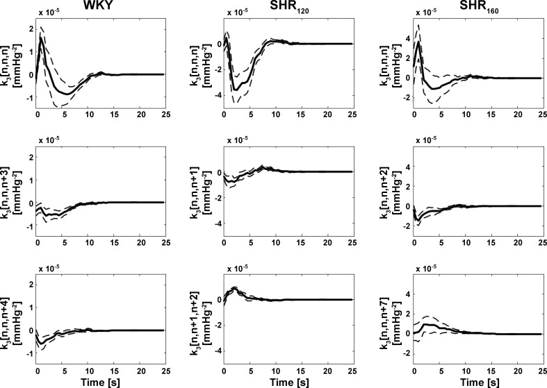
Similar to previous reports (17, 18), the frequency-domain method for Gaussian inputs (see appendix b) yielded the smoothest estimates of the kernels in the total arc model of Eq. 2. The newly estimated third-order kernels are four-dimensional and cannot be visualized. So, each two-dimensional slice of these kernels was examined. A two-dimensional slice of a third-order kernel is mathematically defined as k₃[n,n + a,n+b], where a and b are fixed values between 0 and M (the kernel memory) inclusive. Because of the symmetry of the third-order kernel mentioned above, all slices over the a and b range collectively make up the kernel. As can be inferred from Eq. 2, a slice carries meaning in the sense that it is convolved with a cubic input term in the formation of the output. Figure 2 shows the three slices of the group average (mean with standard errors over the subjects) third-order kernel estimates with the largest energies for WKY, SHR₁₂₀, and SHR₁₆₀. Energy is defined here as the sum of squares of the samples of a kernel slice. The diagonal slices (k₃[n,n,n]) clearly exhibited the largest energies on average. Figure 3 shows the energy of each group average two-dimensional slice, normalized by the diagonal slice energy, in descending order of value for WKY, SHR₁₂₀, and SHR₁₆₀. For comparison, this figure includes the analogous results for the second-order Volterra kernel estimates from previous reports (17, 18). The normalized energies of the third-order kernels were smaller than unity both in a statistical sense (P value typically <0.01 via one sample t-tests) and a magnitude sense, especially for SHR₁₂₀. Hence, the third-order kernel was virtually diagonal for SHR₁₂₀ (similar to all second-order kernels) and approximately diagonal for WKY and SHR₁₆₀. As a result, the model of Eq. 2 was reduced to the following third-order Uryson model:

$$y\left[n\right]=k_0+{\displaystyle \sum }_{n_l=0}^M{k}_1\left[n_1\right]x\hspace{0.17em}\left[n-n_1\right]+{\displaystyle \sum }_{n_1=0}^M{k}_2^D\left[n_1\right]x^2\left[n-n_1\right]+{\displaystyle \sum }_{n_1=0}^M{k}_3^D\left[n_1\right]x^3\left[n-n_1\right]$$ (3)

Fig. 2.

Group average two-dimensional (2D) slices of the estimated (four-dimensional) third-order kernels (k₃[n₁,n₂,n₃]) in Eq. 2 with the largest (top), second largest (middle), and third largest (bottom) energies. The group averages are illustrated as the mean over the subjects (solid line) and mean ± SE over the subjects (dashed line), whereas energy is defined as the sum of squares of the samples of the kernel slice. The diagonal slice (k₃[n,n,n]) was largest in energy for Wistar-Kyoto (WKY rats during Gaussian white noise CSP stimulation with mean of 120 mmHg), spontaneously hypertensive rats (SHR₁₂₀ during the same CSP stimulation), and SHR₁₆₀ (during the Gaussian white noise CSP stimulation but with mean of 160 mmHg).

Fig. 3.

Energy of each group average 2D slice of the estimated second-order Volterra kernels from Refs. 17 and 18 and third-order kernels, normalized by the diagonal slice energy, in descending order of value for WKY, SHR₁₂₀, and SHR₁₆₀. The second-order kernel was always diagonal, whereas the third-order kernel was virtually diagonal for SHR₁₂₀ and approximately diagonal for WKY and SHR₁₆₀.

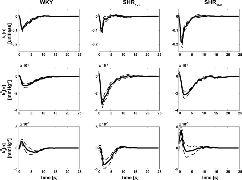
The kernels in this model were reestimated. The frequency-domain method and more parsimonious Laguerre method for Gaussian inputs (see appendix c) yielded the visually smoothest kernel estimates. Figure 4 shows the group average kernel estimates of the former method only, as the estimates of the latter method were similar. The first- and second-order kernel estimates in this figure were reported previously (17, 18). The newly estimated third-order kernels did not appear proportional to the first- and second-order kernels, thereby suggesting that the model cannot be further reduced to a Hammerstein model (19) in general. The third-order kernel estimates appeared qualitatively similar for WKY and SHR₁₆₀ but different for SHR₁₂₀. The former two kernels showed a positive, open-loop contribution to AP regulation (i.e., an increase in CSP would increase AP), whereas the latter kernel showed a negative, open-loop contribution (i.e., an increase in CSP would decrease AP). However, the overall contribution of the three kernels was of negative, open-loop character for WKY, SHR₁₂₀, and SHR₁₆₀. The Laguerre expansion method for Gaussian inputs represented the third-order Uryson model with 19 parameters on average (6 parameters for each of the three kernels plus 1 smoothing parameter; see appendix c), whereas the frequency-domain method for Gaussian inputs represented the Uryson model with 50 parameters per kernel (M = 25 s times 2 Hz sampling rate; see Eq. 3).

Fig. 4.

Group average first-, second-, and third-order kernel estimates of reduced Uryson models of the total arc for WKY, SHR₁₂₀, and SHR₁₆₀ via the frequency-domain method for Gaussian inputs. The group averages are again illustrated as the mean over the subjects (solid line) and mean ± SE over the subjects (dashed line). The three kernel estimates via the Laguerre expansion method for Gaussian inputs were similar and thus not shown. The three kernels were not proportional to each other, thereby indicating that the model could not be further reduced.

Table 1 shows the group average R² values between the AP predicted by the individual subject third-order nonlinear models and the measured AP when stimulated by Gaussian white noise CSP in the training and testing data. Table 1 also includes the corresponding, previously reported results for the second-order Uryson and linear models (17, 18). When compared with the second-order Uryson model, the third-order model of Eq. 2 improved the R² value for the training data (by 14–27%) but not the testing data. Hence, the third-order model was not better than the second-order model in terms of AP prediction. Note that appreciable improvement in model performance in training data but not testing data also implies that the model was overfitted. The third-order Uryson model of Eq. 3 also did not improve upon the R² value, thereby likewise indicating that it was not better than the second-order Uryson model. Furthermore, the R² value between the AP predicted by each of the third-order models and the second-order Uryson model in the Gaussian white noise testing data was typically >0.95. Hence, the third-order models actually yielded very similar AP predictions to the second-order Uryson model in these data.

Table 1.

Group average R² values between AP predicted by models of the total baroreflex arc and measured AP

	Linear	Second-Order Uryson	Third-Order Volterra	Third-Order Uryson (Frequency-Domain)	Third-Order Uryson (Laguerre Expansion)
WKY
Training data	0.73 ± 0.03	0.79 ± 0.03*	0.90 ± 0.01*†	0.80 ± 0.03*†	0.80 ± 0.03*†
Testing data	0.64 ± 0.03	0.71 ± 0.03*	0.69 ± 0.03*†	0.71 ± 0.03*	0.71 ± 0.03*
SHR120
Training data	0.53 ± 0.05	0.69 ± 0.04*	0.88 ± 0.01*†	0.72 ± 0.05*†	0.71 ± 0.04*†
Testing data	0.45 ± 0.03	0.64 ± 0.03*	0.64 ± 0.04*	0.65 ± 0.04*	0.66 ± 0.04*
SHR160
Training data	0.63 ± 0.05	0.71 ± 0.05*	0.88 ± 0.03*†	0.72 ± 0.05*	0.72 ± 0.05*
Testing data	0.59 ± 0.04	0.71 ± 0.03*	0.70 ± 0.03*	0.73 ± 0.03*	0.72 ± 0.03*

Values are means ± SE. Third-order Volterra model refers to Eq. 2. AP, arterial pressure; WKY, Wistar-Kyoto rats during Gaussian white noise carotid sinus pressure (CSP) stimulation with mean of 120 mmHg; SHR₁₂₀ and SHR₁₆₀, spontaneously hypertensive rats during the same CSP stimulation with mean of 120 and 160 mmHg, respectively. * and †Statistical significance for paired t-test comparison (after Holm’s correction for three comparisons) with corresponding linear model and second-order Uryson model, respectively.

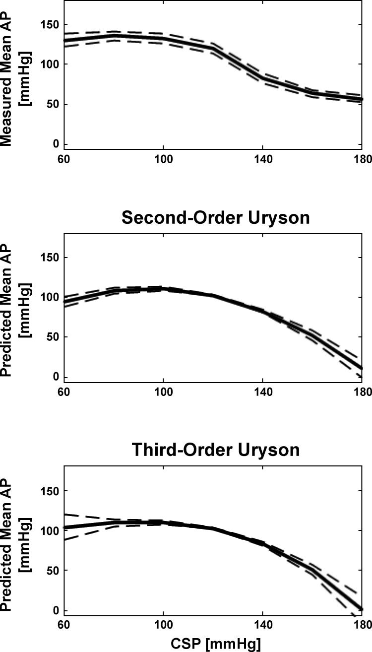
Figure 5 shows the group average static nonlinearity curves measured and predicted by the third-order Uryson model (identified via the frequency-domain method for Gaussian inputs) as well as the second-order Uryson model for WKY. Figure 6 shows the AP predicted by the two Uryson models in response to binary white noise CSP of increasing amplitude for WKY. The third-order model again yielded similar AP predictions to the second-order model. This finding also held for the third-order model of Eq. 2 and SHR₁₂₀ and SHR₁₆₀ (results not shown for convenience). Hence, the third-order nonlinear models also did not predict baroreflex thresholding and saturation and mean responses to input changes about the mean better than the second-order Uryson model.

Fig. 5.

Group average static nonlinearity curves measured and predicted by the second- and third-order Uryson models of the total arc (identified via the frequency-domain method for Gaussian inputs) in response to a staircase CSP input for WKY. The two models similarly predicted thresholding (maximal AP response) but not saturation (minimal AP response).

Fig. 6.

AP predicted by the group average second- and third-order Uryson models of the total arc (identified via the frequency-domain method for Gaussian inputs) in response to binary white noise of increasing amplitude for WKY. The two models similarly predicted reductions in mean AP in response to CSP changes about the mean.

DISCUSSION

This study represents part three of a series of studies on nonlinear identification of the total baroreflex arc–the sympathetically mediated carotid sinus baroreflex relating CSP to AP in open-loop conditions. In parts one and two (17, 18), we applied Gaussian white noise CSP stimulation and nonparametric system identification to measured CSP and AP to establish a second-order Uryson model (i.e., a Volterra model with diagonal kernels) of the total arc for WKY and SHR (see Fig. 1). However, a major assumption therein was that only second-order nonlinear dynamics were important. In part three herein, to better understand nonlinear baroreflex functioning, we investigated the contribution of higher-order nonlinearity by developing a third-order nonlinear model using the same data for analysis.

We used a third-order Volterra model but with a second-order Uryson kernel (see Eq. 2). We estimated the first- and second-order kernels using the frequency-domain method for Gaussian inputs (see appendices a and b), which we previously found to yield the smoothest kernels (17, 18). Since estimation of higher-order kernels from short data periods (6 min) is challenging, we applied several identification methods to estimate the third-order kernels. The nonparametric identification methods, which do not assume a particular kernel form, included the frequency-domain method for Gaussian inputs (see appendix b) and cross-correlation method (15), which assumes the input is Gaussian and white. We again found that the frequency-domain method for Gaussian inputs was most effective, as the CSP input was not strictly white due to the finite data periods. The resulting third-order kernel estimates revealed an Uryson structure for SHR₁₂₀ (SHR with Gaussian white noise stimulation at the normal CSP level for WKY) and an approximate Uryson structure for WKY and SHR₁₆₀ (SHR with the same stimulation but at the prevailing CSP level for SHR) (see Figs. 2 and 3). It is possible that the diagonal nature of the third-order kernels for WKY and SHR₁₆₀ was partially masked by noise arising from the identification of higher-order kernels from short data periods in the presence of stronger linearity (see Table 1). Furthermore, since the second-order kernel, which is easier to estimate, is surely Uryson (see Fig. 3), the third-order kernel may indeed likewise show such structure. At the same time, we acknowledge the possibility of nontrivial error in the third-order kernel estimates. Parametric identification methods could possibly improve kernel estimation from short data periods by reducing the number of estimated parameters via assumption of a particular kernel form. We also applied such methods including popular Laguerre expansion methods (15). However, these methods artificially smoothed the kernels so as to obfuscate a diagonal appearance.

We therefore moved to a reduced, third-order Uryson model (see Eq. 3). We again applied various identification methods to reestimate the kernels of this model with potentially greater accuracy. The methods included the frequency-domain method for Gaussian inputs, cross-correlation method, and Laguerre expansion methods for Gaussian and arbitrary inputs. We found that the frequency-domain method and Laguerre expansion method for Gaussian inputs (see appendix c) yielded the smoothest estimates, as the input was not strictly white and the requisite computation of higher-order correlations was more robust by leveraging the Gaussian nature of the inputs. The resulting kernel estimates of the two methods were similar. The third-order kernel estimates were not proportional to the first- and second-order kernel estimates (see Fig. 4), thereby indicating that the third-order model could not be further reduced. The Laguerre expansion method for Gaussian inputs used only about one-fifth of the parameters to represent the third-order Uryson model as the frequency-domain method for Gaussian inputs used to represent the second-order Uryson model. Hence, the third-order Uryson model was likely well estimated.

Neither the third-order Uryson model nor the complete third-order nonlinear model of Eq. 2 predicted AP in response to Gaussian white noise CSP in the testing data better than the previously established second-order Uryson model (see Table 1). In fact, the AP predictions of the third-order models and second-order Uryson model were very similar in these data. Furthermore, both of the third-order models could not offer added value in predicting well-known nonlinear behaviors including baroreflex thresholding and saturation and mean responses to input changes about the mean over the second-order Uryson model (see Figs. 5 and 6). Since there is a possibility that the third-order kernel was actually not Uryson, we formed a set of third-order kernels using the highest energy slices of the third-order Volterra kernel estimate (see Fig. 3). Such kernels are more complicated than the Uryson kernel but simpler than the Volterra kernel. However, the third-order models with these kernel estimates also did not improve the AP prediction in any way (results not shown). Hence, even though the third-order kernels were not merely noise (see Fig. 4), they may be interpreted as small in the sense of contributing relatively little to AP prediction. Note that, as mentioned above, a nonlinear model including only the first- and third-order kernels would not have performed better due to orthogonality arising from use of Gaussian inputs. Also note that while fourth-order and even higher-order kernels could possibly contribute to AP prediction, since the first-order kernel, which is odd, and the second-order kernel, which is even, both contributed significantly, we doubt that kernels of order exceeding three would be important here.

Higher-order nonlinearity therefore does not appear to be a contributing factor to the unexplained AP variance of ~30% during the Gaussian white noise CSP stimulation in the testing data (see Table 1), as we had previously hypothesized (17). These variations, which were not white (results not shown), could instead be due to nonstationarity of the CSP and AP data, sympathetic nerve activity (SNA) from higher brain centers, and other fast-acting regulatory mechanisms. Note that measurement noise may not be a contributing factor, as the data were invasively measured and then low-pass filtered and down sampled all the way to 2 Hz.

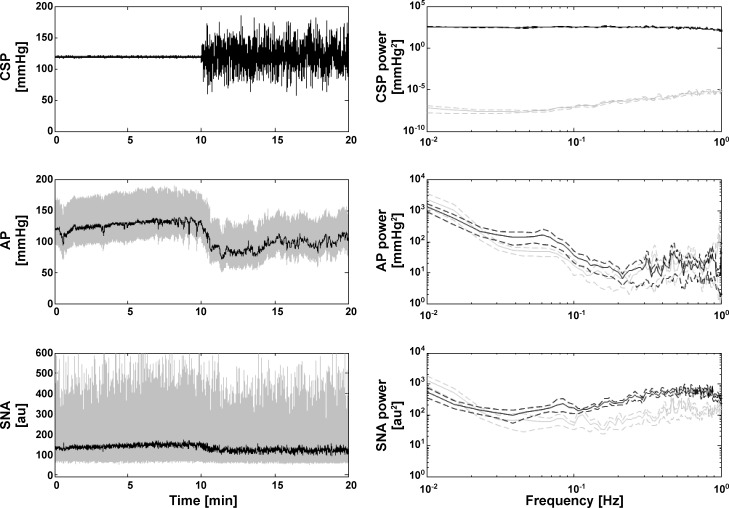
To shed further light on the sources of the unexplained AP variance, we performed preliminary experiments in six WKY with CSP fixed to 120 mmHg followed by Gaussian white noise CSP stimulation. Figure 7 shows the measured CSP, AP, and SNA for one subject along with the corresponding group average power spectra. The spectral powers in AP and SNA within ~0.04 Hz were not reduced during fixed CSP relative to Gaussian white noise CSP. These results suggest that SNA from higher brain centers indeed contributed to the unexplained AP variance, particularly in the low frequency regime. Note that turning the CSP input “off” changed the mean AP and thus the system operating point. Hence, the AP variability at fixed CSP and the unexplained AP variability of the nonlinear models may not be comparable. Also note that the SNA from higher brain centers and any data nonstationarity surely introduced error in the kernel estimates herein and perhaps the precision error in the low frequency regime in particular.

Fig. 7.

Representative time series for AP and sympathetic nerve activity [SNA; measured from splanchnic nerve and then normalized as described elsewhere (17)] in response to fixed and Gaussian white noise CSP stimulations for one WKY (left). au, arbitrary units. Group average power spectra for CSP, AP, and SNA (right). Gray and black lines indicate the fixed and Gaussian white noise CSP inputs, respectively. These preliminary results indicate that SNA from higher brain centers contribute to the unexplained AP variance of the nonlinear total arc models (see Table 1), particularly in the low frequency regime.

We conclude that a second-order Uryson model of the total arc surely s uffices compared with a third-order Uryson model and may likely suffice compared with higher-order nonlinear models in general. This conclusion is only valid over the range of CSP and AP data utilized to develop the models. This range did not include CSP levels to elicit both thresholding (maximum AP response) and saturation (minimum AP response), which are nonlinear baroreflex behaviors that have been repeatedly observed (3, 10, 16). In particular, the range did not excite the baroreflex saturation regime [which starts at ~160 mmHg for WKY and ~200 mmHg for SHR (20)]. As a result, the nonlinear models could only predict baroreflex thresholding (see Fig. 5). However, baroreflex thresholding and saturation together exhibit an odd symmetry about the nominal CSP set point (e.g., they could be modeled with a sigmoid function) and therefore would require odd-order nonlinearity for its representation (15). Hence, a nonlinear model of order exceeding two should be needed to represent the total arc over the entire CSP input range. In sum, this third part of a series of studies on nonlinear identification of the total arc justified the earlier assumption of second-order nonlinearity under the employed experimental conditions.

Perspectives and Significance

It is well known that the carotid sinus baroreflex displays nonlinear dynamic behaviors. Even so, many studies in the past have assumed that it acts as a linear system. We previously employed Gaussian white noise CSP stimulation in open-loop conditions and nonparametric system identification to establish a second-order nonlinear model of the sympathetically mediated carotid sinus baroreflex (17, 18). We validated the model by showing that it could predict AP significantly better than a standard linear model in response to Gaussian white noise CSP not utilized in developing the model as well as important nonlinear behaviors including thresholding and mean responses to input changes about the mean. The model revealed the “Uryson” structure of the second-order nonlinearity of the total arc and showed that its second-order nonlinear gain is selectively enhanced in a chronic hypertension setting. Here, we buttressed the major previous assumption that the baroreflex nonlinearity did not extend beyond second-order under the employed experimental conditions. Future studies are needed to: 1) elucidate baroreflex nonlinearity over a wider system operating range than that attained by the experimental conditions; herein 2); investigate baroreflex nonlinearity in closed-loop conditions [via parametric identification (25) and the established second-order Uryson model]; and 3) discover the mechanism of baroreflex nonlinearity [which may be related to the slow, afferent C-fiber pathway (23, 24)] including the unexplained AP variations. Such future nonlinear modeling endeavors may enhance our understanding of the baroreflex in health and disease. The established nonlinear baroreflex models could also conceivably be used to help improve baroreflex stimulation strategies for treating central baroreflex failure and drug-resistant hypertension (10).

GRANTS

This work was supported in part by the National Institutes of Health Grant EB018818.

DISCLOSURES

No conflicts of interest, financial or otherwise, are declared by the author(s).

AUTHOR CONTRIBUTIONS

M.M., K.S., and R.M. conception and design of research; M.M. analyzed data; M.M., T.K., K.S., M.S., and R.M. interpreted results of experiments; M.M. and T.K. prepared figures; M.M. and R.M. drafted manuscript; M.M., T.K., K.S., M.S., and R.M. approved final version of manuscript; T.K. performed experiments; T.K., K.S., and M.S. edited and revised manuscript.

APPENDIX A

To facilitate system identification, the following orthogonal representation of the third-order nonlinear model of Eq. 2 for Gaussian inputs (1, 14) was employed:

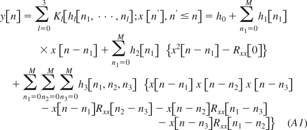Here, K_l[·] is the lth-order functional; h₀, h₁[n], h₂[n], and h₃[n₁,n₂,n₃] are system kernels, which are symmetric with respect to their arguments; and R_xx(n) is the autocorrelation function of the zero-mean Gaussian input x[n]. Since the functionals are orthogonal to each other, the kernels of this equation may be estimated sequentially (see appendices b and c). The Volterra kernels in Eq. 2 may then be computed from the estimated quantities and R_xx(n) as follows:

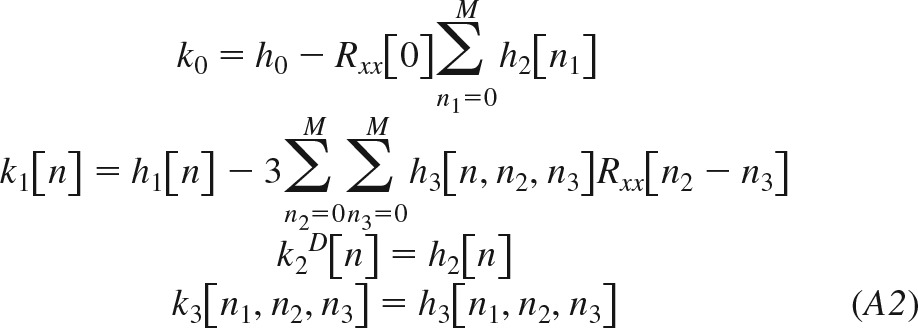APPENDIX B

The kernels h₀, h₁[n], h₂[n], and h₃[n₁,n₂,n₃], and in Eq. A1 were estimated from x[n] after removing its mean value and y[n] using the frequency-domain method for Gaussian inputs. This method, which minimizes the mean-squared output prediction error and yielded relatively smooth kernel estimates, is described in detail elsewhere (5). Briefly, the kernels were estimated in succession according to the following four steps:

Step 1:

$$h_0=E\left(y\left[n\right]\right)$$

where E(·) is the expectation operator.

Step 2:

$$y_1\left[n\right]=y\left[n\right]-h_0$$

$$H_1\left(f\right)=\mathcal{F}\left\{h_1\left[n\right]\right\}=\frac{\mathcal{F}\left\{R_{y_{1}x}\left[n\right]\right\}}{\mathcal{F}\left\{R_{xx}\left[n\right]\right\}}$$

where R(·) is the auto- or cross-correlation function between the indicated signals, and $\mathcal{F}(\cdot )$ is the standard Fourier Transform operator.

Step 3:

$$y_2\left[n\right]=y_1\left[n\right]-{\displaystyle \sum }_{n_1=0}^M{h}_1\left[n_1\right]\hspace{0.17em}x\left[n-n_1\right]$$

$$x_2\left[n\right]=x^2\left[n\right]$$

$$H_2\left(f\right)=\mathcal{F}\left\{h_2\left[n\right]\right\}=\frac{\mathcal{F}\left\{R_{y_2{x}_2}\left[n\right]\right\}}{\mathcal{F}\left\{2R^2{}_{xx}\left[n\right]\right\}}$$

Step 4:

$$y_3\left[n\right]=y_2\left[n\right]-{\displaystyle \sum }_{n_1=0}^M{h}_2\left[n_1\right]\hspace{0.17em}\left\{x^2\left[n-n_1\right]-R_{xx}\left[0\right]\right\}$$

$$H_3\left(f_1,f_2,f_3\right)\}={\mathcal{F}}_3\left\{h_3\left[n_1,n_2,n_3\right]\right\}=\frac{1}{6}\left\{\frac{{\mathcal{F}}_3\left\{R_{y_{3}xxx}[n_1,n_2,n_3]\right\}}{\mathcal{F}\left\{R_{xx}\left[n_1\right]\right\} \mathcal{F}\left\{R_{xx}\left[n_2\right]\right\} \mathcal{F}\left\{R_{xx}\left[n_3\right]\right\}}\right\}$$

where ${\mathcal{F}}_3(\cdot )$ is the three-dimensional Fourier Transform operator. Note that E(·) and R(·) above were computed via the standard sample mean and unbiased correlation function estimates.

APPENDIX C

An orthogonal representation of the third-order Uryson model of Eq. 3 for Gaussian inputs was likewise employed. The equations are the same as in appendix a but with the following two adjustments:

$$K_3\left[h_3\left[n\right];x\left[n^{\prime }\right],n^{\prime }\le n\right]={\displaystyle \sum }_{n_1}{h}_3\left[n_1\right]x^3\left[n-n_1\right]-3R_{xx}\left[0\right]{\displaystyle \sum }_{n_1}{h}_3\left[n_1\right]\hspace{0.17em}\hspace{0.17em}x\hspace{0.17em}\left[n-n_1\right]$$

$$k_1\left[n\right]=h_1\left[n\right]-3h_3\left[n\right]\hspace{0.17em}{R}_{xx}\left[0\right]$$

The kernels h₀, h₁[n], h₂[n], and h₃[n] were again estimated from x[n] after removing its mean value and y[n] using the frequency-domain method for Gaussian inputs. This method yielded relatively smooth kernel estimates. The kernels were estimated in succession according to the first three steps in appendix b and then the following fourth step:

$$y_3\left[n\right]=y_2\left[n\right]-{\displaystyle \sum }_{n_1=0}^M{h}_2\hspace{0.17em}\left[n_1\right]\hspace{0.17em}\left\{x^2\left[n-n_1\right]-R_{xx}\left[0\right]\right\}$$

$$x_3\left[n\right]=x^3\left[n\right]$$

$$H_3\left(f\right)=\mathcal{F}\left\{h_3\left[n\right]\right\}=\frac{\mathcal{F}\left\{R_{y_3{x}_3}\left[n\right]\right\}}{6\mathcal{F}\left\{R^3{}_{xx}\left[n\right]\right\}}$$

The four kernels were also estimated from the same data using the Laguerre expansion method for Gaussian inputs (15). This more parsimonious method produced similar kernel estimates. More specifically, the first-, second-, and third-order kernels were assumed to be represented by a linear combination of B Laguerre basis functions as follows:

$$h_i\left[n\right]={\displaystyle \sum }_{j=1}^B{a}_{ij}{b}_j\hspace{0.17em}\left[n\right],\hspace{0.17em}i=1,2,3$$

Here, a_if is the jth coefficient of the ith-order kernel for estimation, and b_j[n] is the jth Laguerre basis function. This function is given as follows:

$$b_j\hspace{0.17em}\left[n\right]={\text{α}}^{\left(n_1-j\right)/2}{\left(1-\text{α}\right)}^{1/2}{\displaystyle \sum }_{k=0}^j{\left(-1\right)}^k\left(\begin{array}{c}n\\ k\end{array}\right)\left(\begin{array}{c}j\\ k\end{array}\right){\text{α}}^{j-k}{\left(1-\text{α}\right)}^k$$

where α (0 < α < 1) is a smoothing parameter that determines the rate of exponential decay of the Laguerre function. The coefficients of each kernel were estimated in succession by minimizing the mean-squared output prediction error. That is, for fixed B and α values, the B coe;fficients for each kernel were estimated via solution of the following B×B linear system of normal equations:

$${\displaystyle \sum }_{k^{\prime }}{b}_{j_0}\hspace{0.17em}\left[k^{\prime }\right]R_{x^i{y}_i}\left[k^{\prime }\right]=\left(i!\right){\displaystyle \sum }_{j=1}^B{a}_{ij}{\displaystyle \sum }_k{\displaystyle \sum }_{k^{\prime }}{b}_j\left[k\right]b_{j_0}\left[k^{\prime }\right]R^i{}_{xx}\left[k-{k^{\prime }}^{}\right]\hspace{0.17em}\mathrm{f}\mathrm{o}\mathrm{r}\hspace{0.17em}{j}_0=1,\cdots ,B$$

where R(·) is the auto- or cross-correlation function between the indicated signals, and y_i is the output after subtracting the contribution of all previously estimated kernel (see appendix b). To determine B and α , the same α value was assumed for all kernels, and the B value was assumed to be between 1 and 10. For a fixed α value, the value of B was determined for each kernel by finding the value for which the mean-squared output prediction error no longer significantly decreased. This calculation was repeated for each α value between 0 and 1, and the value that minimized the mean-squared output prediction error was selected.

REFERENCES

- 1.Barrett JF. The use of functionals in the analysis of non-linear physical systems. J Electron Contr 15: 567–615, 1963. doi: 10.1080/00207216308937611. [DOI] [Google Scholar]
- 2.Boyd S, Chua L. Fading memory and the problem of approximating nonlinear operators with Volterra series. IEEE Trans Circ Syst 32: 1150–1161, 1985. doi: 10.1109/TCS.1985.1085649. [DOI] [Google Scholar]
- 3.Chen HI, Bishop VS. Baroreflex open-loop gain and arterial pressure compensation in hemorrhagic hypotension. Am J Physiol Heart Circ Physiol 245: H54–H59, 1983. [DOI] [PubMed] [Google Scholar]
- 4.Holm S. A simple sequentially rejective multiple test procedure. Scand J Stat 6: 66–70, 1979. [Google Scholar]
- 5.Hong JY, Kim YC, Powers EJ. On modeling the nonlinear relationship between fluctuations with nonlinear transfer functions. Proc IEEE 68: 1026–1027, 1980. doi: 10.1109/PROC.1980.11786. [DOI] [Google Scholar]
- 6.Ikeda Y, Kawada T, Sugimachi M, Kawaguchi O, Shishido T, Sato T, Miyano H, Matsuura W, Alexander J Jr, Sunagawa K. Neural arc of baroreflex optimizes dynamic pressure regulation in achieving both stability and quickness. Am J Physiol Heart Circ Physiol 271: H882–H890, 1996. [DOI] [PubMed] [Google Scholar]
- 7.Kawada T, Li M, Kamiya A, Shimizu S, Uemura K, Yamamoto H, Sugimachi M. Open-loop dynamic and static characteristics of the carotid sinus baroreflex in rats with chronic heart failure after myocardial infarction. J Physiol Sci 60: 283–298, 2010. doi: 10.1007/s12576-010-0096-9. [DOI] [PMC free article] [PubMed] [Google Scholar]
- 8.Kawada T, Sato T, Inagaki M, Shishido T, Tatewaki T, Yanagiya Y, Zheng C, Sugimachi M, Sunagawa K. Closed-loop identification of carotid sinus baroreflex transfer characteristics using electrical stimulation. Jpn J Physiol 50: 371–380, 2000. doi: 10.2170/jjphysiol.50.371. [DOI] [PubMed] [Google Scholar]
- 9.Kawada T, Shimizu S, Kamiya A, Sata Y, Uemura K, Sugimachi M. Dynamic characteristics of baroreflex neural and peripheral arcs are preserved in spontaneously hypertensive rats. Am J Physiol Regul Integr Comp Physiol 300: R155–R165, 2011. doi: 10.1152/ajpregu.00540.2010. [DOI] [PubMed] [Google Scholar]
- 10.Kawada T, Sugimachi M. Open-loop static and dynamic characteristics of the arterial baroreflex system in rabbits and rats. J Physiol Sci 66: 15–41, 2016. doi: 10.1007/s12576-015-0412-5. [DOI] [PMC free article] [PubMed] [Google Scholar]
- 11.Kawada T, Yanagiya Y, Uemura K, Miyamoto T, Zheng C, Li M, Sugimachi M, Sunagawa K. Input-size dependence of the baroreflex neural arc transfer characteristics. Am J Physiol Heart Circ Physiol 284: H404–H415, 2003. doi: 10.1152/ajpheart.00319.2002. [DOI] [PubMed] [Google Scholar]
- 12.Kubo T, Imaizumi T, Harasawa Y, Ando S, Tagawa T, Endo T, Shiramoto M, Takeshita A. Transfer function analysis of central arc of aortic baroreceptor reflex in rabbits. Am J Physiol Heart Circ Physiol 270: H1054–H1062, 1996. [DOI] [PubMed] [Google Scholar]
- 13.Levison WH, Barnett GO, Jackson WD. Nonlinear analysis of the baroreceptor reflex system. Circ Res 18: 673–682, 1966. doi: 10.1161/01.RES.18.6.673. [DOI] [PubMed] [Google Scholar]
- 14.Marmarelis PZ, Marmarelis VZ. Analysis of Physiological Systems: The White-Noise Approach. New York: Plenum; 1978. doi: 10.1007/978-1-4613-3970-0 [DOI] [Google Scholar]
- 15.Marmarelis VZ. Nonlinear Dynamic Modeling of Physiological Systems. Wiley, 2004. doi: 10.1002/9780471679370 [DOI] [Google Scholar]
- 16.McDowall LM, Dampney RAL. Calculation of threshold and saturation points of sigmoidal baroreflex function curves. Am J Physiol Heart Circ Physiol 291: H2003–H2007, 2006. doi: 10.1152/ajpheart.00219.2006. [DOI] [PubMed] [Google Scholar]
- 17.Moslehpour M, Kawada T, Sunagawa K, Sugimachi M, Mukkamala R. Nonlinear identification of the total baroreflex arc. Am J Physiol Regul Integr Comp Physiol 309: R1479–R1489, 2015. doi: 10.1152/ajpregu.00278.2015. [DOI] [PMC free article] [PubMed] [Google Scholar]
- 18.Moslehpour M, Kawada T, Sunagawa K, Sugimachi M, Mukkamala R. Nonlinear identification of the total baroreflex arc: chronic hypertension model. Am J Physiol Regul Integr Comp Physiol 310: R819–R827, 2016. doi: 10.1152/ajpregu.00424.2015. [DOI] [PMC free article] [PubMed] [Google Scholar]
- 19.Rébillat M, Hennequin R, Corteel É, Katz BFG. Identification of cascade of Hammerstein models for the description of nonlinearities in vibrating devices. J Sound Vibrat 330: 1018–1038, 2011. doi: 10.1016/j.jsv.2010.09.012. [DOI] [Google Scholar]
- 20.Sata Y, Kawada T, Shimizu S, Kamiya A, Akiyama T, Sugimachi M. Predominant role of neural arc in sympathetic baroreflex resetting of spontaneously hypertensive rats. Circ J 79: 592–599, 2015. doi: 10.1253/circj.CJ-14-1013. [DOI] [PubMed] [Google Scholar]
- 21.Sato T, Kawada T, Inagaki M, Shishido T, Sugimachi M, Sunagawa K. Dynamics of sympathetic baroreflex control of arterial pressure in rats. Am J Physiol Regul Integr Comp Physiol 285: R262–R270, 2003. doi: 10.1152/ajpregu.00692.2001. [DOI] [PubMed] [Google Scholar]
- 22.Schetzen M. The Volterra and Wiener Theories of Nonlinear Systems. Wiley, 1980. [Google Scholar]
- 23.Seagard JL, Hopp FA, Drummond HA, Van Wynsberghe DM. Selective contribution of two types of carotid sinus baroreceptors to the control of blood pressure. Circ Res 72: 1011–1022, 1993. doi: 10.1161/01.RES.72.5.1011. [DOI] [PubMed] [Google Scholar]
- 24.Thoren P, Munch PA, Brown AM. Mechanisms for activation of aortic baroreceptor C-fibres in rabbits and rats. Acta Physiol Scand 166: 167–174, 1999. doi: 10.1046/j.1365-201x.1999.00556.x. [DOI] [PubMed] [Google Scholar]
- 25.Xiao X, Mullen TJ, Mukkamala R. System identification: a multi-signal approach for probing neural cardiovascular regulation. Physiol Meas 26: R41–R71, 2005. doi: 10.1088/0967-3334/26/3/R01. [DOI] [PubMed] [Google Scholar]