Identification and segmentation of obscure pectoral muscle in mediolateral oblique mammograms

Abstract

Objective:

X-ray mammography is a widely used and reliable method for detecting pre-symptomatic breast cancer. One of the difficulties in automatically computerized mammogram analysis is the presence of pectoral muscles in mediolateral oblique mammograms because the pectoral muscle does not belong to the scope of the breast. The objective of this study is to identify the boundary of obscure pectoral muscle in mediolateral oblique mammograms.

Methods:

Two tentative boundary curves are individually created to be the potential boundaries. To find the first tentative boundary, this study finds local extrema, prunes weak extrema and then determines an appropriate threshold for identifying the brighter tissue, whose edge is considered the first tentative boundary. The second tentative boundary is found by partitioning the breast into several regions, where each local threshold is tuned based on the local intensity. Subsequently, both of these tentative boundaries are used as the reference to create a refined boundary by Hough transform. Then, the refined boundary is partitioned into quadrilateral regions, in which the edge of this boundary is detected. Finally, these reliable edge points are collected to generate the genuine boundary by curve fitting.

Results:

The proposed method achieves the least mean square error 4.88 ± 2.47 (mean ± standard deviation) and the least misclassification error rate (MER) with 0.00466 ± 0.00191 in terms of MER.

Conclusion:

The experimental results indicate that this method performs best and stably in boundary identification of the pectoral muscle.

Advances in knowledge:

The proposed method can identify the boundary from obscure pectoral muscle, which has not been solved by the previous studies.

INTRODUCTION

Breast cancer continues to be the second most common cause of death for females worldwide. According to Breastcancer.org,¹ approximately 12% of females may suffer from invasive breast cancer over the course of their lifetime and about 28% of female cancer patients in the USA suffer from breast cancer. The statistics indicates that one in eight females in the USA may develop breast cancer in her lifetime. In 2013, the American Cancer Society reported that approximately 232,340 new cases of invasive breast cancer and 39,620 breast cancer deaths occurred among US females in 2013.² Although breast cancer is a fatal disease, patients still have high chances of survival if malignancy is detected at an early stage. Therefore, the National Cancer Institute recommends that females aged 40 years and over should have routine screening mammography every 1–2 years.³ The US Preventive Services Task Force recommends biennial screening mammography for females aged 50–74 years.⁴

X-ray mammography is a widely used and reliable method for detecting presymptomatic breast cancer. Screening mammography typically involves taking two views of the breast, from above [cranial–caudal view (CC)] and from an oblique or angled view [mediolateral–oblique (MLO)]. With the advance of technology, computer-aided diagnosis (CAD) has been developed to offer more objective evidence and increase the radiologist's diagnostic confidence. More importantly, CAD systems can improve the mammographic detection of breast cancer at screening by reducing the number of false-negative interpretations.⁵ However, one of the difficulties in automatically computerized mammogram analysis is the presence of the pectoral muscle in MLO mammograms because the pectoral muscle does not belong to the scope of the breast. The success of CAD systems relies on the differentiation between the pectoral muscle and breast tissue.

Pectoral muscle segmentation can be roughly categorized into three types of methods, intensity-based methods, line/curve detection methods and classification methods.⁶ Intensity-based methods identify breast tissues and the pectoral muscle based on intensity differences along the potential boundary region.^7–26 The success of this kind of method depends upon the choice of an appropriate threshold. Inconsistent of intensity change may affect the segmentation results. Under an assumption that the muscle boundary is a line/curve, the line/curve detection methods propose various methods to identify or simulate the line/curve.^27–34 The main difficulty in this kind of methods is that if the pectoral muscle boundary is obscure, a line approximation or curve fitting is also difficult to perform. The classification methods regard the pectoral muscle segmentation as a dichotomous classification problem, that is, each pixel in the mammograms is classified into the target set or the non-target set.^8,19,35–50 In addition to the three types of methods, other methods are also proposed, such as discrete cosine transform.⁵¹ Readers can be referred to Ganesan et al⁶ for a detailed review on the methods of pectoral muscle segmentation.

The contribution of this study is to propose a curve detection method to identify the boundary of the pectoral muscle. The main advantage of the proposed method over other curve detection methods is that the boundary at the obscure region can still be identified by the curve-fitting method. This article is organized as follows: the Materials and methods section presents a description of the proposed methods for identifying the boundary of the pectoral muscle; the Results section shows the experiment results that are then discussed in the Discussion section; and finally, the Conclusions section provides conclusions of this work.

MATERIALS AND METHODS

Overview of proposed methods

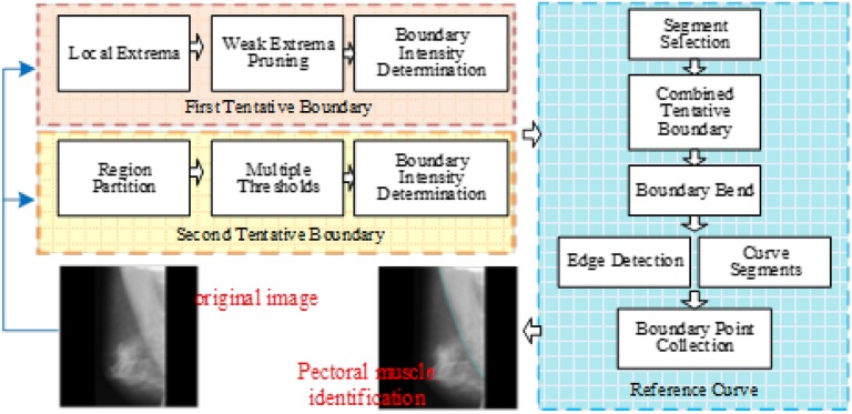
Since pectoral muscle segmentation requires the identification of the pectoral muscle in the mammogram, this research issue can be transformed into the question of breast boundary identification between the breast and pectoral muscle. The rationale of the proposed method is briefly described as follows: the tentative pectoral muscle boundary is detected as the first boundary. Then, another boundary curve is identified by another method. If the two boundary curves have a great difference, they are used to result in the final boundary. The framework of the proposed method is shown in Figure 1. The proposed method starts with the extraction of the region of interest (ROI) (i.e. the breast and the pectoral muscle) in a MLO mammogram. Two tentative boundary curves are individually created to be the potential boundaries. To find the first tentative boundary, this study finds local extrema, prunes weak extrema and then determines an appropriate threshold for identifying the brighter tissue, whose edge is considered the first tentative boundary. The second tentative boundary is found by partitioning the breast into several regions, where each local threshold is tuned based on the local intensity. Subsequently, both of the tentative boundaries are used as the reference to create a refined boundary by Hough transform. Then, the refined boundary is partitioned into quadrilateral regions, in which the edge of this boundary is detected. Finally, these reliable edge points are collected to generate the genuine boundary by curve fitting.

Figure 1.

The framework of the proposed method.

Extracting region of interest

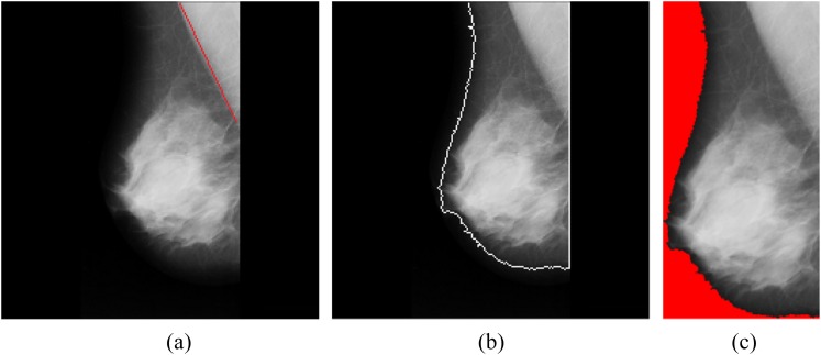
A typical MLO mammogram contains a breast and a background. The non-black pixels represent the breast tissue in the mammogram, whereas the black and near-black pixels are the background of the image. The first step of this study is to identify the breast tissue as the ROI in the image by using the region-growing method. The region-growing method starts with a set of the minimal pixel values (i.e. seed points) to group neighbouring pixels with similar pixel values. Similar pixels are iteratively grouped until the region-growing rate exceeds a pre-defined threshold at the region-growing step. In this study, the pre-defined threshold is set as 25 because the background is normally visually close to black. The bright part is regarded as the foreground of the image, whereas the dark part is the background. The minimum bounding box of the foreground is extracted to be the ROI, and the background region is not used for the subsequent processing of this study. The process of extracting the ROI is shown in Figure 2, where Figure 2a is the original mammogram. The boundary of the ROI is identified in Figure 2b. Figure 2c shows the minimum bounding box of the foreground of the image, where the red region is the ignored background.

Figure 2.

(a) Original mammogram; (b) the region of interest is identified; (c) the minimum bounding box of the region of interest.

First tentative boundary

To find the boundary for extracting out the pectoral muscle, the ROI is used to create a histogram H of the gray-level pixels, showing the number of pixels in an image at each different gray-level value i, $\forall i\in \left[\text{0,}255\right]$ found in that image. The method of detecting the first tentative boundary is described in the following subsections.

Local extrema detection

Local extrema, known as maxima or minima, are those points located at the hill and the valley along a curve. The corresponding gray-level values of the local maxima L_max can be found as follows:

$$L_{\text{max}}=i|\underset{i}{\text{argmax}}\hspace{0.17em}H\left(i\right),i\in \left[i-m,i+m\right]$$ (1)

Where i represents the ascending-sort i^th element in L_max, and m is a constant. To find the local minimum L_min between the two neighbouring maximum points $L_{\max }^j$ and $L_{\max }^{j+1}$, the method for corresponding gray-level values is expressed as follows:

$$L_{\text{min}}=i|\underset{i}{\text{argmin}}\hspace{0.17em}H\left(i\right),i\in \left[L_{\text{max}}^j,L_{\text{max}}^{j+1}\right]$$ (2)

Pruning weak extrema

The purpose of the first tentative boundary is to determine a global threshold from the histogram H. However, those weak extrema of the histogram H is likely to impede the determination of the global threshold. Those weak extrema must be removed in order to find the optimal global optimal threshold.

The way to prune these weak local maxima and minima is to calculate the differences between the minimum intensity of each region and its left and right neighbouring maximum. The product D_i of the two differences is then computed as follows:

$$D_i=\left(H\left(L_{\text{max}}^j\right)-H\left(L_{\text{min}}^{i,j}\right)\right)\times \left(H\left(L_{\text{max}}^{j+1}\right)-H\left(L_{\text{min}}^{i,j}\right)\right)$$ (3)

Where $L_{\min }^{i,j}$ represents the i^th element of ascending sort in the set L_min which belongs to $\left[L_{\max }^j,L_{\max }^{j+1}\right]$. The next step is to prune the corresponding $L_{\min }^{i,j}$ of the minimum D_i in L_min and $\min \left(L_{\max }^i,L_{\max }^{j+1}\right)$ in L_max, respectively.

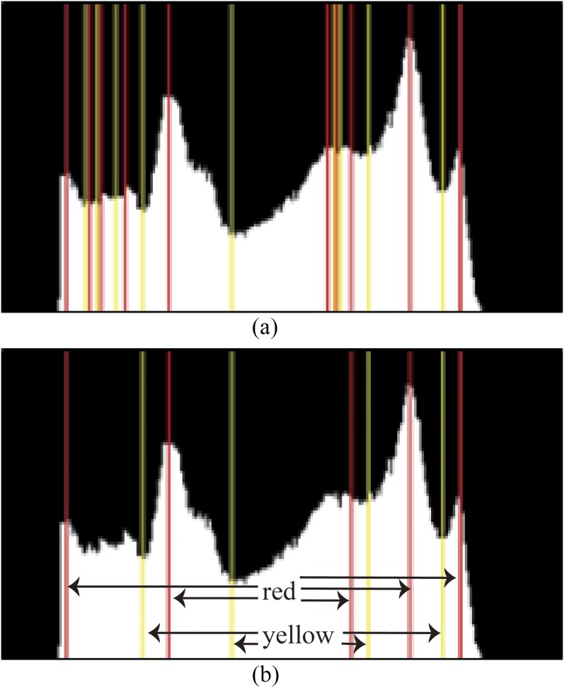
If $L_{\max }^j$ is pruned, the search process goes back to the step in Equation (2) to search for the corresponding gray-level value of the minimum within the region $\left[L_{\max }^{j-1},L_{\max }^j\right]$. If $L_{\max }^{j+1}$ is pruned, the proposed method searches for the corresponding gray-level value of the minimum within the region $\left[L_{\max }^j,L_{\max }^{j+1}\right]$. The search process is iterated until only N elements are left in L_min. The two parameters m = 3 and N = 4 were set from the empirical experiments. N must be an appropriate value in searching for the minimum or maximum. If N is too greater, relatively more elements are left, thereby losing global meaning. If N is too less, this loses the local meaning. The result of pruning weak local maxima and minima is shown in Figure 3, in which red lines and yellow lines represent local maxima and local minima, respectively. The Figure 3a shows the detected local maxima and minima in the histogram, whereas Figure 3b is the result of pruning the weak local maxima and minima using the aforementioned method. Note that the pixels in gray level ≤30 are ignored because they are the background of the mammogram without any feasible meaning.

Figure 3.

Pruning weak extrema. (a) The detected local maxima in red and minima in yellow; (b) pruning of weak local maxima and minima. For colour image see online.

Threshold determination

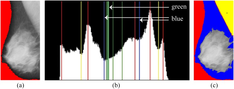
In a mammogram, the pectoral muscle and the glandular tissues are not only separated but are also brighter than other regions within the breast. If the two regions are individually extracted out from the mammogram, the pectoral muscle region can be identified through the spatial information. The pectoral muscle is located at the upper right/left of a mammogram, whereas the glandular tissues are at the lower left/right. With the prior knowledge, a threshold representing the first tentative boundary is found through the gray intensity histogram as follows. A local minimum is used to identify the greatest region of the pectoral muscle which meets the spatial features of the pectoral muscle. Another local minimum is the maximal value in the set L_min, but does not meet the spatial features of pectoral muscle. The two regions are likely to be the pectoral muscle and the glandular tissues. Finally, a binary search method⁵² is used to determine a threshold for partitioning the transition between the two local minima, which is the intensity of the boundary of the pectoral muscle. Figure 4 shows the process of conducting the first tentative boundary. Figure 4a is used to create a histogram of image intensity shown in Figure 4b, where two local minima and the intensity of the boundary are represented in blue lines and a green bold line, respectively. In Figure 4c, the black point in the yellow region represents the centroid of this region, whose spatial position is (357.6, 135.0) in this image. The boundary orientation is 63.10°, which is roughly estimated by fitting these boundary points as a straight line.

Figure 4.

Detection of the first tentative boundary. (a) A region of interest is used to create a histogram; (b) the bold line is the intensity of boundary in the mammogram; (c) results of identifying the first tentative boundary.

Second tentative boundary

Owing to the vagueness of the boundary of the pectoral muscle, the second tentative boundary serves as an alternative reference. This method can not only deal with the case of boundary vagueness but also increase the stability of the proposed method for verifying the boundary of the pectoral muscle. The method of detecting the second tentative boundary is as follows.

Region partition

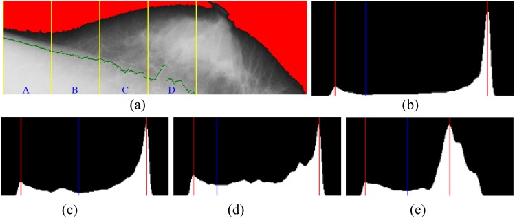
To easily observe the details of the breast structure in the subsequent process, the ROI image is rotated to the orientation in which the breast nipple is towards the top. In the left-half/right-half side of the ROI, each vertical line goes across the pectoral muscle and breast tissue, where the pixels show two different gray-level distributions. It is assumed that a ROI shows a bimodal distribution of gray-level values, which contains the two statistical modes pectoral muscle and breast tissue. Since most of the side region shows strong contrast between the pectoral muscle and breast tissue, it is relatively easy to find a point at which to partition the bimodal. For this reason, the ROI can be divided into several regions. In this study, the ROI is divided into four regions with an equal width. The intensity of each region is used to create individual histograms, where the horizontal axis represents intensity variations while the vertical axis is the number of pixels in that particular intensity.

Multiple thresholds

In a bimodal histogram, a threshold can be found to partition the bimodal distribution into two separate models. The threshold represents the tentative boundary for the given region. Figure 5 shows that gray-level histograms of the selected regions were created to determine the thresholds. Figure 5a shows that a ROI is divided into four regions A, B, C and D. The gray-level histograms of the separate regions were created to determine the thresholds.⁵³

Figure 5.

Gray-level histograms of the selected regions were created to determine the thresholds. (a) The region of interest is divided into four regions: A, B, C and D; (b) Threshold_A = 68 for Region A; (c) Threshold_B = 118 for Region B; (d) Threshold_C = 66 for Region C; (e) Threshold_D = 94 for Region D.

A pectoral muscle boundary in a ROI is expressed as a curve, where points are connected with their neighbouring points. Even if the curve is divided into several regions, the continuity property still exists between any two neighbouring regions. This property motivates the researchers of this study to use the stable line segment at the side-most region as a reference to calibrate the line segment at the neighbouring region.

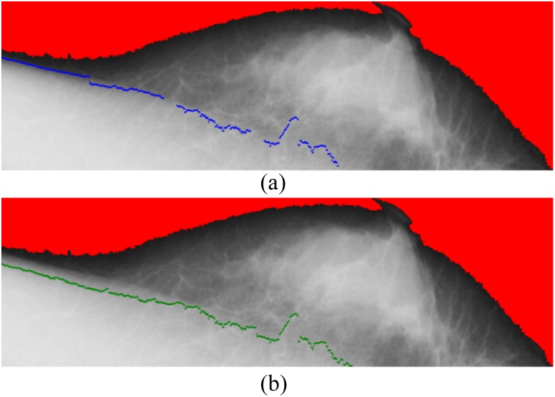
In Figure 6, the cyan points represent the corresponding pixels of the threshold for each region. The cyan points compose the second boundary, whereas the green points show the initial boundary detected at the previous stage. Figure 7 shows the results on detection of the pectoral muscle boundary by the proposed multiple thresholds and the single threshold. In Figure 7a, the boundary was detected by multiple thresholds and drawn in blue; in Figure 7b, the boundary was detected by the single threshold and drawn in green. In comparison, the boundary detected by multiple thresholds is closer to the ground truth than that detected by the single threshold. Figure 8 shows how the line segments are connected. The line segment close to the breast boundary is retained as the line segment at Region A. The line segment at Region A is extended to Region B. At Region B, the line segment close to the line segment of Region A is retained. Figure 8 shows that the line segment at Region A determines the line segment at Region B. The selected line segments at Regions A and B conduct curve fitting to generate a curve. The resulting curve at Regions A and B is used as the reference for the line segment at Region C. Once again, the resulting curve at Regions A, B and C is used to determine the line segment at Region D.

Figure 6.

The cyan points represent the corresponding pixels of the threshold for each region. The cyan points compose the second boundary, whereas the green points show the first boundary detected at the previous stage. For colour image see online.

Figure 7.

Results on detection of pectoral muscle boundary by single and multiple thresholds. (a) The boundary was detected by multiple thresholds and drawn in blue; (b) the boundary was detected by the single threshold and drawn in green. For colour image see online.

Figure 8.

The blue line segments are retained. For colour image see online.

Segment selection

At this stage, each divided region of the ROI contains two line segments, the first tentative boundary and the second tentative boundary. A detected line segment near the boundary is selected for fitting the curve of the whole boundary. As described in the previous section, the orientation of the line segment must meet the condition that the pectoral muscle boundary is located within the defined orientation. In the right breast MLO mammogram, the orientation of the pectoral muscle falls between −35° and −85°, whereas the orientation is between 35° and 85° in the left breast MLO mammogram. If the two line segments both meet the orientation requirement, the line segments with the lower gray level will be selected as the final line segment.

Reference curve by curve fitting

The reference curve at each region is created by the curve-fitting method. In each region, the points along the selected line segment are fitted into a second degree polynomial equation, expressed in Equation (4):

$$y=c_0{x}^2+c_{1}x+c_2$$ (4)

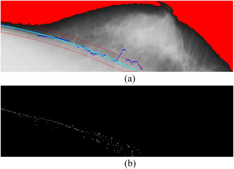
where c_i (i = 0, 1, 2) are parameters computed by the least squares method. If the farthest point from the line segment falls beyond three standard deviations of the mean, this point is seen as an outlier and removed from the set. The curve-fitting process is iterated until all points reach the requirement that the residual of each point is less than three. Once the reference curve is simulated, its band is also created, which is set as 30 pixels. The edge detection of the band of the reference curve was performed using the Sobel operator. Among the edge points, the three greatest values in magnitude were retained in each vertical line (Figure 9).

Figure 9.

(a) Fitting the curve and determining the regional band; (b) sampling the points within the regional band.

Since a set of pixels may partially describe the boundary of the pectoral muscle, the Hough transform can be used to simulate the curve. The Hough transform, introduced in 1962⁵⁴ and first used to find lines in images,⁵⁵ can be used to detect parametric curves. The Hough transform defines a mapping transformation between the image space and the ρ − θ parameter space using a polar co-ordinate system. This parameterization shows a straight line of the image space (i.e. the x − y space) by the orientation θ between its normal vector and the x-axis, and its algebraic distance ρ from the origin (0,0). The straight line corresponding to this geometry can be described as:

$$\rho =x\text{cos}\left(\theta \right)+y\text{sin}\left(\theta \right)$$ (5)

Considering θ ∈ [−90°; 90°], given a straight line γ in the image space with its respective ρ and θ parameters, say ρ₀ and θ₀, it is represented in the ρ − θ space by a single point, with co-ordinates $\left({\rho }_{\text{0}},{\theta }_0\right)$. Each point, with co-ordinates (x,y) in the image space, is represented by a sinusoidal curve in the ρ − θ space following Equation (5). It is easy to show that in the parameter space, the sinusoidal curves that correspond to points belonging to γ have a common intersection point $\left({\rho }_0,{\theta }_0\right)$. Based on this relationship, the problem of detecting straight lines in the image space can be converted into the problem of identifying intersection peaks in the parameter space. When working in a discrete space, one can represent the parameter space by an accumulator matrix. Furthermore, to find straight lines in the image, it is necessary to find peaks (i.e. positions with high values) in the accumulator matrix. The results are illustrated in Figure 10.

Figure 10.

Hough transform of edge points within the edge band.

With the features, the piecewise linear representation (PLR) algorithm is utilized to collect the potential edge points as follows:

Initial set: collect the curve points in sequence P.

The leftmost point is assigned as 1, and the rightmost point is N.

The set ξ = {1, N} with the threshold. The PLR algorithm⁵⁶ is designed as follows:

$$\text{PLR}\left(P,i\text{Bgn},i\text{End},\xi ,\text{Threshold}\right)$$

Begin

$$\text{Let}\hspace{0.17em}{p}_b=P\left(i\text{Bgn}\right),p_e=P\left(i\text{End}\right)$$

Create a line between P_b and P_e

$$\text{Sort all points along the line}\hspace{0.17em}\overline{P_b{P}_e}\hspace{0.17em}\text{and within the}\hspace{0.17em}\left[i\text{Bgn},i\text{End}\right]$$

$$\text{Find the farthest point}\hspace{0.17em}P\left(i\right)\hspace{0.17em}\text{with the distance}\hspace{0.17em}d,\text{in the region}\hspace{0.17em}\left[i\text{Bgn},i\text{End}\right]$$

If d < Threshold Then stop

Else

Put P(i) into ξ

$$\text{If}\hspace{0.17em}i\text{\hspace{0.17em}−\hspace{0.17em}}i\text{Bgn\hspace{0.17em}≥\hspace{0.17em}2 Then PLR}\left(P,i\text{Bgn},i,\xi ,\text{Threshold}\right)$$

$$\text{If}\hspace{0.17em}i\text{End\hspace{0.17em}−\hspace{0.17em}}i\text{\hspace{0.17em}≥\hspace{0.17em}2 Then PLR}\left(P,i,i\text{End},\xi ,\text{Threshold}\right)$$

End If

End

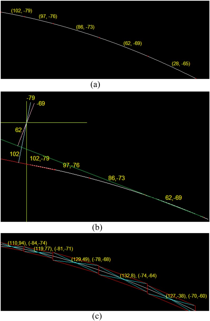
This study computes the (γ,θ) of the Hough transform of each segmental line with threshold = 2 and $\xi =\left\{p_1,p_2\dots ,p_n\right\}$. The results are shown in Figure 11. The figures in parentheses in Figure 11 represent the corresponding (γ,θ) of the Hough transform of the given segment between the two red points. The co-ordinate (γ,θ) corresponds to the position in the image. Taking Figure 11 as an example, the co-ordinate (0,0) is the upper left of the image. In the co-ordinate $\left(102,-79°\right)$, the first figure 102 indicates the distance on this segmental curve between the position (0,0) and the red point. The second figure −79° is the orientation between the segmental curve and the horizontal axis.

Figure 11.

(a) ρ − θ space; (b) the image space; (c) quadrilateral regions are defined for each line segment.

The technical meanings of Figure 11a–c are indicated as follows. In Figure 11a, the six red points represent end points of line segments, determined by the PLR method. Through the Hough transform, each line segment is associated with a set of parameters (ρ,θ). For example, (102, −79) is a parametric set from the Hough transform. Figure 11b illustrates the relationship between the set of (ρ,θ) and the co-ordinate system used for the image, where the origin of the co-ordinate system is shown at the upper left of the image, and the first quadrant is located at the lower right of the origin. The rightmost point (102,−79) of the red tentative curve is extended as a straight red line, whose shortest distance to the origin is 102. The distance is computed by drawing the blue perpendicular line from the red line to the origin. The orientation between the light blue line and the horizontal axis is −79°, shown as the shorter red arrows. This method is also used for the other points of the tentative curve in green. The green straight line is extended from the point (62,−69) and the magenta line is drawn to compute the shortest distance and the orientation. Figure 11c shows the method for sampling reliable data points. The method firstly partitions the tentative curve into several line segments and then sets the middle of each line segment as the centre point. As each line segment based on the centre point rotates ±α (α = 5° in this study), each point can result in a quadrilateral region. Those located within the quadrilateral region can be seen as the reliable points for curve fitting.

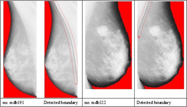
Once the quadrilateral regions are determined, the points located within the quadrilateral regions can be collected for curve fitting in a fifth order polynomial, making it possible to create more bending for the boundary of the pectoral muscle. In Figure 12, the red points are used for curve fitting, whereas the green points are discarded. The advantage of the proposed method is to identify the boundary between the obscure pectoral muscles. Figure 13 shows that the pectoral muscles boundary can be found on each mammogram although the boundary is obscure.

Figure 12.

The red points are used for curve fitting, whereas the green points are discarded. For colour image see online.

Figure 13.

The pectoral muscles boundary is identified on each mammogram though the boundary is obscure.

Performance evaluation

For the boundary identification of the pectoral muscle, this study compares the performance of the proposed method with two other methods, the methods by Ferrari et al²⁹ and Liu et al⁴⁷. The boundary of the pectoral muscle can also be seen as a curve for this research issue. For this reason, the simulation results of a polynomial curve using sampling points are evaluated. The boundary of the pectoral muscle in each mammogram was manually delineated by a senior researcher who has at least 5 years' of experience in digital mammogram processing and analysis. The delineative curves of the pectoral muscle boundary are used as the standard of reference to evaluate the proposed method and earlier methods for the detection of the pectoral muscle. Mean square error (MSE) is a measure of the differences between the values predicted by an estimator and the values actually observed from the curve modeled.⁵⁷ An MSE value indicates the stability of the segmentation quality in breast images. As the MSE of the curve-fitting method is less, its performance quality is better.

$$\text{MSE}=\frac{{\displaystyle \sum _{i=1}^n{\left({\left(x_{Gi}-x_{Mi}\right)}^2+{\left(y_{Gi}-y_{Mi}\right)}^2\right)}^{\frac{1}{2}}}}{n}$$ (6)

where $\left(x_{Gi},y_{Gi}\right)$ represents the i^th data point of the ground truth, and $\left(x_{Mi},y_{Mi}\right)$ is the nearest data point from $\left(x_{Gi},y_{Gi}\right)$.

In addition, the boundary segmentation of the pectoral muscle can be regarded as a binary classification problem. The misclassification error rate (MER), the percent of misclassified records out of the total records in the validation data, is estimated using Equation (7):

$$\text{MER}=\frac{\text{FN}+\text{FP}}{\text{TP}+\text{FN}+\text{TN}+\text{TP}}$$ (7)

where TP, TN, FP and FN represent true positive, true negative, false positive and false positive, respectively. The relative foreground area error (RFAE) indicates the region mismatch between the extracted object and the ground truth object and is defined in Equation (8)

$$\text{RFAE}=\{\begin{array}{cc}\frac{\left(\text{TP}+\text{FN}\right)-\left(\text{FP}+\text{TP}\right)}{\text{TP}-\text{FN}}=\frac{\text{FN}-\text{FP}}{\text{TP}+\text{FN}}& \text{if}\left(\text{FP}+\text{TP}\right)<\left(\text{TP}+\text{FN}\right)\\ \frac{\left(\text{FP}+\text{FN}\right)-\left(\text{TP}+\text{FN}\right)}{\text{FP}+\text{TP}}=\frac{\text{FP}-\text{FN}}{\text{FP}+\text{TP}}& \text{if}\left(\text{FP}+\text{TP}\right)\ge \left(\text{TP}+\text{FN}\right)\end{array}$$ (8)

The extraction error rate (EER) expresses the failure rate of the algorithm in Equation (9).

$$\text{EER}=\text{FN}/\left(\text{TP}+\text{FN}\right)+\text{FP}/\left(\text{TP}+\text{FN}\right)$$ (9)

RESULTS

In the experiments of this study, the breast images were selected from the database of the Mammographic Images Analysis Society.⁵⁸ The size of each image is 1024 × 1024 pixels. All of the images have been annotated for class, severity and location of abnormality, character of background tissue, and radius of circle enclosing the abnormality.

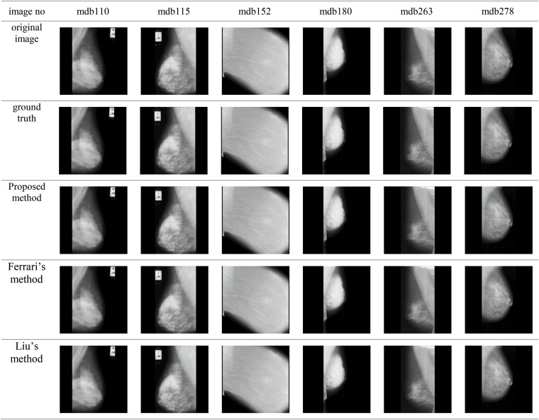
This study compares the performance of the proposed method with the methods be Liu et al and Ferrari et al. In the method by Liu et al, the region of the pectoral muscle is roughly identified by recursively finding the threshold of the image intensity. Intensities greater than the threshold are considered the potential pectoral region, whereas intensities less than the threshold are the background. The recursion process is ended when the region at two consecutive iterations varies by <5%. Then, the morphological erosion method is used to separate the pectoral muscle from the breast as well as to remove noise. Finally, the pectoral muscle boundary is simulated by the fifth order polynomial curve fitting. Figure 14 shows the results of the proposed method and the compared methods for identifying pectoral muscle in the mammogram.

Figure 14.

Results of the proposed method and the compared methods for identifying pectoral muscle in the mammogram.

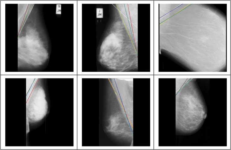
The method by Ferrari et al is based on two assumptions. The first assumption is that the pectoral muscle boundary is a straight line within the orientation range [120–170°]. The second assumption is that the pectoral muscle displays as brighter than the breast region. Furthermore, the gray level of this region is relatively high compared with the other regions of the breast. With these two assumptions, Ferrari et al used the Sobel operator to detect the pectoral muscle boundary, and then applied the Hough transform to find the potential straight line. The major drawback of this method is that the pectoral muscle may not be a straight line. In addition, this method can generate >4000 straight lines using the Hough transform. Based on the selection criteria, the six best potential lines were selected to be shown in Figure 15, where the green line is the optimal one. Both the upper leftmost and lower leftmost images show fair results, where the resulting lines are close to the actual boundary. For the other four images, the resulting lines are limited to the second assumptions. This method can obtain fair boundary results only if the pectoral muscle is present in a straight line. When this method applied the Hough transform on an image, >4000 straight lines were created for each image. Based on the criteria proposed by Ferrari et al, the best six pectoral muscle lines were selected from these resulting lines, as shown in Figure 15.

Figure 15.

The best six pectoral muscle lines proposed based on the method by Ferrari et al.²⁹

Table 1 shows the MSE in mean, maximum and minimum for the three different methods, the proposed method and those by Ferrari et al and Liu et al. Among the three methods, the proposed method achieves the least MSE of 4.88 ± 2.47 (mean ± standard deviation), indicating that this method performs best and stably in boundary identification of the pectoral muscle. Tables 2–4 show the comparison of the different methods in terms of the relative foreground area error (RFAE), misclassification error rate (MER) and extraction error rate (EER). The proposed method still achieves the least RFAE, MER and EER among the three methods.

Table 1.

Comparison of different methods on mean square error in mean, maximum, minimum

Image number	Ferrari et al29	Liu et al47	Proposed method
mdb110	(33.16, 70.38, 0.00)	(6.85, 21.93, 0.00)	(5.53, 14.87, 0.00)
mdb115	(60.55, 116.50, 0.00)	(30.15, 35.23, 25.00)	(0.75, 3.16, 0.00)
mdb152	(135.40, 326.00, 0.00)	(39.10, 86.37, 2.00)	(8.00, 22.02, 0.00)
mdb180	(59.36, 61.85, 55.71)	(13.68, 28.30, 3.00)	(4.56, 12.00, 0.00)
mdb263	(15.74, 69.06, 0.00)	(28.78, 40.31, 1.41)	(3.08, 12.04, 0.00)
mdb278	(19.88, 66.85, 0.00)	(7.98, 16.00, 0.00)	(7.33, 19.00, 0.00)
Mean ± standard deviation	54.02 ± 40.33	21.09 ± 12.21	4.88 ± 2.47

Table 2.

Comparison of different methods on the relative foreground area error (RFAE)

Image number	Ferrari et al29	Liu et al47	Proposed
mdb110	0.29163	0.05487	0.05158
mdb115	0.36020	0.18037	0.00118
mdb152	0.17508	0.35756	0.06938
mdb180	0.56591	0.91347	0.05439
mdb263	0.04856	0.18036	0.01259
mdb278	0.32116	0.05487	0.10240
Mean ± standard deviation	0.293757 ± 0.159918	0.29025 ± 0.296617	0.0048587 ± 0.033946

Table 4.

Comparison of different methods on extraction error rate (EER)

Image number	Ferrari et al29	Liu et al47	Proposed
mdb110	0.30451	0.06384	0.05203
mdb115	0.39261	0.18037	0.00461
mdb152	0.89216	0.35756	0.07272
mdb180	0.56591	10.55731	0.05581
mdb263	0.08235	0.18036	0.01677
mdb278	0.41742	0.06384	0.10263
Mean ± standard deviation	0.442493 ± 0.24809	1.900547 ± 3.872669	0.050762 ± 0.032876

Table 3.

Comparison of different methods on misclassification error rate (MER)

Image number	Ferrari et al29	Liu et al47	Proposed
mdb110	0.02819	0.00591	0.00482
mdb115	0.07995	0.03673	0.00094
mdb152	0.05422	0.02173	0.00442
mdb180	0.04897	0.91347	0.00483
mdb263	0.02770	0.03673	0.00564
mdb278	0.02964	0.00591	0.00729
Mean ± standard deviation	0.04478 ± 0.01889	0.17008 ± 0.33269	0.00466 ± 0.00191

DISCUSSION

Effectiveness of multiple thresholds for region partition: the proposed method attempts to find the thresholds of individually smaller regions as the second tentative boundary. The boundary detected by the multiple thresholds is closer to the ground-truth than that detected by the singular threshold of the whole region because fewer errors or outliers in the smaller regions were introduced in the process of determining the threshold. The results in this study demonstrate the advantages of the multiple thresholds and the region partition.

Simulation of the curve or straight line

In most cases, the pectoral muscle boundary is present as a curve. To precisely simulate such a curve, this study partitions the whole boundary into several smaller segments, simulates the curves individually and then connects the individual curves to form a singular curve. For the case where the pectoral muscle is almost a straight line in the mammogram, this method can also generate that straight line because a straight line is a special case of a curve with curvature = 0. This proposed method can still perform well in the cases of both a straight line and a curve.

Disturbance of noise

The points for curve fitting are the key to simulating the shape of the fit curve. To prevent disturbance of noise, the sample boundary points were only collected from the quadrilateral regions. In addition to the limitation of the sampling region, another way is to increment not only the Hough accumulator cell $\text{Acc}\left({\theta }_i,{\gamma }_i\right)$ for a given orientation θ but also the neighbouring cells $\left({\theta }_{i+1},{\gamma }_i\right)$ and $\left({\theta }_i,{\gamma }_{i+1}\right)$. This makes the Hough transform more tolerant against inaccurate point co-ordinates.

Setting of parameter α for size of quadrilateral regions

The setting of parameter α is associated with the area size of the quadrilateral region. As parameter α is small, the resulting area becomes small, thereby narrowing the region of sampling points. The resulting curve is likely to be closer to the tentative curve. Another idea is that each quadrilateral region can also set its own parameter α, which is appropriate to its sampling requirement. As the mechanism is applied to the mammograms, where the upper breast and the upper pectoral muscle are clearer than the lower parts, more points were collected from these clear parts than from the obscure parts.

Image contrast in breasts

Since the intensity-based methods attempt to identify the regions with different intensities, the performance of the compared method is greatly affected by image contrast. This can explain why the methods by Liu et al and Ferrari et al cannot work well on number mdb152, because it is present in low contrast. The proposed method can work well because two tentative boundaries are utilized for two-step verification.

CONCLUSIONS

The contributions of this study are two-fold. First, a novel method was proposed to identify and segment the pectoral muscle in X-ray MLO mammograms. The proposed method does not straightforwardly detect the boundary curve of the pectoral muscle due to the obscure image content. Instead, it narrows down the curve region and finds the curve orientation step by step. Second, a method is proposed to sample reliable points from the noisy space for curve fitting. The experimental results indicate that the proposed simulation method can perform better than the other edge detection methods in terms of the RME, meaning that the fitting curve can be close to the boundary delineated by the medical doctor.

FUNDING

This work was supported by Ministry of Science and Technology, Taiwan, under research project number MOST 104-2221-E-231-010.

REFERENCES

- 1.Breastcancer.org. Breast cancer statistics; 2011.[Cited 22 March 2016.] Available from: http://www.breastcancer.org/symptoms/understand_bc/statistics [Google Scholar]
- 2.DeSantis C, Ma J, Bryan L, Jemal A. Breast cancer statistics, 2013. CA Cancer J Clin 2014; 64: 52–62. doi: 10.3322/caac.21203 [DOI] [PubMed] [Google Scholar]
- 3.National Cancer Institute. Mammograms; 2010. [Cited 22 March 2016.] Available from: http://www.cancer.gov/types/breast/mammograms-fact-sheet [Google Scholar]
- 4.US Preventive Services Task Force. Screening for breast cancer: U.S. Preventive Services Task Force recommendation statement. Ann Intern Med 2009; 151: 716–26. doi: 10.7326/0003-4819-151-10-200911170-00008 [DOI] [PubMed] [Google Scholar]
- 5.Dromain C, Boyer B, Ferré R, Canale S, Delaloge S, Balleyguier C. Computed-aided diagnosis (CAD) in the detection of breast cancer. Eur J Radiol 2013; 82: 417–23. doi: 10.1016/j.ejrad.2012.03.005 [DOI] [PubMed] [Google Scholar]
- 6.Ganesan K, Acharya UR, Chua KC, Min LC, Abraham KT. Pectoral muscle segmentation: a review. Comput Methods Programs Biomed 2013; 110: 48–57. doi: 10.1016/j.cmpb.2012.10.020 [DOI] [PubMed] [Google Scholar]
- 7.Bick U, Giger ML, Schmidt RA, Nishikawa RM, Wolverton DE, Doi K. Automated segmentation of digitized mammograms. Acad Radiol 1995; 2: 1–9. [DOI] [PubMed] [Google Scholar]
- 8.Byng JW, Boyd NF, Fishell E, Jong RA, Yaffe MJ. Automated analysis of mammographic densities. Phys Med Biol 1996; 41: 909–23. doi: 10.1088/0031-9155/41/5/007 [DOI] [PubMed] [Google Scholar]
- 9.Méndez AJ, Tahoces PG, Lado MJ, Souto M, Correa JL, Vidal JJ. Automatic detection of breast border and nipple in digital mammograms. Comput Methods Programs Biomed 1996; 49: 253–62. [DOI] [PubMed] [Google Scholar]
- 10.Goodsitt MM, Chan HP, Liu B, Guru SV, Morton AR, Keshavmurthy S, et al. Classification of compressed breast shapes for the design of equalization filters in X-ray mammography. Med Phys 1998; 25: 937–48. doi: 10.1118/1.598272 [DOI] [PubMed] [Google Scholar]
- 11.Heine J, Kallergi M, Chetelat S, Clarke L. Multiresolution wavelet approach for separating the breast region from the background in high resolution digital mammography. In: Karssemeijer N, Thijssen M, Hendriks J, van Erning L, eds. Digital mammography. Houten, Netherlands: Springer; 1998. pp. 295–8. [Google Scholar]
- 12.Karssemeijer N, Te Brake G. Combining single view features and asymmetry for detection of mass lesions. In: Karssemeijer N, Thijssen M, Hendriks J, van Erning L. eds. Digital mammography. Houten, Netherlands: Springer; 1998. pp. 95–102. [Google Scholar]
- 13.Kwok SM, Chandrasekhar R, Attikiouzel Y. Automatic pectoral muscle segmentation on mammograms by straight line estimation and cliff detection. The Seventh Australian and New Zealand 2001 Intelligent Information Systems Conference; 18–21 November 2001; Perth, WA, Australia. New York, NY: IEEE Engineering in Medicine and Biology Society, 2001. pp. 67–72.
- 14.Grau V, Mewes AU, Alcañiz M, Kikinis R, Warfield SK. Improved watershed transform for medical image segmentation using prior information. IEEE Trans Med Imaging 2004; 23: 447–58. doi: 10.1109/TMI.2004.824224 [DOI] [PubMed] [Google Scholar]
- 15.Thangavel K, Karnan M. Computer aided diagnosis in digital mammograms: detection of microcalcifications by meta heuristic algorithms. ICGST Int J Graphics Vis Image Process 2005; 5: 41–55. [Google Scholar]
- 16.Raba D, Oliver A, Martí J, Peracaula M, Espunya J. Breast segmentation with pectoral muscle suppression on digital mammograms. In: Marques J, Pérez de la Blanca N, Pina P, eds. Pattern recognition and image analysis. Heidelberg, Germany: Springer; 2005. pp. 471–8. [Google Scholar]
- 17.Mirzaalian H, Ahmadzadeh MR, Sadri S. Pectoral muscle segmentation on digital mammograms by nonlinear diffusion filtering. IEEE Pacific Rim Conference on Communications, Computers and Signal Processing; 22–24 August 2007; Victoria, BC. New York, NY: IEEE Press; 2007. pp. 581–4.
- 18.Yapa RD, Koichi H. A connected component labeling algorithm for grayscale images and application of the algorithm on mammograms. Proceedings of the 2007 ACM Symposium on Applied Computing; 11–15 March 2007. Seoul, Republic of Korea: New York, NY: ACM Press; 2007. pp. 146–52.
- 19.Hong BW, Sohn BS. Segmentation of regions of interest in mammograms in a topographic approach, IEEE Trans Inf Technol Biomed 2010; 14: 129–39. doi: 10.1109/TITB.2009.2033269 [DOI] [PubMed] [Google Scholar]
- 20.Nagi J, Abdul Kareem S, Nagi F, Ahmed SK. Automated breast profile segmentation for ROI detection using digital mammograms. IEEE EMBS Conference on Biomedical Engineering and Sciences (IECBES); 30 November–2 December 2010; Kuala Lumpur, Malaysia. New York, NY: IEEE Press; 2010. pp. 87–92.
- 21.Saltanat N, Hossain MA, Alam MS. An efficient pixel value based mapping scheme to delineate pectoral muscle from mammograms. 2010 IEEE Fifth International Conference on Bio-Inspired Computing: Theories and Applications (BIC-TA); 23–26 September 2010; Changsha, China. New York, NY: IEEE Press; 2010. pp. 1510–17.
- 22.Sultana A, Ciuc M, Strungaru R. Detection of pectoral muscle in mammograms using a mean-shift segmentation approach. The 8th International Conference on Communications (COMM); 10–12 June 2010; Bucharest, Romania. New York, NY: IEEE Press; 2010. pp. 165–8.
- 23.Camilus KS, Govindan VK, Sathidevi PS. Pectoral muscle identification in mammograms. J Appl Clinl Med Phys 2011; 12: 3285. [DOI] [PMC free article] [PubMed] [Google Scholar]
- 24.Molinara M, Marrocco C, Tortorella F. Automatic segmentation of the pectoral muscle in mediolateral oblique mammograms. IEEE 26th International Symposium on Computer-Based Medical Systems (CBMS); 20–22 June 2013; Porto, Portugal. New York, NY: IEEE Press; 2013. pp. 506–9.
- 25.Mustra M, Grgic M. Robust automatic breast and pectoral muscle segmentation from scanned mammograms. Signal Process 2013; 93: 2817–27. doi: 10.1016/j.sigpro.2012.07.026 [DOI] [Google Scholar]
- 26.Li Y, Chen H, Yang Y, Yang N. Pectoral muscle segmentation in mammograms based on homogenous texture and intensity deviation. Pattern Recogn 2013; 46: 681–91. doi: 10.1016/j.patcog.2012.09.021 [DOI] [Google Scholar]
- 27.Karssemeijer N. Automated classification of parenchymal patterns in mammograms. Phys Med Biol 1998; 43: 365. doi: 10.1088/0031-9155/43/2/011 [DOI] [PubMed] [Google Scholar]
- 28.Yam M, Brady M, Highnam R, Behrenbruch C, English R, Kita Y. Three-dimensional reconstruction of microcalcification clusters from two mammographic views. IEEE Trans Med Imaging 2001; 20: 479–89. doi: 10.1109/42.929614 [DOI] [PubMed] [Google Scholar]
- 29.Ferrari RJ, Rangayyan RM, Desautels JE, Borges RA, Frère AF. Automatic identification of the pectoral muscle in mammograms. IEEE Trans Med Imaging 2004; 23: 232–45. doi: 10.1109/TMI.2003.823062 [DOI] [PubMed] [Google Scholar]
- 30.Kwok SM, Chandrasekhar R, Attikiouzel Y. Automatic assessment of mammographic positioning on the mediolateral oblique view. Int Conf Image Process 2004; 151: 151–4. [Google Scholar]
- 31.Weidong X, Lihua L, Wei L. A novel pectoral muscle segmentation algorithm based on polyline fitting and elastic thread approaching. The 1st International Conference on Bioinformatics and Biomedical Engineering; 6–8 July 2007; Wuhan, China. New York, NY: IEEE Press; 2007. pp. 837–40.
- 32.Galdran A, Picón A, Garrote E, Pardo D. Pectoral muscle segmentation in mammograms based on cartoon-texture decomposition. Pattern recognition and image analysis: 7th Iberian Conference, IbPRIA 2015; 17–19 June 2015; Santiago de Compostela, Galicia, Spain. Cham Switzerland: Springer International Publishing, 2015. pp. 587–94.
- 33.Liu C-C, Tsai C-Y, Liu J, Yu C-Y, Yu S-S. A pectoral muscle segmentation algorithm for digital mammograms using Otsu thresholding and multiple regression analysis. Comput Mathe Appl 2012; 64: 1100–7. doi: 10.1016/j.camwa.2012.03.028 [DOI] [Google Scholar]
- 34.Chakraborty J, Mukhopadhyay S, Singla V, Khandelwal N, Bhattacharyya P. Automatic detection of pectoral muscle using average gradient and shape based feature. J Digit Imaging 2012; 25: 387–99. doi: 10.1007/s10278-011-9421-y [DOI] [PMC free article] [PubMed] [Google Scholar]
- 35.Dijkstra EW. A note on two problems in connexion with graphs. Numer Math 1959; 1: 269–71. doi: 10.1007/BF01386390 [DOI] [Google Scholar]
- 36.Miller P, Astley S. Classification of breast tissue by texture analysis. Image Vis Comput 1992; 10: 277–82. doi: 10.1016/0262-8856(92)90042-2 [DOI] [Google Scholar]
- 37.Boyd NF, Byng JW, Jong RA, Fishell EK, Little LE, Miller AB, et al. Quantitative classification of mammographic densities and breast cancer risk: results from the Canadian National Breast Screening Study. J Natl Cancer Inst 1995; 87: 670–5. doi: 10.1093/jnci/87.9.670 [DOI] [PubMed] [Google Scholar]
- 38.Varma M, Zisserman A. Classifying images of materials: achieving viewpoint and illumination independence. Proceedings of the 7th European Conference on Computer Vision—Part III; 29 April 2002; Copenhagen, Denmark. Heidelburg, Germany: Springer-Verlag, 2002. pp. 255–71.
- 39.Carvalho I, Luz LMS, Alvarenga AV, Infantosi AFC, Pereira WCA, Azevedo CM. An automatic method for delineating the pectoral muscle in mammograms. IV Latin American Congress on Biomedical Engineering 2007; 24–28 September 2007; Margarita Island, Venezuela. Heidelberg, Germany: Springer, 2008. pp. 271–5.
- 40.Kinoshita SK, Azevedo-Marques PM, Pereira RR, Jr, Rodrigues JA, Rangayyan RM. Radon-domain detection of the nipple and the pectoral muscle in mammograms. J Digit Imaging 2008; 21: 37–49. doi: 10.1007/s10278-007-9035-6 [DOI] [PMC free article] [PubMed] [Google Scholar]
- 41.Grim J, Somol P, Haindl M, Danes J. Computer-aided evaluation of screening mammograms based on local texture models. IEEE Trans Image Process 2009; 18: 765–73. doi: 10.1109/TIP.2008.2011168 [DOI] [PubMed] [Google Scholar]
- 42.Iglesias JE, Karssemeijer N. Robust initial detection of landmarks in film-screen mammograms using multiple FFDM atlases. IEEE Trans Med Imaging 2009; 28: 1815–24. doi: 10.1109/TMI.2009.2025036 [DOI] [PubMed] [Google Scholar]
- 43.Camilus KS, Govindan VK, Sathidevi PS. Computer-aided identification of the pectoral muscle in digitized mammograms. J Digit Imaging 2010; 23: 562–80. doi: 10.1007/s10278-009-9240-6 [DOI] [PMC free article] [PubMed] [Google Scholar]
- 44.Cardoso JS, Domingues I, Amaral I, Moreira I, Passarinho P, Santa Comba J, et al. Pectoral muscle detection in mammograms based on polar coordinates and the shortest path. Conf Proc IEEE Eng Med Biol Soc 2010; 2010: 4781–4. doi: 10.1109/IEMBS.2010.5626634 [DOI] [PubMed] [Google Scholar]
- 45.Domingues I, Cardoso JS, Amaral I, Moreira I, Passarinho P, Santa Comba J, et al. Pectoral muscle detection in mammograms based on the shortest path with endpoints learnt by SVMs. Conf Proc IEEE Eng Med Biol Soc 2010; 2010: 3158–61. doi: 10.1109/IEMBS.2010.5627168 [DOI] [PubMed] [Google Scholar]
- 46.Wang L, Zhu M-l, Deng L-p, Yuan X. Automatic pectoral muscle boundary detection in mammograms based on Markov chain and active contour model. J Zhejiang Univ Sci C 2010; 11: 111–18. [Google Scholar]
- 47.Liu L, Wang J, Wang T. Breast and pectoral muscle contours detection based on goodness of fit measure. 2011 5th International Conference on Bioinformatics and Biomedical Engineering (iCBBE); 10–12 May 2011; Wuhan, China. New York, NY: IEEE Press; 2011. pp. 1–4.
- 48.Feudjio CK, Klein J, Tiedeu A, Colot O. Automatic extraction of pectoral muscle in the MLO view of mammograms. Phys Med Biol 2013; 58: 8493–515. doi: 10.1088/0031-9155/58/23/8493 [DOI] [PubMed] [Google Scholar]
- 49.Chen X, Moschidis E, Taylor C, Astley S. A novel framework for fat, glandular tissue, pectoral muscle and nipple segmentation in full field digital mammograms. 12th International Workshop, IWDM 2014; 29 June–2 July 2014; Gifu City, Japan. Cham Switzerland: Springer International Publishing, 2014. pp. 201–8.
- 50.Al-Ghaib H, Wang Y, Adhami R. A new machine learning algorithm for breast and pectoral muscle segmentation. Eur J Adv Eng Technol 2015; 2: 21–9. [Google Scholar]
- 51.Sreedevi S, Sherly E. A novel approach for removal of pectoral muscles in digital mammogram. Procedia Comput Sci 2015; 46: 1724–31. doi: 10.1016/j.procs.2015.02.117 [DOI] [Google Scholar]
- 52.Weiss MA. Data structures and algorithm analysis in C++. Upper Saddle River, NJ:Prentice Hall; 2013. [Google Scholar]
- 53.Prewitt JM, Mendelsohn ML. The analysis of cell images. Ann N Y Acad Sci 1966; 128: 1035–53. doi: 10.1111/j.1749-6632.1965.tb11715.x [DOI] [PubMed] [Google Scholar]
- 54.Hough PVC. Method and Means for Recognizing Complex Patterns, US Patent 3 069 654. 1962. [Cited 22 March 2016.] Available from: http://www.google.com.tw/patents/US3069654 [Google Scholar]
- 55.Duda RO, Hart PE. Use of the Hough transformation to detect lines and curves in pictures. Commun ACM 1972; 15: 11–15. doi: 10.1145/361237.361242 [DOI] [Google Scholar]
- 56.Wu H, Salzberg B, Zhang D. Online event-driven subsequence matching over financial data streams. Proceedings of the 2004 ACM SIGMOD International Conference on Management of Data; 13–18 June 2004; Paris, France. New York, NY: ACM Press; 2004. pp. 23–34.
- 57.Lehmann EL, Casella G. Theory of point estimation. New York, NY: Springer; 1998. [Google Scholar]
- 58.Suckling J, Parker J, Dance DR, Astley S, Hutt I, Boggis CRM, et al. The mammographic image analysis society digital mammogram database. 2nd International Workshop on Digital Mammography; 10–12 July 1994; York, England, UK. Amsterdam, Netherlands: Elsevier Science, 1994. pp. 375–8.