

Abstract
For PET/CT systems, PET image reconstruction requires corresponding CT images for anatomical localization and attenuation correction. In the case of PET respiratory gating, multiple gated CT scans can offer phase-matched attenuation and motion correction, at the expense of increased radiation dose. We aim to minimize the dose of the CT scan, while preserving adequate image quality for the purpose of PET attenuation correction by introducing sparse view CT data acquisition.
Methods
We investigated sparse view CT acquisition protocols resulting in ultra-low dose CT scans designed for PET attenuation correction. We analyzed the tradeoffs between the number of views and the integrated tube current per view for a given dose using CT and PET simulations of a 3D NCAT phantom with lesions inserted into liver and lung. We simulated seven CT acquisition protocols with {984, 328, 123, 41, 24, 12, 8} views per rotation at a gantry speed of 0.35 seconds. One standard dose and four ultra-low dose levels, namely, 0.35 mAs, 0.175 mAs, 0.0875 mAs, and 0.04375 mAs, were investigated. Both the analytical FDK algorithm and the Model Based Iterative Reconstruction (MBIR) algorithm were used for CT image reconstruction. We also evaluated the impact of sinogram interpolation to estimate the missing projection measurements due to sparse view data acquisition. For MBIR, we used a penalized weighted least squares (PWLS) cost function with an approximate total-variation (TV) regularizing penalty function. We compared a tube pulsing mode and a continuous exposure mode for sparse view data acquisition. Global PET ensemble root-mean-squares-error (RMSE) and local ensemble lesion activity error were used as quantitative evaluation metrics for PET image quality.
Results
With sparse view sampling, it is possible to greatly reduce the CT scan dose when it is primarily used for PET attenuation correction with little or no measureable effect on the PET image. For the four ultra-low dose levels simulated, sparse view protocols with 41 and 24 views best balanced the tradeoff between electronic noise and aliasing artifacts. In terms of lesion activity error and ensemble RMSE of the PET images, these two protocols, when combined with MBIR, are able to provide results that are comparable to the baseline full dose CT scan. View interpolation significantly improves the performance of FDK reconstruction but was not necessary for MBIR. With the more technically feasible continuous exposure data acquisition, the CT images show an increase in azimuthal blur compared to tube pulsing. However, this blurring generally does not have a measureable impact on PET reconstructed images.
Conclusions
Our simulations demonstrated that ultra-low-dose CT-based attenuation correction can be achieved at dose levels on the order of 0.044 mAs with little impact on PET image quality. Highly sparse 41- or 24- view ultra-low dose CT scans are feasible for PET attenuation correction, providing the best tradeoff between electronic noise and view aliasing artifacts. The continuous exposure acquisition mode could potentially be implemented in current commercially available scanners, thus enabling sparse view data acquisition without requiring x-ray tubes capable of operating in a pulsing mode.
1. Introduction
Dual-mode positron emission tomography and computed tomography (PET/CT) scanning has become a standard tool for oncology diagnosis and staging, and for assessment of tumor response to therapy (Townsend et al. 2004, Weber and Figlin 2007, Weber 2009). The CT component in PET/CT imaging provides anatomical localization and attenuation information for quantitative PET imaging (Kinahan et al. 1998, Beyer et al. 2000). One major challenge for PET/CT imaging of the lung and abdomen is patient respiratory motion that can cause attenuation mismatch between the PET and CT images and motion blurring in the PET and CT images (Nehmeh and Erdi 2008, Park et al. 2008). These two sources of error could lead to underestimation of the PET tracer concentration within the region of interest, overestimation of tumor volumes, tumor mis-localization, and artifacts induced by mismatched attenuation correction and registration errors. To address the challenge posed by patient respiratory motion, correction methods based on accurate respiratory-gated CT images that are phase-matched with respiratory gated PET scans have been proposed (Nehmeh et al. 2004, Pan et al. 2004, Kinahan et al. 2006, Li et al. 2006, Qiao et al. 2006). However, these respiratory motion correction methods could cause a degradation of quantitative accuracy of the PET images when there are major mismatches between the PET and CT respiratory patterns (Nehmeh et al. 2002, Nehmeh et al. 2004). These mismatches can occur due to the wide variability in intra-scan motion and inter-PET-CT scan motion (Kinahan et al. 2007). It has been shown that increasing the CT scan time from 0.5s to 5-14s per image plane can improve the ability to match PET scan data for both motion and attenuation correction purposes (Pan et al. 2007, Liu et al. 2009). However, this would result in significant increase of CT scan dose delivered to the patient.
With the increasing usage of the CT scans, the radiology community has needed to respond to the growing concerns of radiation dose (Kalender et al. 2009). Compared with current static acquisition protocols, the patient radiation dose of CT scans with extended duration may be considered to be unacceptably high (Xia et al. 2012). In our previous work (Xia et al. 2012), we compared the typical effective doses from PET/CT and CT scans for various acquisition techniques. Compared to the high image quality requirement for diagnostic CT, for PET attenuation correction at the photon energy of 511 keV, the requirements for CT images are substantially reduced in terms of noise, resolution and contrast (Kinahan et al. 2003). When CT images are acquired primarily for PET attenuation correction purpose, the CT radiation dose can be reduced to an ”ultra-low level” where the dose is approximately an order of magnitude lower than current low dose CT protocols on PET/CT scanners (Colsher et al. 2008, Xia et al. 2012). This dramatic reduction of radiation dose would enable extended duration CT acquisitions over multiple respiratory cycles to help compensate for respiratory motion induced artifacts. Previously we investigated selected combinations of dose reduction acquisition techniques, including reducing X-ray tube currents, optimizing tube voltages, and filtering X-ray spectra, as well as noise suppression methods, such as sinogram smoothing and clipping. Using these standard dose minimization methods, we demonstrated that ultra-low dose CT for PET/CT imaging is clinically and technically feasible (Xia et al. 2012). The challenge with further dose minimization by lowering the X-ray tube current is that photon starvation and electronic noise start to dominate (Hsieh 2003, Whiting et al. 2006, La Riviere et al. 2006). This introduces negative or zero values into the raw data and consequently causes artifacts in the reconstructed CT images (Nuyts et al. 2013). An alternative approach is to reduce the number of projection views (Sidky and Pan 2008, Yu and Wang 2009, Jia et al. 2010, Sidky et al. 2010), which decreases the relative effects of the electronic noise while the number of total photons (or total radiation dose) remains the same, but can introduce aliasing artifacts from under-sampling (Long et al. 2013).
There are two straightforward ways of acquiring a CT scan with sparse view protocols. The more technically feasible way for existing CT systems is to reduce the view sampling frequency of the detector, while the x-ray source is continuously on. This continuous exposure data acquisition mode will introduce additional azimuthal blurring into the measurement; however, it does not require any upgrade of the hardware of common PET/CT systems. On the other hand, pulsed view data acquisition is performed by turning the x-ray tube on and off for each acquired projection leading to a sparse CT data sets. This approach does not introduce extra azimuthal blur, but it requires X-ray tube pulsing technology, which is not yet available on commercial CT scanners. Wiedmann et al. demonstrated the feasibility of a fast tube pulsing technique acquiring uniformly-spaced sparse CT views (Wiedmann et al. 2014).
To compensate for the increased noise and aliasing inherent in under-sampled ultra-low-dose CT acquisitions, we evaluated the impact of iterative CT image reconstruction methods. Compared with analytical methods, such as the Feldkamp, Davis and Kress (FDK) (Feldkamp et al. 1984) approach, model-based iterative reconstruction (MBIR) (Thibault et al. 2007, De Man and Fessler 2010) improves image quality and reduces noise due to its accurate modeling of measurement statistics, system physics and prior information about the object. In addition to models that account for the piecewise smoothness property in natural medical images, MBIR can incorporate sparse sampling penalties (Donoho 2006, Candés et al. 2006, Sidky and Pan 2008, Sidky et al. 2010). Total variation (TV) or l1 – regularization is an established method for recovery of signals that are sparse in their gradient (Choi et al. 2010). These algorithms may also further reduce aliasing artifacts due to under-sampled sinograms (Sidky et al. 2012, Ramani and Fessler 2012, Long et al. 2013).
In this paper we investigate a number of ultra-low dose CT techniques with sparse-view data acquisition. Image reconstruction approaches include conventional FDK and MBIR. For MBIR, we chose the commonly used penalized-weighted-least-square (PWLS) objective function (Thibault et al. 2007) with approximate total-variation (PWLS-TV) penalty (Ramani and Fessler 2012). Determination of the optimal acquisition protocol provides valuable information on how the dose should be delivered to achieve the best PET image quality.
2. Materials and Methods
2.1 Simulation object
We simulated PET and CT data from an object based on the NURBS-based cardiac torso (NCAT) phantom (Segars et al. 2008). We took a phantom covering the lungs and the upper part of the liver and voxelized the NURBS-based phantom into a 512×512×72 voxel based phantom with 1mm isotropic voxels. The phantom consists of 18 materials. Five lesions with diameters of 10 mm or 15 mm were inserted to the lung and liver region. The PET simulation is based on the same NCAT phantom used in the CT simulations. The PET tracer biodistribution was roughly based on a typical clinical PET scan. More specifically, the activity ratio for major organs such as liver, hear, lung, soft tissue, spine and rib are 2.0, 5.0, 0.25, 1.0, 2.0 and 1.5 respectively in our simulation. The contrast of the lesions is set to three times the liver contrast. The attenuation values used for PET simulation are based on SimSET (Harrison RL et al. 1993). The CT and PET phantoms are shown in Figure 1.
Figure 1.
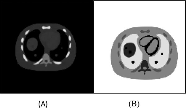
The CT (figure A) and PET (figure B) phantom used in the simulation. Five lesions are inserted into the lung and liver regions.
2.2 CT simulation
We used the Computer Assisted Tomography Simulator (CatSIM) (De Man et al. 2007) for the simulation of the X-ray CT imaging. The measurement model accounts for most system physical effects in CT scanners, including photon quantum noise, electronic noise, finite detector cell size, detector cross-talk, detector lag or afterglow, bowtie filtration, X-ray tube spectra, X-ray tube current, gantry rotation speed, and detector quantum efficiency.
A 140kVp polychromatic X-ray spectrum was used in our simulation. Let μ(ε) denote the energy (ε)-dependent attenuation distribution of a voxelized object of interest. Let Y denote the vector of CT measurements of the object μ(ε) with the element Yi denoting the ith measurement, where i = 1, ... , Nd and Nd is the number of measurements. The X-ray photons reaching the detector at each energy bin is modeled as a Poisson process and are converted to a signal proportional to the sum of energies. Electronic noise is modeled as Gaussian noise. Therefore the measurement Yi is a sum of the signal and noise, i.e.,
| (1) |
where fcon is a scalar factor to convert the x-ray energy from keV into the number of electrons, k is the energy bin index, and Ye is the independent Gaussian electronic noise modeled as . The mean number of absorbed photons Ȳι(εk) at energy εk is
| (2) |
where η(εk) denotes the detector quantum efficiency (fraction of photons absorbed), Ii(εk) denotes the number of photons arriving at the detector without attenuator for energy bin k, and l is the path length along the projection ray. Distance-Driven (DD) forward projection method (De Man & Basu 2004) is used for fast generation of the line integral for each projection ray.
We simulated an axial cone-beam CT geometry corresponding to the GE VCT 64 slice scanner. The longitudinal (z-) coverage of the detector was 40 mm. We included a quarter detector offset in the transaxial direction to reduce aliasing. We used a 140 kVp polychromatic spectrum produced by the XSPECT package (v3.5) in the simulation. The standard deviation of electronic noise was set to 5 photons (at 60 keV) per projection ray. We simulated four different ultra-low-dose levels in the study with integrated mA levels of 0.35 mAs, 0.175 mAs, 0.0875 mAs and 0.004375 mAs respectively. For each dose level, we simulated 7 different sparse view data acquisition protocols with view numbers starting from full view protocol of 984 views down to 8 views. The protocol and dose levels simulated are listed in Table 1. The baseline selected in the study is the simulation scan sampled at full view (984 view) and full dose (175 mAs). Two modes of data acquisition for sparse view data sampling are simulated: continuous exposure and tube pulsing. Continuous exposure mode was simulated by summarizing sub-views between neighboring views prior to log conversion. To simulate the tube pulsing data which is acquired by turning on the tube at desired location, we performed the simulation with all 984 views then dropped the views which are not needed. In this way, the exposure time for each view remains unchanged. In the tube pulsing data acquisition mode, the mA level is increased to maintain the equal dose level. For each protocol at each dose level, 20 independent and identical distributed (i.i.d.) noise realizations of CT scans are performed to assess the statistical variation for each data acquisition design.
Table 1.
Acquisition and reconstruction protocols for four total integrated tube current (mAs) levels.
| Dose Scheme | 0.35 mAs (Dose A), 0.175 mAs (Dose B), 0.0875 mAs (Dose C), 0.0475mAs (Dose D) |
| View numbers (sparse view sampling protocols) | 984 (protocol 1), 328 (protocol 2), 123(protocol 3), 41(protocol 4), 24(protocol 5), 12(protocol 6), 8(protocol 7) |
| Data acquisition mode | Continuous exposure, Tube Pulsing |
| Reconstruction mode | FDK without view interpolation, FDK with view interpolation, PWLS without view interpolation, PWLS with view interpolation |
2.3 CT image reconstruction
Since a polychromatic spectrum is used in the simulation, beam hardening correction is required. We performed a first-order beam hardening correction after the logarithm operation. With the presence of electronic noise, there can be negative values in the measurement, so a positivity mapping was applied to the data before the logarithm operation. All the negative values in the data were set to a small positive number ε.
| (3) |
where denotes the measurement of an air scan, denotes the measurement of an offset scan which is a scan without X-rays and without phantom.
Two types of reconstruction algorithms were performed for the sparse view data, conventional analytical FDK (Feldkamp et al. 1984), and penalized-weighted-least-square (PWLS) (Thibault et al. 2007, De Man and Fessler 2010).
The PWLS objective function has the form of
| (4) |
where μ is the vector of linear attenuation coefficients, A denotes the CT system matrix whose element aij denotes the contribution of the jth voxel to the ith measurement (De Man and Basu 2004, Long et al. 2010), wi ≈ Yi denote the statistical weighting (Fessler 1994, Thibault et al. 2007, Nuyts et al. 2013), and β is a scalar that controls the prior strength and hence the resolution and noise tradeoff. R(μ) is the penalty function which incorporates prior knowledge about the object, i.e.,
| (5) |
where μk denotes the neighbor voxel in the neighborhood Nj of the jth voxel. We selected a Markov random field Gibbs prior with a hyperbola potential function, whose parameter can be tuned to represent an approximate TV penalty. This has the form of
| (6) |
where δ controls the degree of edge preserving.
For very small values of δ, e.g., δ = 10−4/mm, the shape of hyperbola function is very close to that of the absolute value function, and the overall penalty R(μ) given in (5) becomes an approximation of the total-variation (TV) (Fessler 2006) potential function, which is commonly used in compressed sensing to exploit the sparsity in the gradient domain. The penalty strength β for the PWLS-TV was chosen to match the resolution of the standard kernel FDK reconstruction (Fessler and Rogers 1996). Figure 2 compares the β weighted penalty function of the PWLS-Hyperbola, PWLS-TV and absolute value function in the range of [−0.03, 0.03] /mm where first-order differences of voxels are included. We used β0 = 211 to scale the absolute value function so that the amplitude of β0 |t| matches that of the β-weighted penalty function of the PWLS-TV method. The β-weighted penalty function of the PWLS-TV method (green) overlaps with the scaled absolute value function (black). We used the ordered-subsets separable quadratic surrogates (OS-SQS) (Erdogân and Fessler 1999) algorithm to minimize the cost function ((4) of PWLS-TV method. To ensure the convergence of the PWLS-TV reconstructions, we used a large fixed number of iterations. For Protocols 1-3 we ran 40 OS iterations with 41 subsets followed by 360 regular iterations, and for Protocols 4-7 we ran 2000 regular iterations.
Figure 2.

The plot of three penalty functions: edge-preserving hyperbola (δ = 0. 02), approximate TV function (δ = 0. 0001) used in the study, and the absolute value function. We used β = 211 to scale the absolute value function so that the amplitude of β|t| matches the approximate TV function.
2.4 PET Simulations and Image Reconstruction
We simulated the 3D PET geometry of the GE Discovery 600 scanner, but used a single block ring consisting of 6 axial detectors resulting in 31 direct and oblique planes. The simulated system geometry has 339 radial bins, 256 angular bins, a FOV diameter of 700 mm and 40 mm longitudinal (z-) coverage per bed position. Let P denote the PET system matrix whose element pij models the probability that an even generated in the jth voxel is detected along the ith line- of-response (LOR). The system matrix can be factorized into two components to represent our model of the PET data acquisition process, i.e.,
| (7) |
where Patt is a diagonal matrix containing attenuation correction factors (ACFs) from CT images, and Pgeom models the geometrical mapping from the image space to the sinogram space based on generated by the distance-driven projector (De Man and Basu 2004, Manjeshwar et al. 2006).
Scatter was simulated using model based scatter estimation and was added to the analytical projection data (Iatrou, et al. 2006; Watson, et al. 1996, Ollinger, 1996). The resulting PET simulation data had 10 million counts including true and scattered coincidence events. Random coincidence events, detector blurring, and normalization were not modeled as our study focused on investigating the effects of attenuation correction with CT images on PET quantitation. 20 i.i.d. Poisson noise realizations of the PET sinogram data were generated.
A bilinear transformation was used to convert the CT reconstructed images to attenuation coefficients at 511 keV and used for PET reconstruction (Burger C. et al. 2002). Each of the 20 different PET noise realizations were reconstructed with each of the 20 sets of ACFs computed using standard bilinear interpolation from the CT images. As a result, each setting in Table 1 resulted in 400 separate PET images. PET images were reconstructed with 2 iterations, 28 subsets of OSEM (Hudson et al. 1994) using attenuation estimates from ultra-low dose CT. In keeping with common clinical protocols, PET images were generated with model based scatter estimation, and post-reconstruction 2D Gaussian filtering with a 6 mm FWHM and axial filter [1 6 1].
2.5 Evaluation Metrics
To quantify the quality of the PET reconstructed images, we selected evaluation metrics for global error and local PET quantitation error separately. The global ensemble root mean square error (RMSE) is used to represent the general image quality. Local PET lesion quantitation metrics include the ensemble bias and variances of the mean and max activity values at lesions across all the noise realizations.
The global ensemble RMSE is calculated as,
| (8) |
| (9) |
where RMSErp|rc is the RMSE of the rpth PET noise realization given the rcth CT noise realization with rc = 1, . . . , Rc and rp = 1, . . . , Rp , xrp|rc,j and x̂rp|rc,j denote the baseline (The baseline reference image we used the PET images with ACFS derived from FDK reconstructed full dose CT scan sampled with all views, which is a standard procedure in state-of-art PET/CT systems.) and simulation values at the jth voxel respectively, and N denotes the number of voxels within the region of interest (ROI) that covers the whole object.
To quantify the local PET lesion activity accuracy, we defined the error in lesion activity uptake (Errau) with respect to the baseline measurement as follows,
| (10) |
Where Nlesion denote the number of pixels in the lesion region. With randomness in both CT and PET simulations, we calculated the ensemble mean and variance of the Errau via expectation and total variance formulas:
| (11) |
| (12) |
3. Results
Results are obtained for four ultra-low-dose schemes (Dose A-0.35 mAs, Dose B-0.175 mAs, Dose C-0.0875 mAs, and Dose D-0.04375 mAs) for two data acquisition modes: continuous exposure and tube pulsing. For each dose scheme, 7 different protocols with different sampling views were simulated (Table 1).
Figure 3. shows the representative central slices of CT images with data acquired from tube pulsing technique at the dose level of 0.35 mAs for the 7 sampling protocols. Four methods are shown with a combination of analytic FDK versus PWLS-TV reconstruction and sparse view versus linear interpolation. For the FDK reconstruction (Figure 3.-a and -b), when there is a high number of angular samples each acquired with relatively low flux, the impact of the electronic noise starts to dominate the images. There is significant bias introduced as a result which can be seen for protocol 1 and 2. When the angular sampling decreases and X-ray flux per view increases, the relative effect of electronic noise reduces, thus decreasing the image noise and bias. However, when the angular sampling decreases further, the aliasing artifacts start to dominate image quality. With view interpolation the aliasing artifacts are reduced as shown in Figure 3.-b. However, the interpolation also introduced the azimuthal “swirling”-like smoothing onto the reconstructed images. PWLS-TV shows great advantage in terms of denosing and suppressing the aliasing artifacts compared to FDK as showing in Figure 3.-c and Figure 3.-d. There is still bias showing as dark shading on the images for protocol 1 and 2. When the angular sampling decreases, images with blocky texture are obtained (protocol 6 and 7). With PWLS-TV algorithm, when view interpolation is used, there are no obvious improvements. Moreover, the azimuthal smoothing introduced by the view interpolation introduces “swirling”-like smoothing artifact onto the images, as shown in Figure 3.-c and 3-d for protocols 5, 6 and 7.
Figure 3.

Central slices of CT images reconstructed with data acquired from tube pulsing technique at dose level A of 0.35 mAs. From left to right the images are listed according to the 7 protocols from full sampled 984 views down to 8 views. Figure (a) shows images reconstructed directly from sparse data using FDK reconstruction. Figure (b) shows images reconstructed from interpolated data using FDK reconstruction. Figure (c) shows images reconstructed directly from sparse data using PWLS-TV reconstruction. Figure (d) shows images reconstructed from interpolated data using PWLS-TV reconstruction.
Figure 4. shows the representative central slices of PET reconstruction images using the CT images shown in Figure 3 for attenuation correction. Using FDK reconstructed CT images directly from sparse sampled data, the bias and artifacts impacted the PET images. There are black shading regions and streaks on the PET images and the organs are not reconstructed correctly as shown in Figure 4.-a. Using FDK reconstructed CT images with view interpolation, the PET image improves visually as shown in Figure 4.-b. For protocol 1, 2 and 3, the PET images still have obvious bias. For protocol 6 and 7, the organs are smoothed azimuthally, and the shape of the organs is distorted. For sparse view sampling protocols 4 and 5, the PET images have visually good quality without obvious bias or artifacts. Using PWLS-TV greatly improved the visual PET images as shown in Figure 4.-c and Figure 4.-d.
Figure 4.

Corresponding central slices of PET reconstruction using CT images reconstructed in Figure 3 for attenuation correction. From left to right the images are listed according to the 7 protocols from full sampled 984 views down to 8 views. CT data are acquired from tube pulsing mode. From left to right is Protocol 1 to 7. Figure (a) shows images reconstructed directly from sparse data using FDK reconstruction. Figure (b) shows images reconstructed from interpolated data using FDK reconstruction. Figure (c) shows images reconstructed directly from sparse data using PWLS-TV reconstruction. Figure (d) shows images reconstructed from interpolated data using PWLS-TV reconstruction.
The representative central slices of CT reconstruction with data acquired from continuous exposure technique at dose level of 0.35 mAs and the corresponding PET reconstruction images are shown in Figure 5 and Figure 6. Continuous exposure data acquisition mode introduces blurring in the CT images, which is more pronounced as the view number reduces, as shown in Figure 5-a for FDK reconstruction with protocol 6 and 7. Similar impacts can be seen for PWLS-TV reconstruction with protocols 6 and 7, when compare to Figure 5-c to Figure 3-c.
Figure 5.

Central slices of CT images reconstructed with data acquired from continuous exposure technique at dose level A of 0.35 mAs. From left to right the images are listed according to the 7 protocols from full sampled 984 views down to 8 views. Figure (a) shows images reconstructed directly from sparse data using FDK reconstruction. Figure (b) shows images reconstructed from interpolated data using FDK reconstruction. Figure (c) shows images reconstructed directly from sparse data using PWLS-TV reconstruction. Figure (d) shows images reconstructed from interpolated data using PWLS-TV reconstruction.
Figure 6.

Corresponding central slices of PET reconstruction using CT images reconstructed in Figure 5 for attenuation correction. From left to right the images are listed according to the 7 protocols from full sampled 984 views down to 8 views. CT data are acquired from continuous exposure mode. From left to right is Protocol 1 to 7. Figure (a) shows images reconstructed directly from sparse data using FDK reconstruction. Figure (b) shows images reconstructed from interpolated data using FDK reconstruction. Figure (c) shows images reconstructed directly from sparse data using PWLS-TV reconstruction. Figure (d) shows images reconstructed from interpolated data using PWLS-TV reconstruction.
To quantitatively assess the image quality, the global ensemble RMSE and local lesion activity error were calculated. The ensemble RMSE is included in Table 2 for PET images with attenuation correction map provided by FDK reconstructed CT images with interpolation and PWLS-TV reconstructed CT images without interpolation for tube pulsing data acquisition mode. Any ensemble RMSE values of less than 3 × 10⁻³ are highlighted. When compare the images, PET images within this threshold still have visually good image quality and are free of significant artifacts. For FDK with interpolation, the ensemble RMSE value is within this range at dose A and dose B for sparse view protocols 4 and 5. With PWLS-TV reconstruction scheme, the ensemble RMSE for is improved compared to FDK reconstruction scheme at all four dose levels. The corresponding lesion activity error is included in Table 4. Protocols with an error less than 10% are highlighted in the table. The sparse view sampling improved the lesion activity error for all the five lesions. For FDK reconstruction with interpolation, at dose levels A and B, the lesion activity error for protocols 4 and 6 are all within 10% of the reference lesion activity. In addition to the improvement of ensemble RMSE, using PWLS-TV for CT reconstruction also improves the lesion quantitation. At dose level C, lesion activity errors are within 10% for protocols 4 and 5 for all five lesions. Even at dose D, lesion activity errors are still within 10 % for protocol 5 for all five lesions.
Table 2.
Ensemble RMSE of PET Images using ACFS from CT images reconstructed with FDK with Interpolation and PWLS without Interpolation for Tube Pulsing Technique
| FDK + Interpolation (× 10−3) | ||||
|---|---|---|---|---|
| Protocol | Dose A | Dose B | Dose C | Dose D |
| 1 | 660.5 ± 7.2 | 2139.9 ± 17.3 | 3885.3 ± 31.8 | 4293.5 ± 33.6 |
| 2 | 48.4 ± 0.6 | 285.1 ± 2.6 | 1297.5 ± 15.9 | 3492.8 ± 47.3 |
| 3 | 4.1 ± 0.2 | 20.5 ± 0.4 | 131.1 ± 2.3 | 714.1 ± 11.7 |
| 4 | 2.4 ± 0.4 | 2.8 ± 0.3 | 6.6 ± 0.2 | 39.7 ± 0.7 |
| 5 | 2.6 ± 0.3 | 2.7 ± 0.3 | 3.3 ± 0.2 | 8.9 ± 0.2 |
| 6 | 3.3 ± 0.2 | 3.3 ± 0.2 | 3.3 ± 0.2 | 3.8 ± 0.2 |
| 7 | 3.6 ± 0.2 | 3.6 ± 0.2 | 3.6 ± 0.2 | 3.9 ± 0.2 |
| PWLS-TV (× 10−3) | ||||
|---|---|---|---|---|
| Protocol | Dose A | Dose B | Dose C | Dose D |
| 1 | 4.5 ± 0.1 | 5.5 ± 0.06 | 6.3 ± 0.04 | 7.0 ± 0.02 |
| 2 | 3.0 ± 0.2 | 3.9 ± 0.1 | 4.9 ± 0.1 | 5.8 ± 0.5 |
| 3 | 2.5 ± 0.3 | 2.8 ± 0.2 | 3.5 ± 0.2 | 4.5 ± 0.1 |
| 4 | 2.4 ± 0,3 | 2.4 ± 0.3 | 2.6 ± 0.3 | 3.0 ± 0.2 |
| 5 | 2.4 ± 0.3 | 2.4 ± 0.3 | 2.5 ± 0.3 | 2.7 ± 0.2 |
| 6 | 2.8 ± 0.2 | 2.8 ± 0.2 | 2.9 ± 0.2 | 3.0 ± 0.2 |
| 7 | 3.4 ± 0.2 | 3.4 ± 0.2 | 3.4 ± 0.2 | 3.5 ± 0.2 |
Table 4.
PET Lesion Activity Error using ACFS from CT images reconstructed with FDK with Interpolation and PWLS without Interpolation for Tube Pulsing Technique
| Lesion 1: 10 mm liver lesion | |||||||||
|---|---|---|---|---|---|---|---|---|---|
| FDK + Interpolation |
PWLS-TV |
||||||||
| Pro | Dose A | Dose B | Dose C | Dose D | Pro | Dose A | Dose B | Dose C | Dose D |
| 1 (× 104) | 0.3 ± 0.02 | 1.2 ± 0.07 | 2.8 ± 0.1 | 3.7 ± 0.3 | 1 | –34.5 ± 0.5 | 49.9 ± 0.5 | –63.0 ± 0.4 | –73.5 ± 0.3 |
| 2 (× 103) | 0.2 ± 0.01 | 1.2 ± 0.9 | 5.8 ± 0.4 | 19.6 ± 2.0 | 2 | –14.5 ± 0.4 | –25.7 ± 0.5 | –40.9 ± 0.5 | –55.6 ± 0.5 |
| 3 (× 102) | 0.2 ± 0.02 | 1.0 ± 0.09 | 5.0 ± 0.4 | 25.8 ± 2.9 | 3 | –6.9 ± 0.3 | –11.3 ± 0.4 | –20.6 ± 0.5 | –34.4 ± 0.6 |
| 4 | 3.6 ± 0.5 | 8.0 ± 1.1 | 32.0 ± 3.6 | 183.0 ± 15.1 | 4 | –4.5 ± 0.2 | –5.5 ± 0.3 | –8.2 ± 0.4 | –14.3 ± 0.5 |
| 5 | 1.8 ± 0.4 | 3.0 ± 0.5 | 9.0 ± 1.3 | 47.0 ± 4.0 | 5 | –3.8 ± 0.2 | –4.4 ± 0.3 | –5.5 ± 0.4 | –8.8 ± 0.6 |
| 6 | –5.2 ± 0.5 | –5.0 ± 0.6 | –4.0 ± 0.6 | –1.0 ± 0.9 | 6 | –7.4 ± 0.3 | –7.7 ± 0.4 | –8.0 ± 0.5 | –10.0 ± 0.7 |
| 7 | 18.1 ± 0.7 | –18.0 ± 0.7 | –18.0 ± 0.7 | –18.0 ± 0.7 | 7 | –7.8 ± 0.5 | –7.9 ± 0.6 | –8.4 ± 0.8 | –10.4 ± 0.7 |
| Lesion 2: 15 mm liver lesion | |||||||||
|---|---|---|---|---|---|---|---|---|---|
| FDK + Interpolation |
PWLS-TV |
||||||||
| Pro | Dose A | Dose B | Dose C | Dose D | Pro | Dose A | Dose B | Dose C | Dose D |
| 1 (× 104) | 0.2 ± 0.01 | 0.6 ± 0.05 | 1.8 ± 0.1 | 2.9 ± 0.1 | 1 | –34.5 ± 0.3 | –49.5 ± 0.3 | –62.4 ± 0.2 | –73.2 ± 0.2 |
| 2 (× 103) | 0.03 ± 0.01 | 1.1 ± 0.05 | 3.9 ± 0.3 | 13.3 ± 1.4 | 2 | –15.0 ± 0.2 | –26.2 ± 0.3 | –40.8 ± 0.3 | –55.4 ± 0.3 |
| 3 (× 102) | 0.2 ± 0.01 | 1.2 ± 0.07 | 5.6 ± 0.4 | 19.8 ± 1.9 | 3 | –7.3 ± 0.2 | –11.8 ± 0.2 | –20.9 ± 0.3 | –34.7 ± 0.3 |
| 4 | 2.6 ± 0.3 | 6.5 ± 0.5 | 35.0 ± 3.8 | 211.0 ± 13.3 | 4 | –5.2 ± 0.2 | –6.2 ± 0.2 | –8.9 ± 0.3 | –15.1 ± 0.4 |
| 5 | 3.9 ± 0.2 | 4.8 ± 0.4 | 10.0 ± 1.4 | 59.0 ± 4.7 | 5 | –4.8 ± 0.1 | –5.2 ± 0.2 | –6.4 ± 0.2 | –9.7 ± 0.3 |
| 6 | 0.0 ± 0.3 | 2.0 ± 0.3 | 1.0 ± 0.4 | 5.0 ± 0.8 | 6 | 0.5 ± 0.2 | 0.3 ± 0.3 | –0.4 ± 0.4 | –2.2 ± 0.9 |
| 7 | –6.3 ± 0.3 | –6.2 ± 0.3 | –6.0 ± 0.4 | –6.0 ± 0.4 | 7 | –10.75 ± 0.4 | –11.0 ± 0.4 | –11.0 ± 0.5 | –11.6 ± 0.6 |
| Lesion 3: 15 mm right lung lesion | |||||||||
|---|---|---|---|---|---|---|---|---|---|
| FDK + Interpolation |
PWLS-TV |
||||||||
| Pro | Dose A | Dose B | Dose C | Dose D | Pro | Dose A | Dose B | Dose C | Dose D |
| 1 (× 103) | 0.2 ± 0.03 | 0.02 ± 0.09 | 2.0 ± 0.5 | 13.2 ± 1.0 | 1 | –16.7 ± 0.2 | –30.3 ± 0.2 | –45.6 ± 0.2 | –60.1 ± 0.2 |
| 2 (× 102) | 0.1 ± 0.07 | 1.4 ± 0.3 | 3.4 ± 0.9 | 9.7 ± 4.1 | 2 | –5.8 ± 0.2 | –10.9 ± 0.3 | –21.8 ± 0.4 | –36.7 ± 0.3 |
| 3 | –1.4 ± 1.0 | 5.5 ± 5.1 | 58.2 ± 23.8 | 230.0 ± 62.3 | 3 | –4.8 ± 0.1 | –5.2 ± 0.2 | –8.1 ± 0.3 | –16.8 ± 0.4 |
| 4 | –2.0 ± 0.4 | –5.0 ± 0.7 | –4.6 ± 3.4 | 10.0 ± 11.0 | 4 | –5.6 ± 0.3 | –5.6 ± 0.2 | –5.7 ± 0.3 | –6.8 ± 0.6 |
| 5 | –3.1 ± 0.3 | –4.5 ± 0.5 | –7.8 ± 1.7 | –4.0 ± 4.0 | 5 | –8.8 ± 0.3 | –8.8 ± 0.3 | –9.1 ± 0.4 | –9.0 ± 0.6 |
| 6 | –2.1 ± 0.4 | –2.1 ± 0.4 | –3.2 ± 0.6 | –9.0 ± 1.4 | 6 | –9.8 ± 0.4 | –9.7 ± 0.4 | –9.7 ± 0.6 | –9.0 ± 0.6 |
| 7 | –12.1 ± 0.6 | –12.2 ± 0.6 | –12.7 ± 0.7 | –17.0 ± 1.1 | 7 | –2.8 ± 0.5 | –2.8 ± 0.5 | –2.7 ± 0.7 | –3.4 ± 0.8 |
| Lesion 4: 10 mm right lung lesion | |||||||||
|---|---|---|---|---|---|---|---|---|---|
| FDK + Interpolation |
PWLS-TV |
||||||||
| Pro | Dose A | Dose B | Dose C | Dose D | Pro | Dose A | Dose B | Dose C | Dose D |
| 1 | –66.8 ± 10.7 | –95.2 ± 3.8 | –73.5 ± 21.7 | 3925.4 ± 15.2 | 1 | –12.0 ± 0.6 | –22.1 ± 0.7 | –36.3 ± 0.7 | –51.8 ± 0.6 |
| 2 | 9.6 ± 10.4 | 14.7 ± 17.7 | –54.6 ± 34.1 | –64.5 ± 43.0 | 2 | –6.0 ± 0.4 | –8.6 ± 0.5 | –15.5 ± 0.7 | –27.8 ± 0.8 |
| 3 | –4.1 ± 1.2 | –7.0 ± 5.9 | 8.0 ± 15.4 | –47.1 ± 22.7 | 3 | –5.4 ± 0.3 | –5.6 ± 0.4 | –6.9 ± 0.6 | –12.1 ± 0.8 |
| 4 | –1.6 ± 0.3 | –3.7 ± 0.7 | –12.1 ± 2.8 | –17.6 ± 9.0 | 4 | –5.6 ± 0.3 | –5.6 ± 0.4 | –5.3 ± 0.5 | –5.7 ± 0.7 |
| 5 | –4.5 ± 0.5 | –5.4 ± 0.6 | –9.0 ± 0.9 | –20.0 ± 4.0 | 5 | –7.9 ± 0.5 | –7.8 ± 0.5 | –7.5 ± 0.6 | –6.7 ± 1.1 |
| 6 | –1.2 ± 0.5 | –1.2 ± 0.5 | –1.7 ± 0.6 | –4.0 ± 1.1 | 6 | –12.0 ± 0.8 | –12.1 ± 0.7 | –11.8 ± 0.8 | –11.0 ± 0.9 |
| 7 | 6.9 ± 0.7 | 6.9 ± 0.7 | 6.9 ± 0.8 | 4.9 ± 0.9 | 7 | –21.7 ± 1.1 | –21.7 ± 1.2 | –21.5 ± 1.2 | –20.8 ± 1.5 |
| Lesion 5: 15 mm left lung lesion | |||||||||
|---|---|---|---|---|---|---|---|---|---|
| FDK + Interpolation |
PWLS-TV |
||||||||
| Pro | Dose A | Dose B | Dose C | Dose D | Pro | Dose A | Dose B | Dose C | Dose D |
| 1 (× 104) | 0.03 ± 0.01 | 0.3 ± 0.03 | 1.1 ± 0.1 | 2.7 ± 0.2 | 1 | –15.7 ± 0.3 | –30.8 ± 0.3 | –46.2 ± 0.3 | –60.6 ± 0.3 |
| 2 (× 103) | –0.01 ± 0.01 | 0.09 ± 0.04 | 1.4 ± 0.2 | 8.3 ± 1.0 | 2 | –4.1 ± 0.2 | –9.4 ± 0.3 | –21.4 ± 0.4 | –37.2 ± 0.4 |
| 3 | –4.1 ± 1.2 | –4.0 ± 5.8 | 2.0 ± 20.7 | 678.0 ± 153.1 | 3 | –3.9 ± 0.2 | –3.6 ± 0.3 | –6.3 ± 0.4 | –15.8 ± 0.5 |
| 4 | –4.0 ± 0.3 | –6.7 ± 0.7 | –10.0 ± 2.9 | –31.0 ± 8.3 | 4 | –4.8 ± 0.2 | –4.7 ± 0.3 | –4.2 ± 0.4 | –4.7 ± 0.6 |
| 5 | –9.1 ± 0.4 | –11.2 ± 0.5 | –15.0 ± 1.6 | –10.0 ± 3.2 | 5 | –7.4 ± 0.2 | –7.2 ± 0.3 | –7.1 ± 0.4 | –6.6 ± 0.6 |
| 6 | –3.6 ± 0.4 | –3.6 ± 0.4 | –5.0 ± 0.6 | –9.0 ± 1.0 | 6 | –12.0 ± 0.4 | –11.2 ± 0.5 | –11.8 ± 0.6 | –11.2 ± 0.6 |
| 7 | 4.5 ± 0.4 | 4.6 ± 0.5 | 5.0 ± 0.5 | 5.0 ± 0.9 | 7 | –8.2 ± 0.4 | –8.2 ± 0.4 | –8.5 ± 0.5 | –9.7 ± 0.8 |
The ensemble RMSE and lesion activity error for PET images reconstructed with CT data acquired using continuous exposure technique are listed in Table 5 and Table 3. The quantitative results for continuous exposure data acquisition are slightly worse compared to tube pulsing using the same CT reconstruction scheme. With CT images reconstructed by FDK with interpolation, the lesion activity error and ensemble RMSE for sparse sampling protocols 4 and 5 are similar between the two data acquisition modes for dose levels A and B. For dose levels C and D, the corresponding ensemble RMSE and lesion activity error increases slightly compared to the tube pulsing technique. Using PWLS-TV for CT image reconstruction, the ensemble RMSE error for protocols 4 and 5 are comparable between the two data acquisition modes. However, for lesion activity error, at dose D, no protocol can provide lesion quantitation error within 10% anymore.
Table 5.
PET Lesion Activity Error using ACFS from CT images reconstructed with FDK with Interpolation and PWLS without Interpolation for Continuous exposure Technique
| Lesion 1: 10 mm liver lesion | |||||||||
|---|---|---|---|---|---|---|---|---|---|
| FDK + Interpolation |
PWLS-TV |
||||||||
| Pro | Dose A | Dose B | Dose C | Dose D | Pro | Dose A | Dose B | Dose C | Dose D |
| 1 (× 104) | 0.3 ± 0.01 | 1.2 ± 0.05 | 2.7 ± 0.1 | 3.9 ± 0.5 | 1 | –34.4 ± 0.5 | –50.0 ± 0.5 | –63.1 ± 0.4 | –73.5 ± 0.4 |
| 2 (× 103) | 0.2 ± 0.01 | 1.2 ± 0.1 | 5.8 ± 0.3 | 19.7 ± 2.4 | 2 | –14.5 ± 0.4 | –25.8 ± 0.5 | –40.9 ± 0.5 | –55.8 ± 0.5 |
| 3 (× 102) | 0.1 ± 0.01 | 1.0 ± 0.07 | 5.3 ± 0.5 | 25.0 ± 1.2 | 3 | –7.0 ± 0.3 | –11.3 ± 0.3 | –20.7 ± 0.5 | –33.9 ± 0.5 |
| 4 | 2.3 ± 0.3 | 6.0 ± 0.8 | 27.0 ± 2.4 | 162.0 ± 9.5 | 4 | –4.8 ± 0.2 | –5.9 ± 0.3 | –8.6 ± 0.3 | –14.7 ± 0.5 |
| 5 | –0.6 ± 0.4 | 0.0 ± 0.5 | 4.0 ± 1.4 | 35.0 ± 2.7 | 5 | –4.9 ± 0.3 | –5.3 ± 0.4 | –6.7 ± 0.4 | –9.5 ± 0.4 |
| 6 | –14.9 ± 0.6 | –15.0 ± 0.7 | –14.0 ± 0.7 | –14.0 ± 0.7 | 6 | –12.5 ± 0.6 | –12.8 ± 0.6 | –13.5 ± 0.8 | –14.1 ± 1.0 |
| 7 | –25.4 ± 0.8 | –25.0 ± 0.8 | –25.0 ± 0.8 | –25.0 ± 0.9 | 7 | –21.0 ± 0.8 | –21.0 ± 0.8 | –21.5 ± 1.1 | –22.7 ± 0.8 |
| Lesion 2: 15 mm liver lesion | |||||||||
|---|---|---|---|---|---|---|---|---|---|
| FDK + Interpolation |
PWLS-TV |
||||||||
| Pro | Dose A | Dose B | Dose C | Dose D | Pro | Dose A | Dose B | Dose C | Dose D |
| 1 (× 104) | 0.2 ± 0.01 | 0.6 ± 0.04 | 1.9 ± 0.1 | 2.9 ± 0.09 | 1 | –34.4 ± 0.3 | –49.6 ± 0.3 | –62.5 ± 0.2 | –73.1 ± 0.2 |
| 2 (× 103) | 0.3 ± 0.01 | 1.1 ± 0.06 | 3.9 ± 0.3 | 12.6 ± 0.6 | 2 | –14.9 ± 0.2 | –26.2 ± 0.3 | –40.8 ± 0.3 | –55.4 ± 0.3 |
| 3 (× 102) | 0.1 ± 0.01 | 1.2 ± 0.03 | 5.6 ± 2.3 | 19.6 ± 1.0 | 3 | –7.3 ± 0.2 | –12.0 ± 0.2 | –20.9 ± 0.2 | –34.8 ± 0.3 |
| 4 | 2.0 ± 0.2 | 4.3 ± 0.6 | 29.0 ± 0.4 | 199.0 ± 12.0 | 4 | –5.0 ± 0.1 | –6.0 ± 0.2 | –8.8 ± 0.3 | –15.1 ± 0.4 |
| 5 | 1.0 ± 0.2 | 1.8 ± 0.3 | 5.0 ± 0.9 | 37.0 ± 4.2 | 5 | –4.4 ± 0.1 | –4.8 ± 0.2 | –6.1 ± 0.2 | –8.9 ± 0.2 |
| 6 | –8.2 ± 0.3 | –7.9 ± 0.3 | 7.0 ± 0.4 | –6.0 ± 0.4 | 6 | –5.8 ± 0.3 | –6.0 ± 0.3 | –6.4 ± 0.3 | –7.2 ± 0.4 |
| 7 | –14.8 ± 0..4 | –14.7 ± 0.4 | –15.0 ± 0.4 | –14.0 ± 0.4 | 7 | –14.6 ± 0. | –14.6 ± 0.3 | –14.9 ± 0.5 | –15.3 ± 0.5 |
| Lesion 3: 15 mm right lung lesion | |||||||||
|---|---|---|---|---|---|---|---|---|---|
| FDK + Interpolation |
PWLS-TV |
||||||||
| Pro | Dose A | Dose B | Dose C | Dose D | Pro | Dose A | Dose B | Dose C | Dose D |
| 1 (× 103) | 0.1 ± 0.03 | 0.3 ± 0.06 | 1.8 ± 0.4 | 15.1 ± 1.4 | 1 | –16.5 ± 0.2 | –30.3 ± 0.2 | –45.6 ± 0.2 | –60.0 ± 0.2 |
| 2 (× 102) | 0.1 ± 0.09 | 1.2 ± 0.2 | 3.4 ± 0.9 | 7.0 ± 3.0 | 2 | –5.8 ± 0.2 | –10.9 ± 0.3 | –22.0 ± 0.2 | –37.0 ± 0.3 |
| 3 | –2.1 ± 0.7 | 3.9 ± 5.9 | 65.3 ± 8.7 | 232.0 ± 24.3 | 3 | –5.0 ± 0.1 | –5.2 ± 0.3 | –8.5 ± 0.3 | –17.0 ± 0.6 |
| 4 | –3.9 ± 0.2 | –7.0 ± 0.5 | –11.4 ± 1.6 | –9.0 ± 11.0 | 4 | –7.4 ± 0.2 | –7.4 ± 0.2 | –7.3 ± 0.2 | –8.1 ± 0.4 |
| 5 | –8.1 ± 0.3 | –8.7 ± 0.3 | –13.4 ± 0.5 | –27.0 ± 1.6 | 5 | –12.5 ± 0.3 | –12.2 ± 0.5 | –12.4 ± 0.4 | –12.7 ± 0.5 |
| 6 | –6.3 ± 0.4 | –6.2 ± 0.5 | –6.2 ± 0.4 | –8.0 ± 0.8 | 6 | –15.7 ± 0.4 | –15.6 ± 0.5 | –15.7 ± 0.4 | –15.2 ± 0.5 |
| 7 | –8.0 ± 0.4 | –8.0 ± 0.4 | –8.0 ± 0.4 | –8.0 ± 0.6 | 7 | –6.5 ± 0.4 | –6.4 ± 0.4 | –6.7 ± 0.4 | –7.0 ± 0.4 |
| Lesion 4: 10 mm right lung lesion | |||||||||
|---|---|---|---|---|---|---|---|---|---|
| FDK + Interpolation |
PWLS-TV |
||||||||
| Pro | Dose A | Dose B | Dose C | Dose D | Pro | Dose A | Dose B | Dose C | Dose D |
| 1 | –57.2 ± 15.7 | –93.4 ± 4.8 | 18.3 ± 81.9 | 3033.7 ± 752.7 | 1 | –12.0 ± 0.6 | –22.1 ± 0.7 | –36.2 ± 0.7 | –52.8 ± 0.6 |
| 2 | 10.2 ± 6.9 | 38.5 ± 22.0 | –60.6 ± 22.7 | –61.5 ± 26.3 | 2 | –5.7 ± 0.3 | –8.5 ± 0.5 | –15.5 ± 0.6 | –27.4 ± 0.8 |
| 3 | –4.6 ± 1.4 | –13.8 ± 3.1 | 6.0 ± 7.5 | –55.7 ± 28.2 | 3 | –5.5 ± 0.2 | –5.6 ± 0.4 | –7.3 ± 0.8 | –12.2 ± 0.6 |
| 4 | –4.5 ± 0.4 | –5.9 ± 0.6 | –14.2 ± 1.8 | 42.7 ± 6.0 | 4 | –7.9 ± 0.3 | –7.8 ± 0.5 | –7.4 ± 0.5 | –7.8 ± 0.8 |
| 5 | –8.2 ± 0.5 | –8.5 ± 0.5 | –10.6 ± 0.8 | –23.6 ± 2.9 | 5 | –14.6 ± 0.6 | –12.1 ± 0.7 | –14.2 ± 0.6 | –13.0 ± 0.7 |
| 6 | –7.1 ± 0.7 | –7.0 ± 0.7 | –6.8 ± 0.7 | –8.0 ± 0.8 | 6 | –14.0 ± 0.7 | –14.0 ± 0.8 | –13.7 ± 0.8 | –13.0 ± 0.7 |
| 7 | –2.7 ± 0.7 | –2.7 ± 0.7 | –2.5 ± 0.7 | –2.7 ± 0.8 | 7 | –23.4 ± 1.3 | –23.2 ± 1.4 | –23.1 ± 1.3 | –23.2 ± 1.6 |
| Lesion 5: 15 mm left lung lesion | |||||||||
|---|---|---|---|---|---|---|---|---|---|
| FDK + Interpolation |
PWLS-TV |
||||||||
| Pro | Dose A | Dose B | Dose C | Dose D | Pro | Dose A | Dose B | Dose C | Dose D |
| 1 (× 104) | 0.04 ± 0.01 | 0.3 ± 0.02 | 1.1 ± 0.1 | 2.7 ± 0.2 | 1 | –15.7 ± 0.3 | –30.7 ± 0.3 | –46.1 ± 0.3 | –60.7 ± 0.2 |
| 2 (× 103) | –0.02 ± 0.01 | 0.07 ± 0.01 | 1.3 ± 0.1 | 8.0 ± 1.5 | 2 | –4.1 ± 0.2 | –9.2 ± 0.4 | –21.5 ± 0.4 | –37.5 ± 0.3 |
| 3 | –3.8 ± 1.6 | –4.1 ± 3.5 | –16.0 ± 15.9 | 495.0 ± 197.9 | 3 | –4.2 ± 0.2 | –3.9 ± 0.3 | 6.5 ± 0.3 | –16.0 ± 0.4 |
| 4 | –4.8 ± 0.3 | –8.1 ± 0.5 | –14.0 ± 1.0 | –33.0 ± 4.7 | 4 | –6.6 ± 0.2 | –6.4 ± 0.2 | –5.9 ± 0.2 | –6.2 ± 0.5 |
| 5 | –8.0 ± 0.3 | –9.0 ± 0.5 | –13.0 ± 0.9 | –18.0 ± 1.8 | 5 | –9.9 ± 0.3 | –9.5 ± 0.3 | –9.0 ± 0.3 | –9.0 ± 0.3 |
| 6 | 1.6 ± 0.3 | 1.8 ± 0.4 | 2.0 ± 0.4 | 0.0 ± 1.1 | 6 | –10.1 ± 0.3 | –10.2 ± 0.6 | –10.0 ± 0.4 | –9.5 ± 0.8 |
| 7 | 10.5 ± 0.4 | 10.5 ± 0.4 | 11.0 ± 0.4 | 11.0 ± 0.5 | 7 | 0.9 ± 0.4 | 0.7 ± 0.5 | 0.7 ± 0.4 | 0.5 ± 0.5 |
Table 3.
Ensemble RMSE of PET Images fusing ACFS from CT images reconstructed with FDK with Interpolation and PWLS without Interpolation for Continuous exposure Technique
| FDK + Interpolation (× 10−3) | ||||
|---|---|---|---|---|
| Protocol | Dose A | Dose B | Dose C | Dose D |
| 1 | 660.6 ± 5.3 | 2138.3 ± 12.9 | 3873.7 ± 20.6 | 4307.2 ± 16.7 |
| 2 | 48.5 ± 0.4 | 284.0 ± 2.1 | 1296.1 ± 9.1 | 3480.1 ± 17.0 |
| 3 | 4.0 ± 0.2 | 20.1 ± 0.3 | 130.3 ± 1.5 | 711.4 ± 12.1 |
| 4 | 2.4 ± 0.4 | 2.7 ± 0.3 | 5.8 ± 0.2 | 35.2 ± 1.3 |
| 5 | 2.7 ± 0.3 | 2.7 ± 0.3 | 3.0 ± 0.2 | 6.6 ± 0.1 |
| 6 | 3.3 ± 0.2 | 3.3 ± 0.2 | 3.3 ± 0.2 | 3.3 ± 0.2 |
| 7 | 3.8 ± 0.2 | 3.8 ± 0.2 | 3.8 ± 0.2 | 3.8 ± 0.2 |
| PWLS-TV (× 10−3) | ||||
|---|---|---|---|---|
| Protocol | Dose A | Dose B | Dose C | Dose D |
| 1 | 4.5 ± 0.1 | 5.5 ± 0.1 | 6.3 ± 0.04 | 7.0 ± 0.02 |
| 2 | 3.0 ± 0.2 | 3.9 ± 0.1 | 4.9 ± 0.1 | 5.8 ± 0.05 |
| 3 | 2.5 ± 0.3 | 2.8 ± 0.2 | 3.5 ± 0.1 | 4.5 ± 0.1 |
| 4 | 2.5 ± 0.3 | 2.5 ± 0.3 | 2.7 ± 0.2 | 3.1 ± 0.2 |
| 5 | 2.6 ± 0.3 | 2.7 ± 0.3 | 2.7 ± 0.2 | 2.9 ± 0.2 |
| 6 | 3.3 ± 0.2 | 3.3 ± 0.2 | 3.3 ± 0.2 | 3.4 ± 0.2 |
| 7 | 4.0 ± 0.1 | 4.0 ± 0.1 | 4.0 ± 0.1 | 4.0 ± 0.1 |
For each data acquisition and image reconstruction method, we selected the optimal protocol based on visual PET image quality, and both quantitative analysis results for ensemble RMSE and lesion activity error. The images for selected optimal protocol at each dose level are shown in Figure 7. For FDK reconstruction CT images with interpolation, protocol 4 was selected and the images for each dose scheme are shown in Figure 7-a and -b for tube pulsing and continuous exposure techniques. For dose levels C and D, noise and/or streaking artifacts become more prevalent across view protocols. For PWLS reconstruction, we select protocol 5 without view interpolation and show the images for each dose scheme in Figure 7-c and -d for tube pulsing and continuous exposure techniques. Corresponding PET reconstructed images are shown in Figure 8.
Figure 7.

Representative central slices of reconstructed CT images for selected protocols. From left to right are the CT reconstruction images at full dose for reference (R), 0.35mAs (A), 0.175 mAs (B), 0.0875mAs (C), and 0.04375mAs (D). Figure (a) is FDK reconstruction with view interpolation for protocol 4 for tube pulsing data acquisition. Figure (b) is FDK reconstruction with view interpolation for protocol 4 for continuous exposure data acquisition. Figure (c) is PWLS reconstruction without view interpolation for protocol 5 for tube pulsing data acquisition. Figure (d) is PWLS reconstruction with view interpolation for protocol 5 for continuous exposure data acquisition.
Figure 8.

Corresponding central slices of PET reconstruction using CT images reconstructed in Figure 7. for attenuation correction. From left to right are PET images reconstructed using the CT reconstruction images at full dose for reference (R), 0.35mAs (A), 0.175 mAs(B), 0.0875mAs(C), and 0.04375mAs(D). Figure (a) uses FDK reconstructed CT images with view interpolation for protocol 4 for tube pulsing data acquisition. Figure (b) uses FDK reconstructed CT images with view interpolation for protocol 4 for continuous exposure data acquisition. Figure (c) uses PWLS reconstructed CT images without view interpolation for protocol 5 for tube pulsing data acquisition. Figure (d) uses PWLS reconstructed CT images with view interpolation for protocol 5 for continuous exposure data acquisition.
The PET images reconstructed using ACFs from CT images reconstructed using FDK without view interpolation have significant noise and artifacts. The quantitative analysis of these images shows increased lesion activity error and ensemble RMSE. Using PWLS-TV with view interpolation for the CT reconstruction did not improve the visual PET image quality, but rather introduce “swirling” smoothing artifacts when the view number was low. Quantitative analysis for this set of images also shows no improvement for lesion activity error or ensemble RMSE (data not shown).
4. Discussion
In this study, we aim to reduce the CT scan dose below the conventional electronic noise barrier limits using sparse view data acquisition. In sparse view data acquisition, instead of delivering dose to many views the same amount of dose is delivered to a limited number of sampling points. In this case, the signal to noise ratio for each measurement can be improved for same electronic noise level. However, with reduced view sampling, aliasing artifacts can result in image bias. When CT images are used for attenuation correction (CTAC), these errors propagate to PET images (Kinahan et al. , 2006) affecting lesion detection and quantitation. At ultra-low dose levels (≤ 0.35 mAs as we simulated in the study), sparse view sampling can reduce the noise and bias of CT images and therefore improve the corresponding PET image quality. With protocols 1 and 2, electronic noise in the measurements causes high noise and bias in the PET images. For protocols 6 and 7, there are not enough measurements for an accurate CT image reconstruction and the resulting PET images have poor good image quality. Sparse view sampling protocols 4 and 5 balance the electronic noise and aliasing artifacts. Quantitative analysis for the lesion activity error and global ensemble RMSE in PET images also indicated an improvement by using sparse view sampling. The optimal number of view sampling depends on the dose level, data acquisition mode and the reconstruction scheme, which should be tuned for a specific system.
MBIR shows a further advantage over FDK in reconstructing images at ultra-low dose and with sparse sampling. In this study, we selected a PWLS-TV cost function and optimize it using the OS-SQS algorithm. For protocols 1 and 2 PWLS-TV reduced the global ensemble RMSE by over a factor of 100 compared to FDK reconstruction for PET images, regardless of the data acquisition mode.. Even at dose level C, using PWLS-TV reconstruction, for protocol 5, the organs and lesions in the phantom are reconstructed properly with clear boundaries and correct shape for CT (Figure 5) and the corresponding PET images (Figure 6).
The ideal sparse data acquisition mode is to pulse the X-ray tube. This requires the hardware to switch the X-ray tube on and off frequently within one short rotation (0.35 second in our simulation). A continuous exposure technique does not require tube pulsing hardware and simply allows the X-ray tube to be on during the entire data acquisition time. This will introduce azimuthal blur due to the integration of the signal. For CT-based attenuation correction (CTAC), the incremental azimuthal blur introduced by continuous exposure data acquisition did not measurably impact the PET image quality. This study suggests, for protocols 4 and 5 (41 and 24 views), the impact of this blur can be neglected. The overall PET image quality and quantitative measurements are in general comparable between the two data acquisition modes for dose levels A and B despite the reconstruction scheme. When we further reduce the dose, the lesion activity error increases more with continuous exposure data acquisition than with tube pulsing. Continuous exposure data acquisition can be implemented on today's PET/CT system without hardware upgrade, so its cost of implementation is potentially much lower. Since tube pulsing offers only a minor performance gain, continuous exposure technique is an attractive candidate for practical sparse sampling data acquisition.
View interpolation can be used to fill the missing information caused by sparse sampling. For FDK CT reconstruction, view interpolation is essential for sparsely sampled sinogram. Aliasing artifacts due to the missing angular sampling are significantly reduced with view interpolation. As a result, PET visual image quality and quantitative assessment improve accordingly. View interpolation is not necessary for MBIR, and in fact can be detrimental. With few views, the smoothing introduced by interpolation results in a “swirling” artifacts on CT images that degrade the PET image quality.
We evaluated the PET image quality measuring local lesion activity error and global ensemble RMSE. We inserted five lesions at different locations of the phantom, two in the liver, and three in the lung. The local lesion activity highly depends on the location of the lesion, and it is possible that the performance of this local metric may not align with the overall image quality. For example, the combination of sampling protocol 6 + FDK + view interpolation reconstruction scheme had good local lesion quantitation for tube pulsing data acquisition as highlighted in Table 4. However, the CT images have “swirling” artifacts and the corresponding PET images inherited this artifact (Figure 3-b and Figure 4-b). The ensemble RMSE was also increased for this protocol (Table 2). It is possible that for this sampling protocol, the sampling position coincidently aligns with the lesion locations; therefore, the local lesion activity is well reconstructed. The same is true for the other sparse sampling protocols; lesions at certain locations can be well reconstructed despite the poor overall image quality. Therefore, the local lesion accuracy metric should be combined with the global and qualitative metrics to determine the PET image quality. The baseline references used in the comparison are PET images attenuation-corrected with CT FDK reconstructed images, which in turn are sampled with full number of views and with a high radiation dose. With high dose and sufficient sampling, the CT images reconstructed by FDK and iterative algorithms are essentially identical for the purpose of this study: neither has any significant noise or aliasing artifact. We could have used the CT images reconstructed by iterative algorithms for consistency; however, FDK reconstruction was chosen as baseline since it is the industry standard.
For a specific system, the lowest dose and optimal view sampling protocol might differ given configurations of the system. In this study, we selected a Gaussian model to represent the behavior of electronic noise, although this may not be accurate in real systems (Zabic et al. 2013). More advanced algorithms, such as boxcar CT sinogram smoothing followed by adaptive trimmed mean filter (Hsieh 1998, Colsher et al. 2008), could be helpful in reducing PET bias and noise (Xia et al. 2012). The statistical model in most iterative reconstruction methods (Nuyts et al. 2013) assumes standard Poisson statistics for pre-log data (Lasio et al. 2007) or Gaussian statistics for post-log data (Sauer and Bouman 1993, Fessler 1994). At ultra-low photon counts, the CT detector signal deviates significantly from Poisson or Gaussian statistics. There are complex statistical phenomena in X-ray CT measurements (Siewerdsen et al. 1997) that were not incorporated into our iterative CT reconstructions. Our study demonstrated, however, that with sparse view sampling, it is possible to enable ultra-low dose CT for PET attenuation correction. The continuous exposure data acquisition mode could be implemented on a common PET/CT system to enable sparse view sampling without high cost.
This study is based on simulation. Even though we built up sophisticated models to simulate the CT and PET systems, there are still some limitations in the study. First, our simulation is based on a wide range of parameters that are chosen to represent general scanner behavior. Secondly, we used a simple independent Gaussian model for electronic noise that might not be representative for all real systems. Third, we used one PET count level that is typically used for clinical studies. The real metric that matters for just PET is noise equivalent count (NEC) density, which is largely dependent on patient thickness, and also affects CT image quality. While we used a state-of-art PET reconstruction algorithm, further improvement of the PET reconstruction could also impact our results. To evaluate these other variations would have multiplied the scope of the study beyond an already large evaluation. Our study demonstrated the possibility of using ultra-low dose CT for PET attenuation correction, but the optimal data acquisition mode and protocol for a clinical system needs to be evaluated in practice, and may vary from system to system.
5. Conclusion
To evaluate ultra-low dose CT acquisition and reconstruction methods for PET attenuation correction, we simulated sparse sampling CT data acquisition protocols using the NCAT phantom with inserted lesions. The study shows that at ultra-low dose levels (≤ 0.35 mAs in our simulation) where electronic noise dominates the signal for conventional acquisitions, sparse view sampling can overcome the limitation of electronic noise and enable ultra-low dose CT for PET attenuation correction. If a traditional analytical algorithm such as FDK is used, sinogram view interpolation is helpful. MIBR can more effectively suppress noise and/or aliasing artifacts than FDK for sparse sampled data reconstruction at low dose, and does not require sinogram view interpolation. Continuous exposure data acquisition mode is an appealing alternative to the ideal sparse sampling tube pulsing mode, considering the high cost of changing the tube hardware to enable pulsing. In this study, we provide a practical approach for ultra-low dose CT scan for PET attenuation correction using sparse view sampling which could allow the usage of extended duration CT scans for respiratory phase matched PET attenuation correction.
Acknowledgments
This work was supported in part by the National Institutes of Health under grant R01 CA160253. The content is solely the responsibility of the authors and does not necessarily represent the official views of the National Institutes of Health. The authors would like to thank Dr. Ravindra Manjeshwar and Dr. Xiaochuan Pan for fruitful discussions. The authors also would like to thank Dr. Sangtae Ahn for fruitful discussions and reviewing the manuscript.
References
- Erdogân H, Fessler JA. Phys. Med. Biol. 1999;44(11):2835–51. doi: 10.1088/0031-9155/44/11/311. [DOI] [PubMed] [Google Scholar]
- Beyer T, Townsend DW, Brun T, Kinahan PE, Charron M, Roddy R, Jerin J, Young J, Byars L. Nutt R. J. Nuc. Med. 2000;41(8):1369–79. [PubMed] [Google Scholar]
- Burger C, Goerres G, Schoenes S, Buck A, Lonn A, Von Schulthess G. European journal of nuclear medicine and molecular imaging. 2002;29(7):922–927. doi: 10.1007/s00259-002-0796-3. [DOI] [PubMed] [Google Scholar]
- Candés EJ, Romberg J, Tao T. IEEE Trans. Info. Theory. 2006;52(2):489–509. [Google Scholar]
- Chen GH, Tang J, Leng S. Med Phys. 2008;35:660–3. doi: 10.1118/1.2836423. [DOI] [PMC free article] [PubMed] [Google Scholar]
- Choi K, Wang J, Zhu L, Suh T, Boyd S, Xing L. Med Phys. 2010;37(9):5113–5125. doi: 10.1118/1.3481510. [DOI] [PMC free article] [PubMed] [Google Scholar]
- Colsher JG, Hsieh J, Thibault JB, Lonn A, Pan T, Lokitz SJ. Proc. IEEE Nuc. Sci. Symp. Med. Im. Conf. 2008:5506–5511. [Google Scholar]
- De Man B, Basu S. Phys. Med. Biol. 2004;49(11):2463–75. doi: 10.1088/0031-9155/49/11/024. [DOI] [PubMed] [Google Scholar]
- De Man B, Basu S, Chandra N, Dunham B, Edic P, Latrou M, McOlash S, Sainath P, Shaughnessy C, Tower B, Williams E. Proc. SPIE 6510, Medical Imaging 2007: Phys. Med. Im. 2007:65102G. [Google Scholar]
- Censor Y, Jiang M, Wang G. Biomedical Mathematics: Promising Directions in Imaging, Therapy Planning and Inverse Problems. Medical Physics Publishing Madison; WI: pp. 113–40. ISBN: 9781930524484. [Google Scholar]
- Donoho DL. IEEE Trans. Info. Theory. 2006;52(4):1289–1306. [Google Scholar]
- Feldkamp LA, Davis LC, Kress JW. J. Opt. Soc. Am. 1984;A 1(6):612–9. [Google Scholar]
- Fessler JA. IEEE Trans. Med. Imag. 1994;13(2):290–300. doi: 10.1109/42.293921. [DOI] [PubMed] [Google Scholar]
- Fessler JA. Image Reconstruction: Algorithms and Analysis. Book in preparation; 2006. [Google Scholar]
- Fessler JA, Rogers WL. IEEE Trans. Im. Proc. 1996;5(9):1346–58. doi: 10.1109/83.535846. [DOI] [PubMed] [Google Scholar]
- Harrison RL, Haynor DR, Gillispie SB, Vannoy SD, Kaplan MS, Lewellen TK. J. Nucl. Med. 1993;34(5):60P. [Google Scholar]
- Hsieh J. Med. Phys. 1998;25(11):2139–47. doi: 10.1118/1.598410. [DOI] [PubMed] [Google Scholar]
- Hsieh J. Computed tomography: Principles, design, artifacts, and recent advances. SPIE; Bellingham: 2003. [Google Scholar]
- Hudson HM, Larkin RS. IEEE Trans. Medical Imaging. 1994;13(4):601–609. doi: 10.1109/42.363108. [DOI] [PubMed] [Google Scholar]
- Iatrou M, Manjeshwar R, Ross SG, Thielemans K, Stearns CW. IEEE-Nuclear Science Symposium Conference Record. 2006;4:2142, 2145. [Google Scholar]
- Jia X, Lou Y, Li R, Song WY, Jiang SB. Med. Phys. 2010;37(4):1757. doi: 10.1118/1.3371691. [DOI] [PubMed] [Google Scholar]
- Kalender WA, Deak P, Kellermeier M, Straten M, Vollmar SV. Med.Phys. 2009;36:993. doi: 10.1118/1.3075901. [DOI] [PubMed] [Google Scholar]
- Kinahan PE, Alessio AM, Fessler JA. Technol Cancer Res Treat. 2006;5:319–27. doi: 10.1177/153303460600500403. [DOI] [PubMed] [Google Scholar]
- Kinahan PE, Cheng P, Alessio AM, Lewellen TK. IEEE Nuclear Science Symposium and Medical Imaging Conference; Puerto Rico. Oct 23-29, 2005.pp. 1886–1890. [Google Scholar]
- Kinahan PE, Hasagawa B, Beyer T. Sem. Nuc. Med. 2003;xxxiii(3):166–79. doi: 10.1053/snuc.2003.127307. [DOI] [PubMed] [Google Scholar]
- Kinahan PE, Townsend DW, Beyer T, Sashin D. Med. Phys. 1998;25(10):2046–53. doi: 10.1118/1.598392. [DOI] [PubMed] [Google Scholar]
- Kinahan PE, MacDonald L, Ng L, Alessio A, Segars P, Tsui B, Pathak S. Proc. IEEE Intl. Symp. Biomed. Imag. 2006:1104–7. [Google Scholar]
- Kinahan PE, Wollenweber S, Alessio A, Kohlmyer S, MacDonald L, Lewellen T, Ganin A. Journal of Nuclear Medicine Meeting Abstracts. 2007;48:196P. [Google Scholar]
- La Riviere PJ, Bian J, Vargas PA. IEEE Trans. Med. Imag. 2006;25(8):1022–36. doi: 10.1109/tmi.2006.875429. [DOI] [PubMed] [Google Scholar]
- Lasio GM, Whiting BR, Williamson JF. Phys. Med. Biol. 2007;52(8):2247–66. doi: 10.1088/0031-9155/52/8/014. [DOI] [PubMed] [Google Scholar]
- Li T, Thorndyke B, Schreibmann E, Yang Y, Xing L. Med. Phys. 2006;33(5):1288–98. doi: 10.1118/1.2192581. [DOI] [PubMed] [Google Scholar]
- Liu C, Pierce LA, Alessio AM, Kinahan PE. Phys. Med. Biol. 2009;54(24):7345–7362. doi: 10.1088/0031-9155/54/24/007. [DOI] [PMC free article] [PubMed] [Google Scholar]
- Long Y, Cheng L, Rui X, De Man B, Alessio AM, Asma E, Kinahan PE. Proc. Intl. Mtg. on Fully 3D Image Recon in Rad. and Nuc. Med. 2013:400–3. [Google Scholar]
- Long Y, Fessler JA, Balter JM. IEEE Trans. Med. Imag. 2010;29(11):1839–50. doi: 10.1109/TMI.2010.2050898. [DOI] [PMC free article] [PubMed] [Google Scholar]
- Manjeshwar RM, Ross SG, Latrou M, Deller TW, Stearns CW. Proc. IEEE Nuc. Sci. Symp. Med. Im. Conf. 2006;5:2804–7. [Google Scholar]
- Nehmeh SA, Erdi YE. Semin. Nucl. Med. 2008;38(3):167–76. doi: 10.1053/j.semnuclmed.2008.01.002. [DOI] [PubMed] [Google Scholar]
- Nehmeh SA, Erdi YE, Ling CC, Rosenzweig KE, Schoder H, Larson SM, Macapinlac HA, Squire OD, Humm JL. J. Nuc. Med. 2002;43(7):876–81. [PubMed] [Google Scholar]
- Nehmeh SA, Erdi YE, Pan T, Yorke E, Mageras GS, Rosenzweig KE, Schoder H, Mostafavi H, Squire O, Pevsner A, Larson SM, Humm JL. Med. Phys. 2004;31(6):1333–8. doi: 10.1118/1.1739671. [DOI] [PubMed] [Google Scholar]
- Nuyts J, De Man B, Fessler JA, Zbijewski W, Beekman FJ. Phys. Med. Biol. 2013;58(12):R63–96. doi: 10.1088/0031-9155/58/12/R63. [DOI] [PMC free article] [PubMed] [Google Scholar]
- Ollinger JM. Phys. Med. Biol. 1996;41(1):153–176. doi: 10.1088/0031-9155/41/1/012. [DOI] [PubMed] [Google Scholar]
- Pan T, Lee TY, Rietzel E. Chen G. T. Y. Med. Phys. 2004;31(2):333–40. doi: 10.1118/1.1639993. [DOI] [PubMed] [Google Scholar]
- Pan T, Sun X, Luo D. Med. Phys. 2007;34(11):4499–4503. doi: 10.1118/1.2794225. [DOI] [PubMed] [Google Scholar]
- Park SJ, Ionascu D, Killoran J, Mamede M, Gerbaudo VH, Chin L, Berbeco R. Phys. Med. Biol. 2008;53(13):3661–79. doi: 10.1088/0031-9155/53/13/018. [DOI] [PubMed] [Google Scholar]
- Qiao F, Pan T, Clark JW, Mawlawi OR. Phys. Med. Biol. 2006;51(15):3769–84. doi: 10.1088/0031-9155/51/15/012. [DOI] [PubMed] [Google Scholar]
- Ramani S, Fessler JA. IEEE Trans. Med. Imag. 2012;31(3):677–88. doi: 10.1109/TMI.2011.2175233. [DOI] [PMC free article] [PubMed] [Google Scholar]
- Sauer K, Bouman C. IEEE Trans. Sig. Proc. 1993;41(2):534–48. doi: 10.1109/83.236536. [DOI] [PubMed] [Google Scholar]
- Segars WP, Mahesh M, Beck TJ, Frey EC, Tsui BMW. Med. Phys. 2008;35(8):3800–8. doi: 10.1118/1.2955743. [DOI] [PMC free article] [PubMed] [Google Scholar]
- Sidky E, Anastasio M, Pan X. Optics Express. 2010;18(10):10404–22. doi: 10.1364/OE.18.010404. [DOI] [PMC free article] [PubMed] [Google Scholar]
- Sidky EY, Jorgensen JH, Pan X. Phys. Med. Biol. 2012;57(10):3065–92. doi: 10.1088/0031-9155/57/10/3065. [DOI] [PMC free article] [PubMed] [Google Scholar]
- Sidky EY, Pan X. Phys. Med. Biol. 2008;53(17):4777–808. doi: 10.1088/0031-9155/53/17/021. [DOI] [PMC free article] [PubMed] [Google Scholar]
- Siewerdsen JH, Antonuk LE, El-Mohri Y, Yorkston J, Huang W, Boudry JM, Cunningham IA. Medical physics. 1997;24(1):71–89. doi: 10.1118/1.597919. [DOI] [PubMed] [Google Scholar]
- Thibault JB, Sauer K, Bouman C, Hsieh J. Med. Phys. 2007;34(11):4526–44. doi: 10.1118/1.2789499. [DOI] [PubMed] [Google Scholar]
- Townsend DW, Carney JP, Yap JT, Hall NC. J. Nucl. Med. 2004;45:4S–14S. [PubMed] [Google Scholar]
- Watson CC, Newport D, Casey ME. Three-Dimensional Image Reconstruction in Radiation and Nuclear Medicine. Kluwer Academic Publishers; 1996. pp. 255–268. ISBN 0 7923 4129. [Google Scholar]
- Weber WA. J. Nucl. Med. 2009;50:1S–10S. doi: 10.2967/jnumed.108.057174. [DOI] [PubMed] [Google Scholar]
- Weber WA, Figlin R. J. Nucl. Med. 2007;48:36S–44S. [PubMed] [Google Scholar]
- Whiting BR, Massoumzadeh P, Earl OA, O'Sullivan JA, Snyder DL, Williamson JF. Med. Phys. 2006;33(9):3290–303. doi: 10.1118/1.2230762. [DOI] [PubMed] [Google Scholar]
- Wiedmann U, Neculaes VB, Harrison D, Asma E, Kinahan PE, De Man B. Proc. SPIE. 2014 To appear. [Google Scholar]
- Xia T, Alessio AM, De Man B, Manjeshwar R, Asma E, Kinahan PE. Phys. Med. Biol. 2012;57(2):309–328. doi: 10.1088/0031-9155/57/2/309. [DOI] [PMC free article] [PubMed] [Google Scholar]
- Yu H, Wang G. Phys. Med. Biol. 2009;54(9):2791–806. doi: 10.1088/0031-9155/54/9/014. [DOI] [PMC free article] [PubMed] [Google Scholar]
- Zabic S, Wang Q, Morton T, Brown KM. Med. Phys. 2013;40(3):031102. doi: 10.1118/1.4789628. [DOI] [PubMed] [Google Scholar]