Prediction of interface structures and energies via virtual screening

A virtual screening method achieved a maximum boost in speed of several tens of thousands–fold while determining the interface structure.

Abstract

Interfaces markedly affect the properties of materials because of differences in their atomic configurations. Determining the atomic structure of the interface is therefore one of the most significant tasks in materials research. However, determining the interface structure usually requires extensive computation. If the interface structure could be efficiently predicted, our understanding of the mechanisms that give rise to the interface properties would be significantly facilitated, and this would pave the way for the design of material interfaces. Using a virtual screening method based on machine learning, we demonstrate a powerful technique to determine interface energies and structures. On the basis of the results obtained by a nonlinear regression using training data from 4 interfaces, structures and energies for 13 other interfaces were predicted. Our method achieved an efficiency that is more than several hundred to several tens of thousand times higher than that of the previously reported methods. Because the present method uses geometrical factors, such as bond length and atomic density, as descriptors for the regression analysis, the method presented here is robust and general and is expected to be beneficial to understanding the nature of any interface.

INTRODUCTION

An interface has a significantly different atomic configuration from the bulk, which endows the interface with peculiar properties, such as fast ion transport and preferential deformation (1–7). Thus, one of the most significant tasks in materials research is determining the atomic structure of an interface. Theoretical calculations, such as first-principles calculations based on density functional theory and static lattice calculations with an empirical potential, have been used to investigate interface structures, and the central structures determining the interface properties have been elucidated (8–10).

However, time-consuming calculations are necessary to determine even one interface structure because of the geometrical freedom of the interface. Nine degrees of freedom, including five macroscopic and four microscopic, are present in an interface (11). The number of atomic configurations to be considered often reaches more than 10,000 in even the simplified coincidence site lattice (CSL) grain boundary, namely, the Σ grain boundary. In a straightforward manner, as schematically illustrated in Fig. 1A and described in section S1, structure and energy calculations for all candidates must be performed, and the optimized configurations and energies of these are obtained (E_i,j in Fig. 1A). Then, the most stable configuration with the minimal energy (E_i,min in Fig. 1A) can be determined as the structure and energy of the interface (12–15). Furthermore, the same “brute force” computation is necessary to determine other types of interfaces because the interface structure depends on the type of the interface (ΣGB₁, ΣGB₂, … ΣGB_n in Fig. 1A). Because this computation is exhaustive, systematic studies of different types of interfaces are limited to the grain boundaries of simple metal systems (16–18).

Fig. 1. Comparison of all-candidate calculation method and virtual screening method.

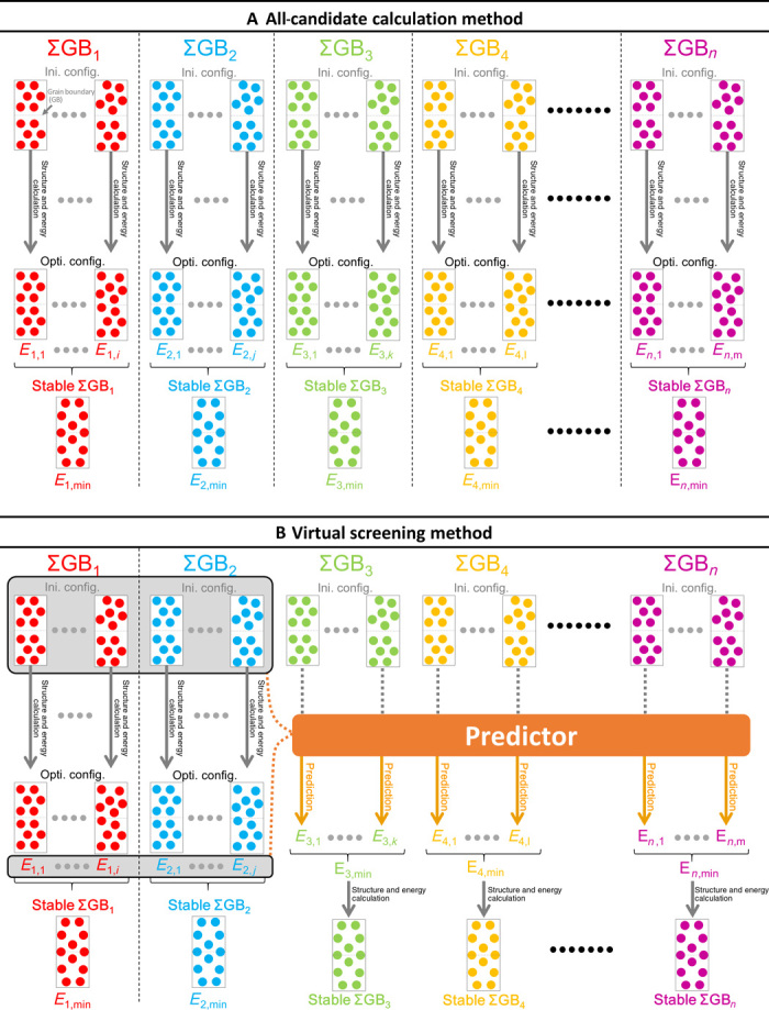
Schematic illustration of the method to determine the grain boundary (GB) structure and energy using the all-candidate calculation method (A) and the virtual screening method (B). Optimized configuration (Opti. config.) is obtained from the corresponding initial configuration (Ini. config.) via structure and energy calculations, using the first-principles method and the static lattice method.

To more efficiently determine the interface structure, a genetic algorithm method and a random structure–searching algorithm method have been proposed (19–24). In the genetic algorithm method, atomic structures of grain boundaries with lower grain boundary energy are generated with operations of selection, crossover, and mutation, and the stable grain boundary structures can be determined after a large number of generations. In the random structure–searching algorithm method, several hundred random structures are generated by randomly arranging atoms and ranked according to their energies after geometrical optimization. Although these approaches can efficiently determine unknown interface structures, more than several hundred trial calculations are still necessary to determine a single grain boundary structure. If the structure and energy of an unknown interface could be determined more efficiently, the investigation of interfaces would be markedly accelerated. This acceleration would lead to a deeper understanding of the mechanisms that give rise to interface properties.

Here, a virtual screening technique, which is an effective method in time-critical problems (25), was applied to determine the structure and energy of an interface. This virtual screening technique has been used in drug discovery, in which a prediction model is constructed using machine learning from a relatively small data set and a large database consisting of the actual data, and the data predicted by the prediction model are constructed. Then, the most promising candidate drug that will likely have the intended effectiveness is selected from the constructed large database. We applied this virtual screening technique to predict the structure and energy of interfaces. We demonstrate here that our virtual screening technique is very powerful and thus can determine the interface structure and energy.

RESULTS AND DISCUSSION

As a model grain boundary, we selected a series of [001] axis symmetric tilt CSL grain boundaries of face-centered cubic copper in this study, because numerous experimental and computational studies have been reported for this system. The CSL grain boundary of a single-element material has three degrees of freedom, namely, the rigid body translation of one side of the crystal with respect to the other side of the crystal in three dimensions.

Our virtual screening method is illustrated in Fig. 1B. A prediction model, namely, predictor, is constructed via regression analysis of the training data, in this case, ΣGB₁ and ΣGB₂. Once the predictor is constructed, the grain boundary energies can be predicted from the initial configurations. Then, the candidate configuration that will likely give the minimal energy, E_i,min (i = 3, 4, … n), can be determined. Next, the promising initial configuration is optimized using the structure and energy calculations. Finally, the accurate energy and stable structure are obtained (stable ΣGB_3–n in Fig.1B).

Here, 17 [001] axis symmetric tilt CSL grain boundaries of copper were considered: Σ5[001]/(210), Σ5[001]/(310), Σ13[001]/(230), Σ17[001]/(410), Σ17[001]/(350), Σ25[001]/(430), Σ25[001]/(710), Σ29[001]/(520), Σ29[001]/(730), Σ37[001]/(610), Σ37[001]/(750), Σ41[001]/(910), Σ41[001]/(540), Σ53[001]/(720), Σ53[001]/(950), Σ61[001]/(11 1 0), and Σ125[001]/(11 2 0). Each misorientation angle is listed in Fig. 2. Approximately 1,000,000 configurations must be considered to obtain stable structures for these grain boundaries. Namely, calculations must be performed 1,000,000 times to determine the structures of these grain boundaries. To construct the predictor, we selected Σ5[001]/(210), Σ5[001]/(310), Σ17[001]/(350), and Σ17[001]/(410) as the training data, corresponding to ΣGB₁ and ΣGB₂ in Fig. 1B. Those grain boundaries were selected as the training data from the viewpoint of the variance of their tilt angles and the computational costs for their calculations. Structure and energy calculations for a total of 150,000 configurations, corresponding to approximately 15% of all possible configurations, were performed. The most stable structures for Σ5[001]/(210), Σ5[001]/(310), Σ17[001]/(350), and Σ17[001]/(410) are shown in Fig. 3. Although only the structure from the projection view was previously reported, we can confirm that the calculated structures are almost identical to the previously reported structures (16, 26), indicating that these training data are suitable for constructing the predictor.

Fig. 2. Schematic illustration of symmetric tilt CSL grain boundary and the Σ values and misorientation angles (θ) of grain boundaries.

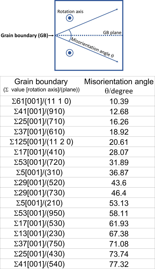
Fig. 3. The most stable structures in the training data.

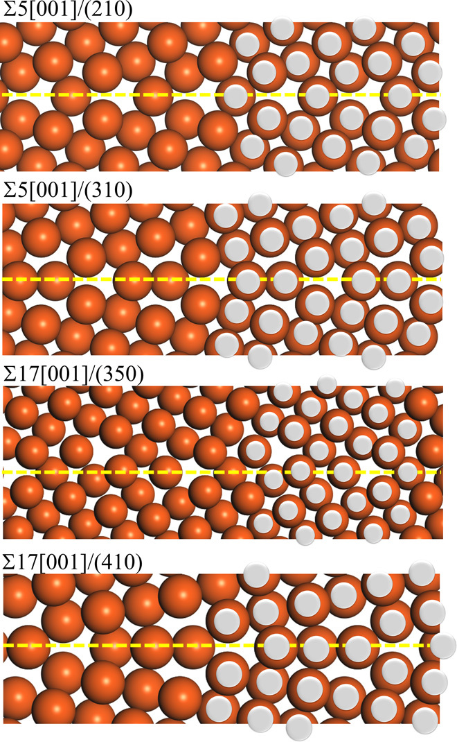
The most stable structures in the training data obtained by the all-candidate calculations: (from top to bottom) Σ5[001]/(210), Σ5[001]/(310), Σ17[001]/(350), and Σ17[001]/(410). Previously reported structures are overlaid with silver circles (16, 26).

To predict the grain boundary energies of noncalculated structures, the selection of descriptors for regression analysis is important. Here, geometrical data for the “initial atomic configurations” are used as the descriptors. This choice enables one to predict the grain boundary energy without performing the structure and energy calculations. The selected descriptors, such as the minimum bond length, maximum bond length, and so on, are listed in fig. S2. For the regression analysis, the nonlinear support vector machine (SVM) method was used, as described in Materials and Methods. As shown in section S3, SVM is a more suitable regression method in the present case as compared with the linear regression method.

The results of the regression analysis for the training data are shown in Fig. 4A. Most data lie on the gray line, indicating that the predicted energies are equal to the accurate energies and that the regression analysis succeeded in correctly constructing the predictor. To evaluate the accuracy of the constructed predictor, the predictor was applied to Σ13[001]/(230) as a test data. The results predicted by the predictor are shown in Fig. 4B. It is clear that most of the predicted grain boundary energies lie on the gray line, indicating that the constructed predictor is also suitable for the test data. This result implies that the constructed predictor has the potential to predict the energies of the grain boundaries before the structure and energy calculations.

Fig. 4. Result of regression analysis and calculated stable structures.

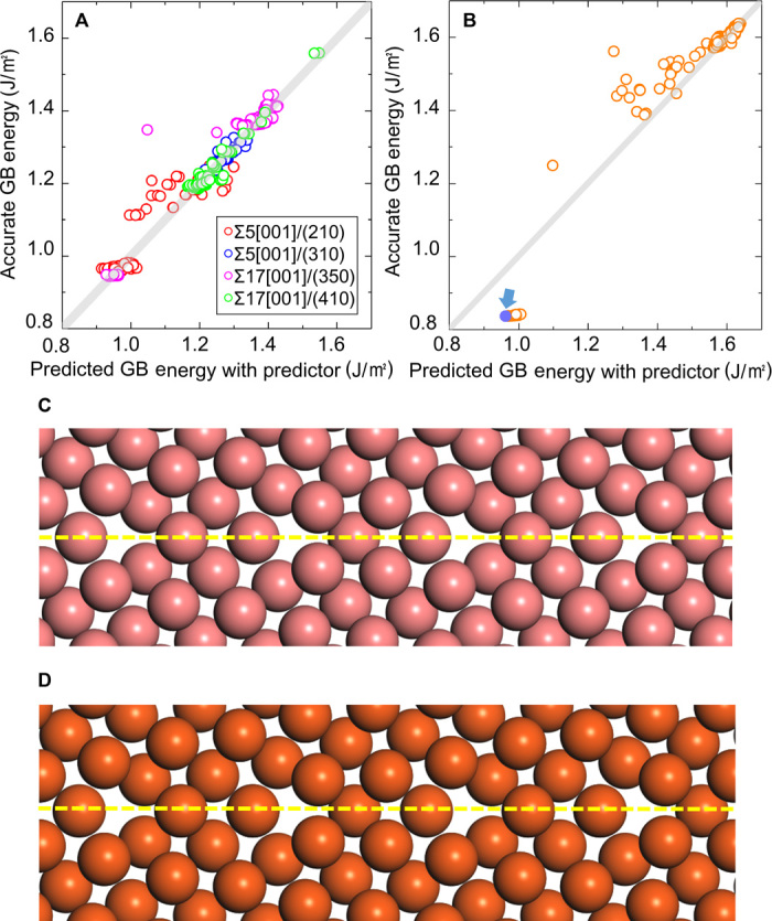
Predicted grain boundary energies and accurate grain boundary energies for the training data (A) and the test data (B). (C) The most stable structure of Σ13[001]/(230) obtained by the all-candidate calculations and (D) the structure predicted by the virtual screening method. Yellow lines represent the position of the grain boundary.

Here, we focus on the purple data point marked by the arrow in Fig. 4B. On the basis of the constructed predictor, the purple data point was predicted to provide the minimum grain boundary energy. The virtual screening method and the calculations of all candidates give the minimum grain boundary energy at the same purple data point. The predicted grain boundary energy is 0.96 J/m², which is only 10% larger than the minimum grain boundary energy obtained by the all-candidate calculations. It is also noteworthy that the predicted rigid body translation state (X = 5.0 Å, Y = 1.0 Å, and Z = 0.0 Å) is identical to the most stable rigid body translation state determined by the all-candidate calculations. Namely, we succeeded in screening all possible candidates and selecting the most promising candidate configuration to accurately provide the most stable structure. By performing the structure and energy calculation once for this rigid body translation state, we can obtain a grain boundary energy and structure identical to those obtained by the all-candidate calculations. Namely, the stable grain boundary structure and energy can be determined with only a one-time calculation using the present virtual screening method, which is significantly more efficient than the previously reported methods.

Here, on the basis of the constructed predictor, we predict the structures and energies of 12 other [001] axis symmetric tilt CSL grain boundaries: Σ25[001]/(430), Σ25[001]/(710), Σ29[001]/(520), Σ29[001]/(730), Σ37[001]/(610), Σ37[001]/(750), Σ41[001]/(910), Σ41[001]/(540), Σ53[001]/(720), Σ53[001]/(950), Σ61[001]/(11 1 0), and Σ125[001]/(11 2 0). As demonstrated for the test data (Fig. 4B) and schematically illustrated in Fig. 1B, the candidate configuration that provides the most stable structure was determined using the predictor, and the accurate grain boundary structure and energy were obtained by the one-time structure and energy calculations of this candidate configuration. Figure 5A shows the results of the predicted grain boundary energies and a comparison with previously reported grain boundary energies (17, 27). On the basis of previous studies, the grain boundary energy exhibits a convex profile in relation to the misorientation angle θ. The energy gradually increases with an increasing misorientation angle, reaching ~1.0 J/m² at 45°, and the energy then decreases at much higher misorientation angles. A detailed inspection reveals small cusps, namely, energy drops, at 16.26°, 28.07°, 36.87°, 53.13°, and 67.38°, corresponding to Σ25[001]/(710), Σ17[001]/(410), Σ5[001]/(310), Σ5[001]/(210), and Σ13[001]/(230), respectively.

Fig. 5. Predicted 13 grain boundary energies and a stable structure of Σ37[001]/(750).

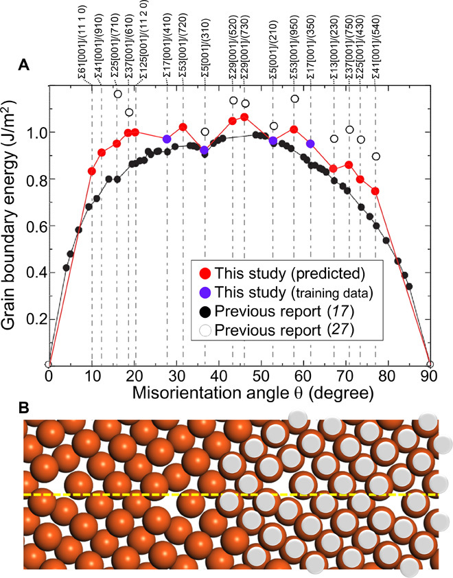
(A) Grain boundary energies as a function of the misorientation angle. Red and purple circles are obtained by the present method and all-candidate calculations, respectively, and open and filled black circles are obtained from previous studies. (B) Predicted stable structures for Σ37[001]/(750) in this study (orange circles) and in a previous report (silver circles) (26).

The predicted grain boundary energies of all grain boundaries obtained using the predictor are shown in Fig. 5A. Although the absolute value is not identical to that in previous studies owing to the difference in the empirical potential used, the overall profile of the grain boundary energy, displaying a convex shape with a maximum at 45°, is in agreement with previous reports (17, 27). Notably, small cusps at 16.26° and 67.38° are also reproduced by the prediction model (other cusps at 28.07°, 36.87°, and 53.13° were used for training). All atomic structures of the predicted grain boundaries are shown in fig. S4, and the results for Σ37[001]/(750) are compared with those of a previous report (26) in Fig. 5B. It is important to note that Σ37[001]/(750) is a type of low-symmetry grain boundary, and one must perform structure and energy calculations for the 69,053 possible configurations of 596 atom supercells in the all-candidate calculations. However, by using the present virtual screening method, the most stable structure fit to the previous report (26) can be obtained via a single calculation.

The abovementioned results demonstrate that the presented virtual screening method based on machine learning is sufficiently robust and powerful for predicting the stable interface structure and energy from initial atomic configurations. The success of this method implies that the initial atomic configuration is correlated to the grain boundary energy, and its correlation is studied by machine learning. It was already confirmed that the present method is applicable to other grain boundaries of metallic materials. To apply this method to ionic materials, such as oxides, it is expected that other descriptors on Coulomb interactions should be added. However, we would like to emphasize that the presented virtual screening method is not an “element-dependent” method and, thus, is generally applicable to the interfaces of any material system by selecting the suitable descriptors.

Finally, we consider the efficiency of the presented virtual screening method in finding the most stable grain boundary structure. The virtual screening method requires only one calculation for each boundary, whereas the all-candidate calculation method requires 850,000 calculations in total to determine the most stable structure among all of the abovementioned boundaries. The presented method significantly decreases the number of calculations to 13 because the candidate rigid body translation state is determined by the virtual screening method, and only a single calculation is necessary for each type of grain boundary. Namely, our method can achieve an efficiency that is 65,400 times higher than the brute force method. Moreover, the efficiency is much higher if the intended grain boundary has a higher Σ value. This high efficiency is greatly beneficial when the individual computational cost increases, such as for the use of a first-principles calculation or for a more complex grain boundary. In any case, our virtual screening method markedly enhances the speed in determining an interface structure.

CONCLUSIONS

In summary, we attempted to predict the structures and energies of grain boundaries using a virtual screening method based on machine learning. Geometrical factors of the initial configuration, such as the shortest bond length and local atomic density, were selected as the descriptors, and regression analysis was performed for the grain boundary energy using the nonlinear supporting vector machine. The prediction model, namely, predictor, was constructed using the grain boundary energy and structure information for four types of grain boundaries. The constructed predictor was then applied to 13 other grain boundaries. The present virtual screening technique successfully predicted energies and structures for these 13 grain boundaries. We demonstrated here that the virtual screening technique can achieve an efficiency that is more than several hundred to several tens of thousand times higher than the previously reported strategies.

Most notably, the descriptors acquired “before” the calculation were successfully used to describe the grain boundary energy, which is obtained “after” the calculation. Our study demonstrates that the initial configuration is correlated with the grain boundary energy. Furthermore, the correlations between the “before” and “after” calculations can be studied by machine learning and incorporated into the predictor. This finding implies that the present method has the potential to predict much more complex grain boundaries, such as those with much higher Σ values, random grain boundaries, or even heterointerfaces. We believe that our method will enhance our comprehensive understanding of interface phenomena in any material system.

MATERIALS AND METHODS

Computational methodology

With the all-candidate calculations, determining stable structures requires the calculation of various configurations in which one grain has been translated into three directions relative to the basis position, such as by using mirror symmetry, under periodic boundary conditions. Here, the same method was used to construct a data space for regression analysis. Lattice static calculations were performed with the conjugated gradient method using the GULP code (28). Let us consider the x and z axes as vectors on the grain boundary plane, with the z axis corresponding to the [001] tilt axis, and the y axis as a normal vector to the grain boundary plane. Rigid body translations into the x and z directions were conducted with a translational step size of 0.1 Å. Translations into the y direction had step sizes ranging from 1.0 to 1.5 Å in increments of 0.1 Å. Consequently, the number of initial configurations n was calculated as

$$\mathit{n}=\frac{{\mathit{L}}_{\mathit{x}}}{0.1}\times \frac{{\mathit{L}}_{\mathit{z}}}{0.1}\times 6$$

where L_x and L_z are lattice parameters of the supercells in the x and z directions, respectively. The number of configurations to the y direction corresponds to 6 (1.0 to 1.5). To prevent the grain boundary structures from transforming into the bulk structure, atoms located farthest from the grain boundaries were fixed, and the volume of cells was also fixed. The embedded-atom method potentials were used as empirical potentials (29). The grain boundary energies were estimated by the following formula

$${\mathit{E}}_{\text{GB}}=\frac{{\mathit{E}}_{\text{tot}}-{\mathit{E}}_{\text{bulk}}}{2\mathit{A}}$$

where E_tot is the total energy of the supercell with grain boundaries, E_bulk is the total energy of the supercell without grain boundaries, and A is the grain boundary area.

Here, the following 17 [001] axis symmetric tilt CSL grain boundaries of face-centered cubic Cu were investigated: Σ5[001]/(210), Σ5[001]/(310), Σ13[001]/(230), Σ17[001]/(410), Σ17[001]/(350), Σ25[001]/(430), Σ25[001]/(710), Σ29[001]/(520), Σ29[001]/(730), Σ37[001]/(610), Σ37[001]/(750), Σ41[001]/(910), Σ41[001]/(540), Σ53[001]/(720), Σ53[001]/(950), Σ61[001]/(11 1 0), and Σ125[001]/(11 2 0). Each grain boundary contains 44 to 1004 atoms. By considering the geometrical freedom of the three-dimensional rigid body translations, approximately 1,000,000 configurations must be considered.

Support vector regression analysis

Support vector regression (SVR) is a nonlinear regression analysis based on a SVM (30), which is a discriminant function using a kernel function. The loss function for ordinary regression analysis are sums of the squares of error, whereas that of SVR is an ε-insentisive error function and it benefits robust and sparse description. Furthermore, the kernel trick, which introduces kernel functions, enables fewer computations.

First, consider a data set {(x₁,y₁), …, (x_n,y_n)}, where x_i is a vector of descriptors and y_i is a response variable. In ε-SVR, the response and loss function are respectively described by

$$\mathit{f}(\mathit{x})={\mathit{w}}^{\mathrm{T}}\mathrm{\varphi }(\mathit{x})+\mathit{b}$$

and

$$\mathit{C}{\displaystyle \sum _{\mathit{i}=1}^{\mathit{n}}}{\mathit{E}}_{\mathrm{\epsilon }}({\mathit{y}}_{\mathit{i}},\mathit{f}({\mathit{x}}_{\mathit{i}}))+\frac{1}{2}{\Vert \mathit{w}\Vert }^2$$

where w is the weight vector, b is a bias parameter, C is the regularization parameter, φ(x) is the function that maps x to feature space, and f(x) is the response function. In the loss function, the first term is the sum of errors between predicted values and accurate ones, and the second term is a regularization term to prevent overfitting.

E_ε (y_n, f(x)) is denoted as

$${\mathit{E}}_{\mathrm{\epsilon }}({\mathit{y}}_{\mathit{i}},\mathit{f}({\mathit{x}}_{\mathit{i}}))=\{\begin{array}{cc}0& |{\mathit{y}}_{\mathit{i}}-\mathit{f}({\mathit{x}}_{\mathit{i}})|<0\\ |{\mathit{y}}_{\mathit{i}}-\mathit{f}({\mathit{x}}_{\mathit{i}})|-\mathrm{\epsilon }& |{\mathit{y}}_{\mathit{i}}-\mathit{f}({\mathit{x}}_{\mathit{i}})|\ge 0\end{array}$$

Then, by introducing nonnegative slack variables ξ_i and ξ^*_i, the above optimization problem is reduced to the following problem

$$\begin{array}{c}\underset{\mathit{w},\mathrm{\xi },\mathrm{\xi }*}{\text{min}}\mathit{C}{\displaystyle \sum _{\mathit{i}=1}^{\mathit{n}}}{\mathit{E}}_{\mathrm{\epsilon }}({\mathrm{\xi }}_{\mathit{i}}+{\mathrm{\xi }}_{\mathit{i}}^{*})+\frac{1}{2}{\Vert \mathit{w}\Vert }^2\\ \text{subject to} \{\begin{array}{c}\mathit{f}({\mathit{x}}_{\mathit{i}})\le {\mathit{y}}_{\mathit{i}}+\mathrm{\epsilon }+{\mathrm{\xi }}_{\mathit{i}}\\ \mathit{f}({\mathit{x}}_{\mathit{i}})\ge {\mathit{y}}_{\mathit{i}}-\mathrm{\epsilon }-{\mathrm{\xi }}_{\mathit{i}}^{*}\\ {\mathrm{\xi }}_{\mathit{i}},{\mathrm{\xi }}_{\mathit{i}}^{*}\ge 0\end{array}\end{array}$$

This optimization problem can be solved analytically as a dual problem by introducing the Lagrange function, similar to the following problem

$$\begin{array}{c}\underset{\mathrm{\alpha },\mathrm{\alpha }*}{\text{min}}\frac{1}{2}{(\mathrm{\alpha }-{\mathrm{\alpha }}^{*})}^{\mathrm{T}}\mathit{K}(\mathrm{\alpha }-{\mathrm{\alpha }}^{*})+\mathrm{\epsilon }{\displaystyle \sum _{\mathit{i}=1}^{\mathit{n}}}({\mathrm{\alpha }}_{\mathit{i}}+{\mathrm{\alpha }}_{\mathit{i}}^{*})+{\displaystyle \sum _{\mathit{i}=1}^{\mathit{n}}}{\mathit{y}}_{\mathit{i}}({\mathrm{\alpha }}_{\mathit{i}}-{\mathrm{\alpha }}_{\mathit{i}}^{*})\\ \text{subject to} \{\begin{array}{c}{\displaystyle \sum _{\mathit{i}=1}^{\mathit{n}}}({\mathrm{\alpha }}_{\mathit{i}}-{\mathrm{\alpha }}_{\mathit{i}}^{*})=0\\ 0\le {\mathrm{\alpha }}_{\mathit{i}},{\mathrm{\alpha }}_{\mathit{i}}^{*}\le \mathit{C}\end{array}\end{array}$$

where α and α^* are the Lagrange multipliers and K is a kernel matrix that consists of the kernel function k(x_i, x).

As a result, the response function or, in other words, the prediction model is written as

$$\mathit{f}(\mathit{x})={\displaystyle \sum _{\mathit{i}}^{\mathit{n}}}(-{\mathrm{\alpha }}_{\mathit{i}}+{\mathrm{\alpha }}_{\mathit{i}}^{*})\mathit{k}({\mathit{x}}_{\mathit{i}},\mathit{x})+\mathit{b}$$

in which α_i is a Lagrange coefficient and k means kernel function (now Gaussian-type function). This kernel function is made by the group of descriptor-vectors. Lagrange coefficients are 0 if the descriptor-vectors are not categorized to be the support vectors.

Here, the most stable structures and metastable structures of Σ5[001]/(210), Σ5[001]/(310), Σ17[001]/(410), and Σ17[001]/(350) were considered for the construction of the prediction model. We selected those grain boundaries as the training data from the viewpoint of the variance of tilt angles and the computational costs for their calculations. The result obtained when only Σ5[001]/(210) and Σ17[001]/(350) were used as the training data is shown in section S5. Because this selection is not suitable, the constructed model cannot be applied to the test data (fig. S5B).

The best parameters were selected from the following combinations: the margins of tolerance were 0.001, 0.01, 0.05, and 0.1; the penalty factors were 10, 100, 1000, and 10,000; and the variance values were 10⁻², 10⁻³, 10⁻⁴, and 10⁻⁵, namely, a total of 64 patterns. As a result, a margin of tolerance of 0.01, a penalty factor of 1000, and a variance of 10⁻⁴ were used for SVR parameters. Section S2 shows the descriptors used in performing the SVR. In addition to these descriptors, their square, inverse, exponential, and exponential inverse were considered. As a result, 83 descriptors were obtained, which were standardized to align their average and variance to 0 and 1, respectively. Section S6 shows the training and test data for the following parameters: margin of tolerance, 0.001; penalty factor, 100; and variance, 10⁻². As shown in section S6, the regression gives better results than that shown in Fig. 4A. However, the constructed predictor using these parameters does not work for the test data (fig. S6B).

This regression analysis focused on the relationships between the grain boundary energy and the initial atomic configuration before the structure and energy calculations. To perform this regression analysis more accurately, a smaller atomic relaxation during the calculation is preferable. From the calculated data, 800 results were screened for the SVR analysis.

SUPPLEMENTARY MATERIALS

Supplementary material for this article is available at http://advances.sciencemag.org/cgi/content/full/2/11/e1600746/DC1

section S1. The most straightforward method to determine the structure and energy of single grain boundary.

section S2. Descriptors used for the regression analysis in this study.

section S3. The results obtained through the linear regression method.

section S4. Predictions for 12 grain boundary structures using the virtual screening method.

section S5. Effect of the training data selection.

section S6. Effect of the parameters for the regression analysis.

fig. S1. Plot of the calculated grain boundary energies by the all-candidate calculation method.

fig. S2. Descriptors for the SVR analysis.

fig. S3. Predicted grain boundary energies through linear regression method.

fig. S4. Predictions for 12 grain boundary structures using the virtual screening method.

fig. S5. Predicted grain boundary energies with two of four kinds of grain boundary as the training data.

fig. S6. Predicted grain boundary energies under over-fitting.

REFERENCES AND NOTES

- 1.Ma C., Chen K., Liang C., Nan C.-W., Ishikawa R., More K., Chi M., Atomic-scale origin of the large grain-boundary resistance in perovskite Li-ion-conducting solid electrolytes. Energy Environ. Sci. 7, 1638–1642 (2014). [Google Scholar]
- 2.Lin Y., Fang S., Su D., Brinkman K. S., Chen F., Enhancing grain boundary ionic conductivity in mixed ionic-electronic conductors. Nat. Commun. 6, 6824 (2015). [DOI] [PMC free article] [PubMed] [Google Scholar]
- 3.Sato Y., Mizoguchi T., Oba F., Yodogawa M., Yamamoto T., Ikuhara Y., Atomic and electronic structure of [0001]/() Σ7 symmetric tilt grain boundary in ZnO bicrystal with linear current-voltage characteristic. J. Mater. Sci. 40, 3059–3066 (2005). [Google Scholar]
- 4.Sato Y., Yamamoto T., Ikuhara Y., Atomic structures and electrical properties of ZnO grain boundaries. J. Am. Ceram. Soc. 90, 337–357 (2007). [Google Scholar]
- 5.Yamaguchi H., Hiramatsu H., Hosono H., Mizoguchi T., The atomic structure, band gap, and electrostatic potential at the (112)[] twin grain boundary of CuInSe2. Appl. Phys. Lett. 104, 153904 (2014). [Google Scholar]
- 6.Möller J. J., Bitzek E., Fracture toughness and bond trapping of grain boundary cracks. Acta Mater. 73, 1–11 (2014). [Google Scholar]
- 7.Takigawa Y., Ikuhara Y., Sakuma T., Grain boundary bonding state and fracture energy in small amount of oxide-doped fine-grained Al2O3. J. Mater. Sci. 34, 1991–1997 (1999). [Google Scholar]
- 8.Nishimura H., Matsunaga K., Saito T., Yamamoto T., Ikuhara Y., Atomic structures and energies of Σ7 symmetrical tilt grain boundaries in alumina bicrystals. J. Am. Ceram. Soc. 86, 574–580 (2003). [Google Scholar]
- 9.Buban J. P., Mizoguchi T., Shibata N., Abe E., Yamamoto T., Ikuhara Y., Zr segregation and associated Al vacancies in alumina grain boundaries. J. Ceram. Soc. Jpn. 119, 840–844 (2011). [Google Scholar]
- 10.Lee H.-S., Mizoguchi T., Mistui J., Yamamoto T., Kang S.-J. L., Ikuhara Y., Defect energetics in SrTiO3 symmetric tilt grain boundaries. Phys. Rev. B 83, 104110 (2011). [Google Scholar]
- 11.A. P. Sutton, R. W. Balluffi, Interfaces in Crystalline Materials (Oxford Univ. Press, 1995). [Google Scholar]
- 12.Imaeda M., Mizoguchi T., Sato Y., Lee H.-S., Findlay S. D., Shibata N., Yamamoto T., Ikuhara Y., Atomic structure, electronic structure, and defect energetics in [001](310)Σ5 grain boundaries of SrTiO3 and BaTiO3. Phys. Rev. B 78, 245320 (2008). [Google Scholar]
- 13.Matsunaga K., Nishimura H., Saito T., Yamamoto T., Ikuhara Y., High-resolution transmission electron microscopy and computational analyses of atomic structures of [0001] symmetric tilt grain boundaries of Al2O3 with equivalent grain-boundary planes. Philos. Mag. 83, 4071–4082 (2003). [Google Scholar]
- 14.Milas I., Carter E. A., Effect of dopants on alumina grain boundary sliding: Implications for creep inhibition. J. Mater. Sci. 44, 1741–1749 (2009). [Google Scholar]
- 15.Milas I., Hinnemann B., Carter E. A., Structure of and ion segregation to an alumina grain boundary: Implications for growth and creep. J. Mater. Res. 23, 1494–1508 (2008). [Google Scholar]
- 16.Tschopp M. A., Mcdowell D. L., Asymmetric tilt grain boundary structure and energy in copper and aluminium. Philos. Mag. 87, 3871–3892 (2007). [Google Scholar]
- 17.Wolf D., Structure-energy correlation for grain boundaries in F.C.C. metals—III. Symmetrical tilt boundaries. Acta Metall. Mater. 38, 781–790 (1990). [Google Scholar]
- 18.Kohyama M., Yamamoto R., Doyama M., Structures and energies of symmetrical 〈011〉 tilt grain boundaries in silicon. Phys. Status Solidi B 137, 11–20 (1986). [Google Scholar]
- 19.Chua A. L.-S., Benedek N. A., Chen L., Finnis M. W., Sutton A. P., A genetic algorithm for predicting the structures of interfaces in multicomponent systems. Nat. Mater. 9, 418–422 (2010). [DOI] [PubMed] [Google Scholar]
- 20.Zhang J., Wang C., Ho K., Finding the low-energy structures of Si[001] symmetric tilted grain boundaries with a genetic algorithm. Phys. Rev. B 80, 174102 (2009). [Google Scholar]
- 21.Schusteritsch G., Pickard C. J., Predicting interface structures: From SrTiO3 to graphene. Phys. Rev. B 90, 035424 (2014). [Google Scholar]
- 22.Inoue K., Saito M., Wang Z., Kotani M., Ikuhara Y., On the periodicity of 〈001〉 symmetrical tilt grain boundaries. Mater. Trans. 56, 281–287 (2015). [Google Scholar]
- 23.Deaven D. M., Ho K. M., Molecular geometry optimization with a genetic algorithm. Phys. Rev. Lett. 75, 288–291 (1995). [DOI] [PubMed] [Google Scholar]
- 24.Zhao X., Shu Q., Nguyen M. C., Wang Y., Ji M., Xiang H., Ho K.-M., Gong X., Wang C.-Z., Interface structure prediction from first-principles. J. Phys. Chem. C 118, 9524–9530 (2014). [Google Scholar]
- 25.Pyzer-Knapp E. O., Suh C., Gómez-Bombarelli R., Aguilera-Iparraguirre J., Aspuru-Guzik A., What is high-throughput virtual screening? A perspective from organic materials discovery. Annu. Rev. Mater. Res. 45, 195–216 (2015). [Google Scholar]
- 26.Zhang L., Lu C., Michal G., Tieu A. K., Cheng K., Molecular dynamics study on the atomic mechanisms of coupling motion of [0 0 1] symmetric tilt grain boundaries in copper bicrystal. Mater. Res. Express 1, 015019 (2014). [Google Scholar]
- 27.Hasson G., Boos J.-Y., Herbeuval I., Biscondi M., Goux C., Theoretical and experimental determinations of grain boundary structures and energies: Correlation with various experimental results. Surf. Sci. 31, 115–137 (1972). [Google Scholar]
- 28.Gale J. D., GULP: A computer program for the symmetry-adapted simulation of solids. J. Chem. Soc. Faraday Trans. 93, 629–637 (1997). [Google Scholar]
- 29.Cleri F., Rosato V., Tight-binding potentials. Comput. Simul. Mater. Sci. 205, 233–253 (1991). [Google Scholar]
- 30.Vapnik V., Lerner A., Pattern recognition using generalized portrait method. Automation and Remote Control 24, 774–780 (1963). [Google Scholar]
Associated Data
This section collects any data citations, data availability statements, or supplementary materials included in this article.