The influence of large-scale wind power on global climate

Abstract

Large-scale use of wind power can alter local and global climate by extracting kinetic energy and altering turbulent transport in the atmospheric boundary layer. We report climate-model simulations that address the possible climatic impacts of wind power at regional to global scales by using two general circulation models and several parameterizations of the interaction of wind turbines with the boundary layer. We find that very large amounts of wind power can produce nonnegligible climatic change at continental scales. Although large-scale effects are observed, wind power has a negligible effect on global-mean surface temperature, and it would deliver enormous global benefits by reducing emissions of CO₂ and air pollutants. Our results may enable a comparison between the climate impacts due to wind power and the reduction in climatic impacts achieved by the substitution of wind for fossil fuels.

Global wind-power capacity is growing by ≈8GW·yr^-1, making wind the fastest growing nonfossil source of primary energy (1). The cost of electricity from wind power is now ≈40 dollars per MW·h^-1 at the best sites, and costs are declining swiftly (2). Wind power could play a substantial role in global energy supply when CO₂ emissions are strongly constrained to limit anthropogenic climatic change. Although the local environmental and aesthetic impacts of wind power have been explored, there has been little assessment of the climatic impacts of wind turbines.

Wind power is a renewable resource, but the rate of its renewal is finite and, in some respects, comparatively small. The yearly average horizontal flux of kinetic energy at the ≈100-m hub heights of large wind turbines can be >1kW·m^-2. These large power fluxes enable the economic extraction of wind power, but an array of wind turbines cannot extract this power arbitrarily because turbines interfere with their neighbors by slowing local winds. Most of the kinetic energy that drives wind turbines originates with the generation of available potential energy at planetary scales, which fuels winds throughout the atmosphere. Within the atmospheric boundary layer, turbulent mixing transports momentum downward to the surface and converts kinetic energy to heat by means of viscous (frictional) dissipation. The downward flux of kinetic energy averages ≈1.5 W·m^-2 over the global land surface (3). Ultimately, this small downward flux of kinetic energy limits the power that can be extracted by wind-turbine arrays (4).

Although the generation and dissipation of kinetic energy is a minor (≈0.3%) component of global energy fluxes, the winds mediate much larger energy fluxes by transporting heat and moisture. Therefore, alteration of kinetic energy fluxes can have much greater climatic effects than alteration of radiative fluxes by an equal magnitude (3, 5).

Methods

We explored the climatic impact of wind turbines by altering surface drag coefficients in a suite of numerical experiments using two different general circulation models, one of which was developed at the National Center for Atmospheric Research (NCAR) and the other of which was developed at the Geophysical Fluid Dynamics Laboratory (GFDL; Princeton). In each experiment, the drag coefficients were perturbed uniformly over an area defined by one of three wind-farm arrays, denoted A, B, and C (outlined in black in Figs. 1, 5A, and 5B, respectively). The reason for choosing these arrays is discussed below.

Fig. 1.

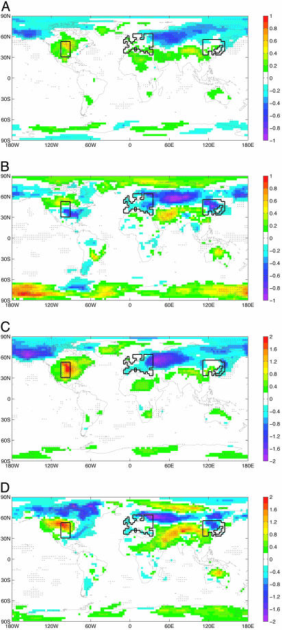
Wind-farm array and temperature response. Data are surface (2 m) air temperature, experiment minus control. Drag perturbation, δC_D, was 0.005 over the A wind-farm array outlined in black. Points that are significant at P > 0.9 by using a binary t test on annual/seasonal means are indicated (×). NCAR data are 37 yr of perturbed run composed of two runs with differing initial conditions and 108 yr of control composed of five independent runs. GFDL perturbed and control runs are both 20 yr long. NCAR (A) and GFDL (B) annual means are given, as well as NCAR (C) and GFDL (D) winter (December-February) means.

Fig. 5.

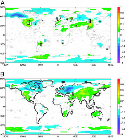
Surface-temperature response (δT_{2-m air}) to various configurations of wind-farm array and δC_D. (A) The B array covered 2.5% of global land surface. The roughness length z₀ was set to 5 m everywhere within the array, equivalent to δC_D ≅ 0.016 at the original 0.12-m areal-mean-roughness length of the array. Data are given for 50 yr of integration, δP = 15 TW. (B) Same as for A, but for the C array, with δC_D = 0.0006 globally (excepting Antarctica), 30 yr of integration, and δP = 30 TW.

We used two methods to parameterize the additional drag due to the turbines. The first method was a modification of the roughness length, z₀. In the boundary-layer parameterizations of the models (6, 7), z₀ determines the drag coefficient C_D, and ultimately, the surface fluxes through the following:

1

where z₁ is the height of the first-layer midpoint, k = 0.4 is the von Karman constant, and f is function that modifies C_D because of the influence of buoyancy on shear-driven turbulent mixing, which is parameterized by the Richardson number Ri. To simulate the effect of a uniform increase in drag, δC_D, we inverted the equation, treating f as constant, to solve for a z′₀ such that C_D(z′₀) - C_D(z₀) = δC_D. This approximation is reasonable because, on average, f departs only slightly from unity, and it departs the least when winds (and drag forces) are strongest.

Heat, momentum, and moisture have different surface-exchange coefficients, which are parameterized by using three different roughness lengths. In all of the results shown here, we made the same change in each coefficient. We tested the effect of changing z₀ for momentum only in a separate 20-yr run using the NCAR model. The results differed little from a run in which all roughness lengths were changed. However, because the B wind-farm array was used, the results cannot be compared quantitatively with the A results used throughout most of this article.

The second parameterization was an explicit drag scheme. Although the specifics differed, the result in both models was to add the following new component:

2

to the model physics in the lowest two layers, where C_ED is the explicit drag coefficient and Δz is the layer thickness. In the NCAR model, the drag was applied to the lowest two layers with midpoints at 65 and 250 m, with a C_ED/Δz quotient of 17 × 10^-5 and 0.8 × 10^-5 m^-1, respectively. In the GFDL model, the midpoints are at 37 and 180 m, with a C_ED/Δz of 0.8 × 10^-5 and 1.6 × 10^-5 m^-1. These values were chosen to represent an array of wind turbines, 2.8 turbines per km², each with 100-m-diameter rotors and 100-m hub heights that remove 40% of kinetic energy of the resolved flow.

Experiments at NCAR used the Community Atmospheric model cam (version 2.0.1), which was run at its standard resolution (26 hybrid vertical layers, with T42 dynamics mapped to a 2.8 × 2.8° horizontal grid) (7). Experiments at GFDL used the new am2 Atmospheric Model (version p10), which was run at its standard resolution [18 hybrid vertical layers with grid-point dynamics on a 2.0 × 2.5° (latitude × longitude) horizontal grid] (8).

For the NCAR model, the perturbed model runs were compared with 108 yr of control integration composed of five control runs of various lengths, each initiated with a random perturbation of the initial temperature field to assure independence. For the GFDL model, a single 20-yr control run was used. All model runs used climatological sea-surface temperatures.

The Relationship Between Large-Scale Drag and Wind-Farm Properties

Large increases in drag coefficient will certainly alter climate; the challenge is to relate the drag perturbation and resulting climate response to the amount of power generated by the wind turbines.

The increased drag coefficient, δC_D, removes energy from the resolved flow with an areal flux of ρv³δC_D. We call the global integral of this flux δP, the additional power dissipated by surface friction due to the additional drag. In both models, δP was computed by running the surface physics of the model twice at each time step once with original z₀ and once with the perturbed z′₀ to compute the change in surface stress and then computing at the lowest model layer, which is a direct measure of the additional kinetic energy dissipation at the surface.

Only a fraction of δP goes into electricity. A turbine removes resolved kinetic energy at a rate given by the force on the turbine times the free-stream velocity. Normalizing this quantity by the power flowing through a disk the size of the rotor at free-stream velocity yields the drag coefficient for the turbine, C_D. Normalizing the electricity produced by this same quantity yields the power coefficient, C_P. Therefore, the fraction of energy removed from the atmosphere (δP) that is converted into electricity is C_P/C_D. In practice, at typical velocities, C_P ranges (9, 10) from 0.35 to 0.4 and C_D ranges from 0.7 to 0.75, yielding an atmospheric efficiency of 47-57%. Including the effects of turbine-generated turbulence might significantly lower the effective atmospheric efficiency by increasing turbulent momentum transport and thus inducing additional drag on the ground downstream of the turbines. Additional turbulence will also increase turbulent transport of heat and moisture (11). Both effects are ignored here, and thus, we may underestimate the climate impacts per unit electricity.

Measurements at the San Gorgonio Pass wind farm in California show average δC_D = 0.007 at hub height (Neil Kelley, National Wind Technology Center, Golden, CO, personal communication). These measurements are for a wind farm with ≈20-m turbine hub heights, and they may underestimate the drag that would be produced by large wind farms built during the next decades in which mean hub heights are likely to be >100 m. A recent analytic model of the interaction of wind turbines arrays with the boundary-layer flow predicts a δC_D (at 80 m) of 0.013-0.005 for average turbine spacings of five to eight rotor diameters, assuming a 100-m turbine hub height (12).

We used drag perturbations of 0.0006-0.016 at the 80-m reference height of the model. Wind farm δC_D values greater than ≈0.003 are likely to be unrealistic when averaged over the scale of a general circulation models grid cell; we used larger δC_D values only to test the climate response of the model and to improve the signal/noise ratio. The smallest δC_D values used here were approximately one order of magnitude less than the value of δC_D that was expected from typical wind farms, equivalent to filling ≈1/10th of a grid cell with wind farms.

Results

Fig. 1 shows the response of near-surface temperature to an increase in z₀ adjusted to produce a nearly uniform increase of 0.005 in drag coefficient, δC_D, over the wind-farm array outlined in black. This array was chosen to (i) be simple; (ii) be near areas of high energy use; (iii) have good wind resources (mean of ½ ρv³); (iv) avoid high topography; (v) cover the northern extra-tropics only to simplify analysis of changes in general circulation; and (iv) have sufficient area to allow good signal/noise ratio over a range of δC_D. The array covers 10% of the global land surface. The increase in local kinetic energy dissipation (power) due to the added drag, δP, is 21 and 13 TW for the NCAR and GFDL models, respectively.

Although the change in global-mean surface air temperature is negligible, regional peak-seasonal responses exceed ±2°C. Note the similarities between the two models over most of the globe and that winter-season cooling over most of Europe contrasts with winter-season warming over temperate (NCAR) or central (GFDL) North America.

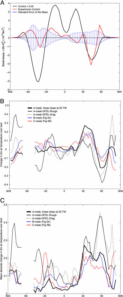
Within the northern extratropics note that (i) the magnitude of the response is approximately as large outside the areas with drag perturbation as it is within them, (ii) the sign of the response is not the same in each of the three areas, and (iii) the zonal pattern of response is similar across both models and all drag perturbations (see Fig. 6B). These facts suggest that the primary mechanisms are nonlocal (i.e., that the climatic effects are not dominated by local changes in the surface energy budget due to the presence of increased surface drag). We speculate that these effects arise, in part, from perturbation of poleward heat transport (13).

Fig. 6.

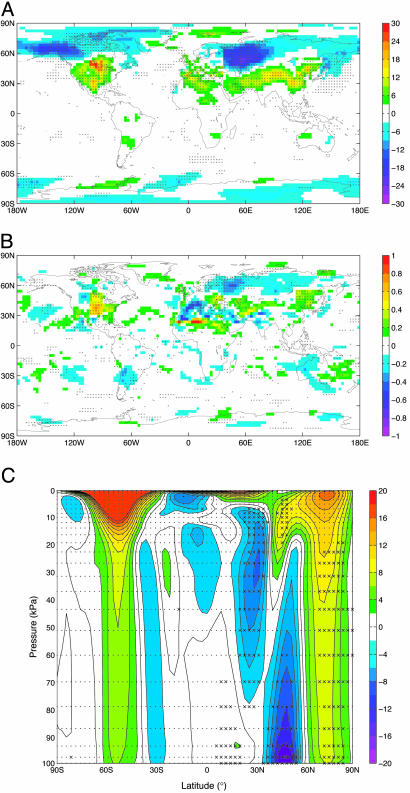
Zonal measurements of climatic response. (A) Torque. Data are given from the NCAR model as described in Fig. 1 A. [The plotted quantity is F(θ)cos²(θ), which is torque per radian of latitude divided by , where R_E is the earth's radius and F(θ) is the zonal stress.] Note how the torque added by the wind-farm drag at ≈30-60°N is redistributed so that total torque remains at zero. (B) Zonal and annual mean δT_{2-m air} over land. Black lines show response to the A array shown in Fig. 1. Red and blue lines show data from the experiments using different wind farm configurations shown in Fig. 5. All lines correspond to single-model runs except the thick black line, which is derived from the linear response data of Fig. 3A scaled with an arbitrary 25 TW δP. (C) Same as for B, but for zonal means of the absolute magnitudes.

Last, the climatic response is constrained by our use of prescribed climatological sea-surface temperatures. The magnitude of the wind-power-induced changes will be different, and possibly larger, when models are run with an interactive ocean in which this constraint is relaxed.

In Figs. 1 and 5, points at which the perturbation and control runs were different at the 90% level in a t test computed for annual or seasonal means are indicated (×). The t test is suspect here because it assumes a frequency-independent (white) noise-power spectrum, and thus, the indicated points should be interpreted with caution. Statistical significance is difficult to establish in experiments with atmospheric models because of spatiotemporal correlations (14). Here, we rely on the monotonicity of relationships between the size of the perturbation and the climactic response to demonstrate that the perturbations have nonrandom effects (Figs. 2, 3, 4).

Fig. 2.

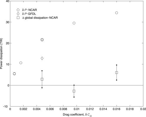
Energy dissipation versus drag. Statistical uncertainty in δP is negligible. The ensemble of seven NCAR “linearity” model runs are shown (there are two points at δC_D = 0.0006 and δC_D = 0.005). The change in global-mean surface dissipation (experiment control) is <1% of the control mean of 1.7 W·m^-2, or 850 TW.

Fig. 3.

Linear coefficient of climatic response in NCAR-linearity ensemble. In all plots, the magnitude at each point is the slope of a least-squares linear fit of the deviation in the given variable with respect to the global δP values using one datum from each of the seven linearity runs shown in Fig. 2. The y intercepts are constrained to zero. Points at which the correlation between the variable and δP was significant at P > 0.9 are indicated (×). (A) Annual mean δT_{2-m air} in mK·TW^-1. (B) Ratio change in annual mean precipitation in % TW^-1. (C) Annual mean change in zonal wind in mm·sec^-1·TW^-1. Note that the dipole corresponds to a shift toward the pole of the northern-hemisphere jet.

Fig. 4.

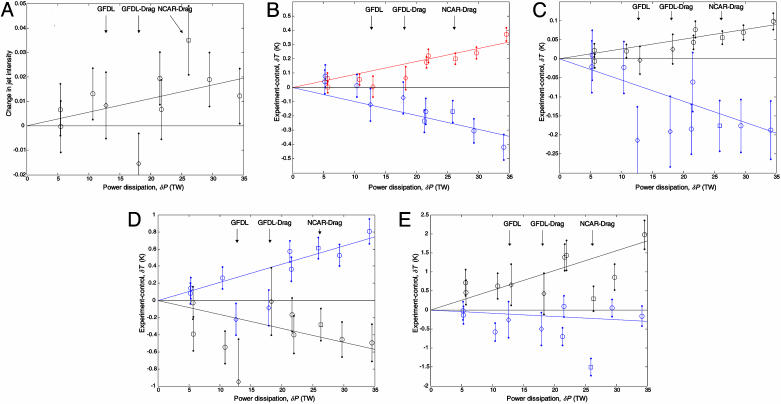
Mean climatic response over various masks versus δP. In each plot, the x axis is δP, corresponding to the y axis of Fig. 2. For each point, the seasonal means of a given model run are first integrated over a mask, and differences and standard errors are then computed by using the set of mask integrals for all model years in the experiment and control runs. Results from 10 model runs are shown, all of which use the A array shown in Fig. 1. ○, Data from the seven elements of the NCAR ensemble; □, NCAR drag physics run; and ⋄, data from the two GFDL runs in which the 13 and 18 TW points indicate the roughness length and drag physics runs, respectively. (A) Relative decrease in intensity of the northern-hemisphere jet over a mask that extends from 40-60°N and 100-30 kPa. (B) Annual mean δT_{2-m air} averaged over two separate masks. The red and blue points use a mask defined by the points that are positive and negative, respectively, as well as significant in Fig. 3A. (C) Annual mean δT_{2-m air} over zonal land-surface masks at 25-45°N (black) and 55-65°N (blue). (D) Summer (June-August) δT_{2-m air} for the North American (black) and European (blue) areas of the A wind-farm array shown in Fig. 1. (E) Same as for D, but for winter (December-February).

To provide a reference response with which to compare alternative models and parameterizations, and to explore how the magnitude of climatic response depends on the amount of extracted wind power, δC_D was varied in an ensemble of seven (≈20-yr-long) model integrations, each of which used the array shown in Fig. 1. The resulting δP values and the change in global surface dissipation are shown in Fig. 2.

We draw two interesting conclusions from these results. First, the effectiveness with which increasing δC_D extracts additional power declines with δC_D because surface winds decrease with increasing drag. Second, the increase in surface drag has a negligible effect on the global dissipation of kinetic energy at the surface. Surface winds outside the wind-farm array are slowed so that dissipation outside the array area decreases to compensate for the increased dissipation within the array. The reason that the compensation is so complete is likely that the generation of available kinetic energy, as well as its dissipation outside the boundary layer, depend on a large-scale atmospheric structure that varies only slightly in response to the changes in surface drag; also, near-surface sink must equal atmospheric source.

Assessments of wind-power capacity assume that regional or global capacity can be estimated by summing the local wind resource (15, 16). Our results suggest that large-scale atmospheric dynamics provide a rough upper bound on the power that can be extracted by wind farms over a specific region, just as wind-shadowing effects constrain the distribution of turbines in existing wind farms (17).

We estimated the climatic response to δP by regressing observed climatic change against δP over the ensemble (Fig. 3). In addition to providing a clean measurement of climatic response across the ensemble, this method provides a test of significance that is uncontaminated by assumptions about the temporal noise spectrum that are embedded in the significance test shown in Figs. 1 and 5.

We compared response across models and parameterizations by plotting various integrated measurements of response versus δP (Fig. 4). Responses are generally similar across models and parameterizations, with a couple of obvious exceptions (i.e., the difference between the two GFDL parameterizations in Fig. 4A). In particular, the climatic response to a change in δP with the roughness parameterization was not systematically either lower or higher than it was with the drag parameterization.

The roughness-length modification is perhaps the more robust of the two parameterizations because, in changing a model parameter, we left the self-consistency of the model physics unaltered. However, it is not yet clear how accurately wind turbines are represented by a change in surface roughness. The explicit drag formulation is perhaps more physically realistic, but the results must be treated with caution because we have not thoroughly explored the interaction of the new drag term with existing model physics. Moreover, the drag parameterization excludes important processes, such as the direct effects of wind turbines on turbulence. Results from a mesoscale model suggest that including the generation of turbulence by wind farms greatly increases their climatic influence (11).

Over the northern midlatitudes, the wind-farms increase mean C_D over land by ≈20% for δC_D = 0.005. The added drag slows midlatitude winds by a few percentage points (Fig. 4A), shifts the jet toward the pole (Fig. 3C), and increases surface stress by ≈5% (Fig. 6A). Collectively, these results demonstrate that increased drag in areas comprising only 10% of global land surface can produce statistically significant changes in the general circulation. Given that τ ∝ C_Dv², these changes are consistent with the assumption that winds slow sufficiently to approximately conserve surface dissipation in response to increasing drag.

The ensemble results allow a rough assessment of the functional form of the climatic response for δP up to 25 TW (see the points marked with ○ in Fig. 4). The 25-TW perturbation is an ≈4% alteration of global surface energy dissipation, or an ≈20% change in drag over northern-hemisphere land. Within the limits of the experimental error, the results suggest that the climatic response is often approximately linear for δP up to 25 TW (Fig. 4 A; C, black; and D, blue and black) but might be saturating (Fig. 4D, black) or sigmoid with a threshold (Fig. 4C, blue), at least in some cases.

A useful quantity for assessing the climatic impacts of wind power is the derivative of climatic response with respect to wind-power-induced dissipation (δP) for small amounts of dissipation (δP → 0). The point-by-point linear fits to δP described above (Fig. 3) provide a estimate of this derivative. Uncertainty in our estimate of the derivative at δP → 0 will arise from three sources, (i) nonlinearity in climate response, (ii) errors due to random climate variability in the individual model runs, and (iii) systematic error due to deficiencies in the model physics.

Climatic response will be increasingly linear (18, 19) as δP → 0 because, while we are interpreting changes in δC_D as a variation in wind power from zero, the climate model is in fact responding to small changes in drag from the prescribed background C_D. Therefore, the rough linearity observed at large δP suggests that nonlinearity introduces comparatively small errors in our estimate of the response as δP → 0. Errors due to random climate variability are similarly small. The dominant error in estimating the small-signal response almost certainly arise from deficiencies in the physics of the model and our parameterization of wind-turbine-induced drag. The differences between responses in the two models and the two parameterizations suggests that these model-related systematic errors may be of order unity.

The patterns of climatic response shown in Figs. 1, 2, 3, 4 result from the particular configuration (A) of wind-farm array shown in Fig. 1. The response to alternative B and C configurations are shown in Fig. 5. One might suppose that the effects depended strongly on the high density of turbines in the wind farms and that a uniform global distribution of δC_D that generated similar δP would produce a much smaller climatic response. We tested this hypothesis in the NCAR model by setting δC_D = 0.0006 over all land except Antarctica (the C configuration). The resulting δP was 30 TW, which is approximately five times larger than the 6-TW dissipation produced by using the same δC_D in the A configuration that covers 10% of the land surface (see the δC_D = 0.0006 points in Fig. 4). The surface-temperature response to distributed δC_D (Fig. 5B) was of approximately similar peak magnitude to that resulting from a δP of 21 TW generated in the A configuration (Fig. 1), suggesting that a uniform distribution of δC_D does not drastically reduce the magnitude of climate impacts for a given δP. Some similarities are evident across all three wind-farm configurations: in all experiments the surface-temperature response is of approximately similar peak magnitude, and there is surprising consistency in the zonal pattern of temperature response (Fig. 6 B and C).

Implications

The climatic impact of wind power is currently negligible in comparison with other anthropogenic climate forcings. Suppose that use of wind power were to grow 100-fold to 2 TW, which is somewhat beyond the largest quantity envisaged for the next half century by recent studies (20, 21) but only ≈1/10th of the global electricity demand in 2100 under fossil-intensive emissions scenarios (22). At an atmospheric efficiency of 50%, 2 TW of wind power corresponds to a δP of 4 TW, which is similar to the smallest δP used here. Our results suggest that the resulting peak changes in seasonal mean temperature might be ≈0.5 K, with RMS changes approximately one order of magnitude smaller and near-zero change in global mean temperature (using the method shown in Fig. 3A with winter means produces maximum values of ≈0.1KTW^-1, see also the δC_D = 0.0006 points of Fig. 4 D and E). These climatic changes are detectable above background climatic variability in model runs of a few decades in duration, but they might remain too small to detect in the presence of other anthropogenic change and natural climate variability.

A single wind turbine has an infinitesimal direct effect on global climate, but it also makes an infinitesimal indirect contribution to reducing climate change by slowing the growth of atmospheric CO₂. The ratio of direct to indirect effects is relevant to decisions about implementing wind power at any scale if the objective is to mitigate climate change.

The direct impact of wind power is immediate, whereas the indirect climatic benefit grows from zero with time as electricity from wind reduces CO₂ emissions and slows the growth of concentrations. A comparison of the effects depends, among other factors, on (i) how impacts at different times and locations are aggregated, (ii) the effectiveness of electricity from wind in reducing CO₂ emissions, and (iii) the baseline CO₂ emission profile.

As an illustrative example, we compare the time-averaged direct and indirect effects of generating 0.1 TW of wind power computed over 1 century with no discounting.** At an atmospheric efficiency of 50%, the peak magnitude of the direct temperature change will be ≈6 mK (Fig. 3A). Assuming that wind power displaces CO₂ emissions at the global electric-sector carbon emissions intensity, 0.1 TW of wind power will reduce annual emissions by ≈0.15 GtC (gigatons of carbon), which will reduce century-average CO₂ concentrations by ≈1.6 ppm. Assuming that climate sensitivity to small perturbations in CO₂ concentration is linear with a slope given by a linear extrapolation of the 550-ppm equilibrium response, wind power would reduce the response by ≈0.6%, reducing peak temperature changes by ≈30 mK. Under these assumptions, the peak direct effect is approximately one-fifth of the peak indirect effect. However, these assumptions were chosen for ease of exposition and each can be readily challenged.

The direct climatic changes that are due to wind power may be beneficial because they can act to reduce, rather than increase, aggregate climate impacts. For example, assume that impacts are proportional to the local squared-deviation of temperature from preindustrial means and that a small climate change due to wind power with the pattern of response shown in Fig. 3A is superimposed on a much larger CO₂-induced warming. In this case, the polar cooling and low-latitude warming from wind power tends to reduce aggregate impacts due to CO₂-induced warming, which has the opposite pole-to-equator gradient, even though the average temperature change due to wind power is zero.

A more systematic analysis would need to use the tools developed in integrated assessment models of climate change, and it would need to account for the spatial distribution of the climatic changes and the sensitivity to climate impacts. Preliminary calculations using assumptions common in such models consistently show that, by reducing CO₂ emissions, the indirect benefits of wind turbines exceed the costs (or benefits) arising from their direct climatic effects. However, additional work is necessary to determine whether these impacts are large enough to be included routinely in assessments because preliminary estimates of the ratio of direct to indirect effects range from a few percent to near unity, depending on assumptions.

Our analysis suggests that the climatic impacts of wind power may be nonnegligible, but they do not allow a detailed quantitative evaluation of the climatic changes induced by extraction of wind power. Further research is warranted on the local effects of current wind farms on surface climate and boundary-layer meteorology, as well as on the development of better parameterizations of wind farms in large-scale models. Last, it may be comparatively easy to reduce the climatic impacts of wind turbines. Preliminary analysis suggests that turbine designs could be modified to increase the atmospheric efficiency (C_P/C_D) by several tens of percent and reduce the generation of turbulence by several fold, both of which could be done economically. Additional mitigation of impact might be achieved by siting wind farms such that their effects partially cancel and by tailoring the interaction of turbines with the local topography to minimize the added drag.

References

- 1.American Wind Energy Association. (2004) Global Wind Energy Market Report (American Wind Energy Association, Washington, DC).
- 2.McGowan, J. G. & Connors, S. R. (2000) Annu. Rev. Energy Environ. 25, 147-197. [Google Scholar]
- 3.Peixoto, J. P. & Oort, A. H. (1992) Physics of Climate (American Institute of Physics, New York).
- 4.Best, R. W. B. (1979) Energy Conver. 19, 71-72. [Google Scholar]
- 5.Keith, D. W. (1996) in Encyclopedia of Climate and Weather, ed. Schneider, S. H. (Oxford Univ. Press, New York), pp. 278-283.
- 6.Holstlag, A. A. M. & Boville, B. A. (1993) J. Clim. 6, 1825-1842. [Google Scholar]
- 7.Collins, W. D., Hack, J. J., Boville, B. A., Rasch, P. J., Williamson, D. L., Kiehl, J. T., Briegleb, B., McCaa, J. R., Bitz, C., Lin, S.-J., et al. (2003) Description of the NCAR Community Atmospheric Model (CAM2) (National Center for Atmospheric Research, Boulder, CO).
- 8.The GFDL Global Atmospheric Model Development Team (2004) J. Clim., in press.
- 9.Gipe, P. (1995) Wind Energy Comes of Age (Wiley, New York).
- 10.Bossanyi, E. A., Maclean, C., Whittle, G. E., Dunn, P. D., Lipman, N. H. & Musgrove, P. J. (1980) in Proceedings of the Third International Symposium on Wind Energy Systems, (Lyngby, Denmark), pp. 401-416.
- 11.Baidya Roy, S., Pacala, S. W. & Walko, R. L. (2004) J. Geophys. Res. Atmos. 109, D19101. [Google Scholar]
- 12.Frandsen, S. & Thøgersen, M. L. (1999) Wind Eng. 23, 327-339. [Google Scholar]
- 13.Robinson, W. A. (1997) J. Clim. 10, 176-182. [Google Scholar]
- 14.Livezey, R. E. & Chen, W. Y. (1983) Monthly Weather Rev. 111, 46-59. [Google Scholar]
- 15.Intergovernmental Panel on Climate Change Working Group III (2001) in Climate Change 2001: Mitigation. Contribution of Working Group III to the Third Assessment Report of the IPCC, eds. Metz, B., Davidson, O., Swart, R. & Pan, J. (Cambridge Univ. Press, Cambridge, U.K.).
- 16.Grubb, M. J. & Meyer, N. I. (1993) in Renewable Energy: Sources for Fuels and Electricity, eds. Johansson, T. B. & Burnham, L. (Island, Washington, DC), pp. 157-212.
- 17.Frandsen, S. (1992) J. Wind Eng. Ind. Aerodyn. 39, 251-265. [Google Scholar]
- 18.Mitchell, T. D. (2003) Clim. Change 60, 217-242. [Google Scholar]
- 19.Sexton, D. M. H., Grubb, H., Shine, K. P. & Folland, C. K. (2003) J. Clim. 16, 1320-1336. [Google Scholar]
- 20.European Wind Energy Association (2003) Wind Force 12: A Blueprint to Archive 12% of the World's Electricity from Wind Power by 2020 (European Wind Energy Association, Brussels).
- 21.Edmonds, J., Clarke, J., Dooley, J., Kim, S. H. & Smith, S. J. (2004) Energy Econ., in press.
- 22.Nakiâcenoviâc, N. & Swart, R. eds. (2000) Special Report on Emissions Scenarios: A Special Report of Working Group III of the Intergovernmental Panel on Climate Change (Cambridge Univ. Press, Cambridge, U.K.).
- 23.Houghton, J., Filho, L. M., Bruce, J., Lee, H., Callander, B., Haites, E., Harris, N. & Maskell, K. eds. (1995) Climate Change, 1994: Radiative Forcing of Climate Change and an Evaluation of the IPCC IS92 Emission Scenarios (Cambridge Univ. Press, Cambridge, UK).
- 24.Enting, I. G., Wigley, T. M. L. & Heimann, M. (1994) Future Emissions and Concentrations of Carbon Dioxide: Key Ocean/Atmosphere/Land Analyses (Commonwealth Scientific and Industrial Research Organisation, Division of Atmospheric Research, Canberra, Australia).