A new universal dynamic model to describe eating rate and cumulative intake curves^,,

Abstract

Background: Attempts to model cumulative intake curves with quadratic functions have not simultaneously taken gustatory stimulation, satiation, and maximal food intake into account.

Objective: Our aim was to develop a dynamic model for cumulative intake curves that captures gustatory stimulation, satiation, and maximal food intake.

Design: We developed a first-principles model describing cumulative intake that universally describes gustatory stimulation, satiation, and maximal food intake using 3 key parameters: 1) the initial eating rate, 2) the effective duration of eating, and 3) the maximal food intake. These model parameters were estimated in a study (n = 49) where eating rates were deliberately changed. Baseline data was used to determine the quality of model's fit to data compared with the quadratic model. The 3 parameters were also calculated in a second study consisting of restrained and unrestrained eaters. Finally, we calculated when the gustatory stimulation phase is short or absent.

Results: The mean sum squared error for the first-principles model was 337.1 ± 240.4 compared with 581.6 ± 563.5 for the quadratic model, or a 43% improvement in fit. Individual comparison demonstrated lower errors for 94% of the subjects. Both sex (P = 0.002) and eating duration (P = 0.002) were associated with the initial eating rate (adjusted R² = 0.23). Sex was also associated (P = 0.03 and P = 0.012) with the effective eating duration and maximum food intake (adjusted R² = 0.06 and 0.11). In participants directed to eat as much as they could compared with as much as they felt comfortable with, the maximal intake parameter was approximately double the amount. The model found that certain parameter regions resulted in both stimulation and satiation phases, whereas others only produced a satiation phase.

Conclusions: The first-principles model better quantifies interindividual differences in food intake, shows how aspects of food intake differ across subpopulations, and can be applied to determine how eating behavior factors influence total food intake.

INTRODUCTION

In 1980, Kissileff et al. (1) developed and used the Universal Eating Monitor to rigorously quantify differences in human eating rates during the ingestion of liquids or solid food. Universal Eating Monitors capture data on food intake over time by tracking the grams of food that have been removed and consumed by a participant whose plate is on a scale. Graphically, the data are plotted as a cumulative intake curve, where time (in minutes) is plotted on the horizontal axis and the food consumed (in grams) appears on the y axis. By evaluating differences in the curve’s shape and form, investigators can objectively compare eating rates and total food consumed (2). Indeed, the Universal Eating Monitor has been critical for understanding behaviors involving eating disorders (3, 4) and obesity (5–7), in which eating patterns deviate from the norm.

To model human eating behavior, Kissileff et al. (1) used lines and quadratic functions fit to cumulative food intake data. In both models, the linear coefficients represent the initial eating rate (the initial rate of food intake), whereas in the quadratic model twice the quadratic coefficient can be thought of as the “eating acceleration” or the rate of change of the eating rate (8, 9). These linear and quadratic models were used for their simplicity, ease of comparison (10), and capacity to compare coefficients between different populations (1, 3, 11).

Although linear and quadratic models are expedient approximations when the gustatory stimulation is weak, they unfortunately suffer from certain drawbacks that limit their application. For instance, in the case of linear models, they assume that the eating rate is constant, so they cannot be used to model gustatory stimulation (speeding up of the eating rate) or satiation (slowing down of the eating rate) and do not model the plateau value that the individual’s food intake approaches as the “maximal food intake,” or the individual’s limit on the amount of food they can consume (under the specific conditions). Quadratic models of the form ct² + bt + a have therefore been championed instead. In this case, the feedback response of satiation if c < 0 or, alternatively, gustatory stimulation if c > 0 can be approximated (10). Although clearly an improvement over the linear models, the quadratic model also has shortcomings. First, because the sign of c is constant, quadratic functions cannot simultaneously model both stimulation (eating rate speeding up) and satiation (eating rate slowing down). Second, because quadratic functions model cumulative intake data as increasing and then eventually declining (Figure 1A), they are also incapable of modeling the “food plateau.” This represents a limitation because the model cannot accurately predict what happens for a longer eating duration. Third, to derive an optimal quadratic model curve fit, a nonzero constant term, a, must be added to the model (10). The constant term, colloquially referred to as a “fudge factor,” is an artifact of improper curve fitting (8) defined as an ad hoc quantity introduced into a model to make it fit observations or expectations. This constant fudge factor in the quadratic model implies that the participant has already consumed food before the eating episode has started (or worse, has consumed “negative” food), which does not make sense.

FIGURE 1.

Graph of solution to the first-principles model calibrated to an individual subject (6) (solid curved lines and open symbols), with projections of eating behavior extended out to 30 min. (A) The first-principles model projections are compared with the quadratic model projections. The quadratic model predicts an impossible decline in cumulative intake. (B–D) The original calibrated first-principles model solution (solid curved lines) on the same graph with only 1 parameter altered (dashed lines) on the curve to show the effect of parameter change on curve shape. E_max, maximal food intake; r, eating duration; θ, nonzero initial eating rate.

Thus, because neither linear or nor quadratic models are capable of modeling all parts of an eating episode, neither represents a universal model. Instead of curve-fitting approaches such as the ones described above, what is needed is a mathematical model for cumulative food intake that can accurately capture changes in eating rate, exhibit both stimulation and satiation, and reflect a food plateau.

In the pursuit of such a model, 4 “first principles” criteria have been identified to establish the properties that constitute a good model (12, 13). Criterion 1 is that the model should generate realistic predictions and have the ability to predict all observed data patterns, which, in this case, include the changes in eating rate, the balance between stimulation and satiation, and maximal food intake. The second criterion is model simplicity, which implies no overfitting of the data; however, it should not be so overly simple that the model fails criterion 1. The third criterion dictates that the model has the ability to provide mechanistic insight—for example, the model can quantify relations between initial eating rates and gastrointestinal factors. Finally, the fourth criterion requires a wholly self-consistent theoretical basis and should not result in nonsensical predictions.

Davis and Levine (14) developed the first model in mice that addressed these 4 criteria. The authors observed that there must be gustatory stimulation during initial eating, and there must be a feedback mechanism that inhibits eating (satiation phase) after some time. At the time of publication, research on the effect of gut hormones and satiety was just beginning, and Davis and Levine (14) hypothesized that this may constitute the underlying biological mechanism (15). They incorporated these observations and developed a dynamic feedback control model that characterizes cumulative eating curves in animals.

Like Davis and Levine (14), we adopted a “first principles modeling approach” that satisfies all 4 criterion outlined in references 12 and 13. Similar to the previously used models, the purpose of our human eating rate first-principles model was to describe and characterize food intake data from Universal Eating Monitors. We applied the model to address 3 specific questions. First, does our first-principles model outperform the quadratic model and by how much? Second, how do the model parameters relate to individual differences and demographic characteristics and can this be translated into identifying clinically meaningful interindividual differences in eating behavior? Third, are changes in eating rates reflected in the model parameters as expected? If affirmative, then effective eating rate interventions can be designed by using changes in the model as feedback to correct irregular eating behaviors. As a corollary, the model parameters should then be able to distinguish between individuals given different eating directives or under different eating conditions. In this case, clinicians and investigators can compute the 3 parameter values from different interventions to compare changes between interventions. Here, we address these questions by estimating parameter values directly from experimental data and by making the appropriate comparisons.

METHODS

First-principles model describing cumulative intake curves

In 1977, McCleery (12) noted that “it would appear that the satiation curve has some preferred shape which is conserved in the face of perturbations,” meaning that although the overall curve shape may not be altered, the timing of events on the curve or the height of the curve may be different—which would allow us to capture differences in eating patterns between individuals (16). Building on McCleery’s (12) observation, we therefore searched for families of curves that exhibited these phenomena and that obeyed the first principles outlined in the Introduction (13, 17, 18). We applied a differential equations approach because these physiologic principles influence the description of the rate of intake and rates are best modeled by the derivative of a function.

We adopted the following assumptions and experimental support as the foundation for our model:

1. The eating rate at a given time depends on the total amount of food consumed so far (i.e., cumulative food intake). This assumption is based on animal studies that examined the role of gut content and gut distention on eating rates, meal size, and eating duration. For example, Mook (19) found that rats that received sucrose and glucose solutions that were drained through an esophageal fistula while their gut was increased by an identical volume of water increased their intake. In fact, as evidenced by sham-feeding studies, if the gut is not filled, an inhibitory signal to stop eating is absent (20).

2. In the initial stimulatory phase of eating, the eating rate is directly proportional to the amount consumed. During the beginning of the gustatory stimulation phase, food intake rapidly increases, reflective of exponential growth curves (12). This observation is based on experimental data extrapolated from the animal sham feeding studies (19, 20) and from data collected in 1- to 3-d-old infants in whom feeding rates were measured by pressure-recording nipples (21).

3. There is a second phase of eating, in which satiation kicks in and the eating rate slows down; food intake eventually reaches a plateau and the value of the plateau is the total amount of food eaten. Kissileff et al. (15) brought together the totality of the animal literature to conclude that food intake is self-limiting, meaning that food intake eventually reaches a plateau due to satiation. In fact, even in very early modeling work by Davis and Levine (14), the authors logically concluded that there must exist some inhibitory signal to end meals, or the animal would continue to eat to the point of bursting if unlimited food was readily available. At the time of the Davis and Levine model (14), little was known about gut hormones; however, the effects of cholecystokinin (CCK)⁶ had already been identified as a feeding inhibition mechanism (22). Further investigation into the role of CCK and inhibition found lower CCK in sham-feeding rats (23). In humans, the infusion of CCK resulted in preserved cumulative intake curve shape, but a reduction in eating duration and total intake (16). The transition from the stimulation to satiation phases of eating is marked by what is called an inflection point, which signals a change in curve concavity or, equivalently, the point at which the eating rate changes from speeding up to slowing down (12).

To capture these 3 assumptions in a first-principles model, we modified the first-principles model of Verhulst (24), which was originally designed to exhibit the sigmoidal or S-curve–shaped dynamics of population growth. In the standard Verhulst model, there is both a rapid “growth” phase (which can model the gustatory stimulation phase) and a leveling-off phase (which reflects the satiation phase). However, the original Verhulst model assumes that the eating rate is zero when the participant starts eating, which does not make sense. Therefore, we modified the Verhulst model by replacing this “zero steady state” by a parameter, θ, which represents a nonzero initial eating rate. The model also assumes that eating rates are initially directly proportional to the amount consumed, as shown by eating rates in animal studies (14, 25). This assumption is consistent with the fact that many stimulatory processes often satisfy this criterion (9). However, it is not necessary for this criterion to be true for the model to improve on previous models (Figure 1), and the model can also produce curves where such effects are weak or nonexistent.

Specifically, if we define E(t) to represent the amount of food consumed in grams by time in minutes [i.e., cumulative food intake at time t in min], the model on the basis of assumptions 1–3 is represented by the following differential equation:

There are 3 model parameters that govern the shape and form of the solution curves to the model (Table 1). The parameter E_max represents the maximal food intake—that is, the limit on the amount of food the individual can consume in the eating episode or meal (15). The parameter θ represents the initial eating rate (g/min) at time (t) in minutes. The parameter r models how quickly the meal is eaten (min), but is independent of the initial eating rate. These 3 parameters directly represent stimulation, satiation, and maximal food intake. Although E_max determines the maximal food intake, the combination of all 3 parameters jointly determines the balance between stimulation and satiation phases, as well as how long each phase lasts. More specifically, stimulation occurs when the second derivative of E(t) is positive (bottom half of S-shaped curve), which occurs when

TABLE 1.

Description of parameters¹

Parameters	Units	Explanation
θ	g/min	The initial rate of eating, which is independent of the eating duration
r	1/min	Effectively represents the eating duration; the value 1/r represents approximately the time it takes for food intake to double (19–21)
Emax	g	Maximal food intake, or an individual’s limit on how much they can eat under the given conditions (15)

¹Parameters that appear in the eating rate model, their units of measurement, and the description of their physical implication are shown. E_max, maximal food intake; r, eating duration; θ, nonzero initial eating rate.

whereas satiation occurs when the second derivative of E(t) is negative, which is when food intake at time t satisfies

Delving further into the quantity r, the value of 1/r is often referred to as “doubling time” (26), which is the calculus term for such a quantity. As an analogy, it is similar to the mathematical concept of doubling times for the growth of bacterial colonies, and it represents the time it takes for the amount of food consumption to double in magnitude. Stated another way, the time to double the amount of food consumed is inversely proportional to the value of r. The lower the value of r, the longer it takes to double the amount of food consumed.

Secondary analysis of eating rate studies

Data from 2 studies (6, 27) were calibrated to the model by using the computer algebra system Maple 18.01 (Maplesoft; 2014).

Study 1

The first study was specifically used to determine whether the parameters from the dynamic eating rate model vary according to individual demographic characteristics (age, sex, and BMI), and whether these parameters capture temporal changes in eating from an intervention. Study 1 performed an eating rate intervention in 48 subjects [26 men, 22 women; mean ± SD age: 30.69 ± 10.11 y; mean ± SD BMI (kg/m²): 30.07 ± 2.82] at the Pennington Biomedical Research Center (6) (Supplemental Figure 1). Subjects’ eating behavior and eating rate curves were quantified by using Universal Eating Monitors, which monitor food intake with the use of concealed scales. Data were analyzed from 3 phases of the original study: 1) a baseline meal to obtain habitual eating rates, 2) a meal modified by instructing the participants to eat a bite of food when prompted by a computer at a rate that was reduced by 50% of the baseline meal (this meal was named the “reduced rate” condition), and 3) a meal in which eating rate in only the latter portion of the meal was reduced by 50% (this meal was named the “combined rate” condition). The baseline meal did not provide an energy intake prescription, and participants were encouraged to eat ad libitum.

Study 2

Data from the second study were used to determine whether differences in parameter values show characteristics of eating behavior in different groups of eaters. Subjects in study 2 (27) were grouped as unrestrained and restrained eaters as determined by the Eating Inventory/Three-Factor Eating Questionnaire (28). Thirty-five subjects were of normal weight, and 29 were classified as overweight. The mean ± SD age and BMI of the normal-weight group were 27.3 ± 9.8 y and 21.0 ± 1.7, respectively. Similarly, the overweight cohort’s mean ± SD age and BMI were 43.2 ± 11.9 y and 29.9 ± 4.4, respectively. We calibrated the model to group mean data collected from the cumulative intake curves that appear in the first 2 values (27), where both restrained and unrestrained eaters were given the directive “eat as much as you feel comfortable with” and “eat as much as you can.” The values for θ, r, and E_max were calculated for comparison to the values obtained in study 1.

Comparison of model fit between first-principles and quadratic models

The model fits to baseline data in study 1 were determined by using Mathematica, version 11.0 (2016; Wolfram Research) with the use of Nonlinear Fit and Minimize Error tools. The sum squared error (SSE), a measure of the error of the fit, was computed for both the first-principles model and the quadratic model fits to the data from study 1. In addition, a paired 2-samples for means t test was performed to identify whether the difference in SSE of the first-principles model and quadratic model fits was significant.

Statistical analysis of the association between demographic variables and model variables

Linear regression models that included interaction terms were developed to determine whether the parameters θ, E_max, and r differ by age, sex, minutes of total eating duration, and BMI by using baseline data obtained from study 1 (6). In addition, correlations between θ, r, and E_max at baseline and reduced-rate and combined-rate interventions were computed. All statistical analyses were performed in SPSS 21 (IBM).

RESULTS

Model fit to data comparisons between first-principle and quadratic models

The mean SSE for the first-principles model was 337.1 ± 240.4, whereas the mean SSE for the quadratic model was 581.6 ± 563.5. The model therefore represents a 43% improvement in quality of fit over the quadratic model. The paired 2-samples for means t test showed that this difference was significant (t = −3.9, P < 0.001). A head-to-head comparison of each individual subject showed a lower SSE for 94% of the subjects in quality of fit for the first-principles model, in comparison to the quadratic model, which showed that the first-principles model was more accurate in all but 6% of cases. Head-to-head comparisons of the 4 first-principles modeling criteria and other qualitative model characteristics are outlined in Table 2. The variations in curve shape of the first-principles model obtained by changing the parameter values are depicted in Figure 1B (changing the value of E_max), Figure 1C (changing the value of r), and Figure 1D (changing the value of θ).

TABLE 2.

Comparison of the first-principles model and the quadratic model¹

Comparison point	First-principles cumulative intake model	Quadratic cumulative intake model
Equation for food intake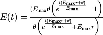
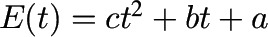Equation for eating rate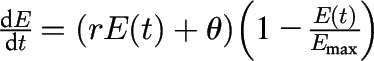
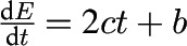Curve shapes?	S-shaped, quadratic, and linear	Quadratic and linear only
Gustatory stimulation phase?	Yes	No, because c < 0. If c is instead chosen to be c > 0, then stimulation is possible; however, then both satiation and maximal food intake can no longer be represented
Satiation phase?	Yes	Yes, assuming c < 0
Maximal food intake represented?	Yes	Yes, only if the x-axis scale is cut off when food intake peaks
Food plateau represented?	Yes	No
Do all predictions make sense?	Yes	No, because 1) a nonzero value of a (fudge factor) means that food has been consumed before the eating episode starts and 2) food intake starts to decline after reaching its maximum value

¹Data are from references 12 and 13. Although the first principles–based model is automatically expressed as a differential equation, the quadratic model can be similarly expressed, which provides a parallel comparison of expressions. e, irrational value of the Euler Constant; E_max, maximal food intake; E(t), amount of food consumed in grams by time in minutes; r, eating duration; θ, nonzero initial eating rate.

How much does the cumulative intake model’s shape vary by participant characteristics?

Because our first-principles model produces a family of curves, the first step is to determine how the 3 key parameters in the model depend on an individual’s characteristics and eating behaviors. This step is different from a goodness-of-fit analysis, which was already performed and discussed by several authors (10, 12), and it is not an examination of physiologic mechanisms. Rather, here we are testing how the shape of the cumulative intake curve varies across subpopulations defined by individual characteristics such as sex, BMI, and age. We did this by performing multivariable linear regression with the 3 eating parameters as dependent variables and with demographic, anthropometric, and eating behavior parameters as independent variables. The full statistical details generated by the linear regression models are provided in Supplemental Table 1.

The optimal model for θ based on participants’ characteristics and eating behaviors produced an adjusted R² of 0.23. Sex (P = 0.002) and the duration of minutes of eating (P = 0.002) were significant, with male sex and longer meal duration associated with higher values of θ. On the other hand, for the parameter r, the best combination of explanatory variables determined the value of r, with an adjusted R² of 0.06; only a tiny portion of the variance in r could be explained by demographic, anthropometric, or eating behavior parameters, which suggests that mean values of r are very similar across subpopulations defined by these characteristics. In fact, sex was the only significant correlate of r (P = 0.03), with female sex associated with higher values of r. Surprisingly, BMI did not influence any of the parameters (Supplemental Table 1). Finally, the equation for E_max yielded an adjusted R² of 0.11. Again, sex was the only significant factor that was associated with E_max (P = 0.012), with male sex associated with higher values of E_max. BMI was borderline significant, at P = 0.08 (Supplemental Table 1). The inclusion of the interaction terms improved the adjusted R² values of 0.26, 0.28, and 0.24 for θ, r, and E_max, respectively. However, none of the interaction terms was significant.

Are individual changes in eating captured by baseline and intervention parameters?

To determine whether changes in eating rates directed through an intervention result in changes in the model parameters, the values of θ, r, and E_max at baseline were compared with their corresponding values in the combined-rate and reduced-rate study interventions. Baseline parameters were all significantly correlated with their reduced-rate parameters (r = 0.50, 0.43, and −0.34) for θ, r, and E_max, respectively. Similarly, baseline parameters were correlated with their combined-rate parameters (r = 0.53, 0.47, and −0.33). The correlation was positive for θ and r and negative for E_max. In addition, baseline θ was positively correlated with E_max (r = 0.73) and negatively correlated with r (r = −0.72). Baseline r was negatively correlated with E_max (r = −0.86). The correlation matrix is shown in Table 3.

TABLE 3.

Pearson correlations between model parameters at baseline and model parameters for the reduced-rate and combined-rate interventions¹

	Baseline
	θ	Emax	r
Baseline
θ	1	0.730	−0.715
Emax	0.730	1	−0.857
r	−0.715	−0.857	1
Reduced rate
θ	0.502	0.425	−0.343
r	−0.438	−0.329	0.300
Emax	0.353	0.286	−0.192
Combined rate
θ	0.533	0.465	−0.328
r	−0.507	−0.511	0.453
Emax	0.359	0.457	−0.318

¹All Pearson correlations were significant, indicating that the individual parameters capture the dynamic eating behavior changes implemented by reducing the eating rates. E_max, maximal food intake; r, eating duration; θ, nonzero initial eating rate.

Description of different eating directives in study 2

There were no differences between the parameter values (θ, r, and E_max) under each directive (“Eat as much as you feel comfortable with” and “Eat as much as you can”). However, the maximal food intake parameter, E_max, was more than double the amount in the groups directed to eat as much as they could (Figure 2A). The eating duration parameter, r, was approximately half the amount in the group directed to eat as much as they felt comfortable with (Figure 2B). Because 1/r represents the time it takes to approximately double the amount of food consumed, a smaller value means it took longer to consume the same amount of food in the group directed to eat as much as they could.

FIGURE 2.

Plots of model simulations calibrated to data from reference 27. Panel A represents unrestrained eaters, and panel B represents restrained eaters. Dashed lines and open circles represent participants who were instructed to eat as much as they could, and solid curved lines and solid circles depict participants who were instructed to eat as much as they felt comfortable with. Values of maximal food intake, E_max, were higher in restrained eaters than in unrestrained eaters. Lower values of r were observed in unrestrained eaters than in restrained eaters. E_max, maximal food intake; r, eating duration; θ, nonzero initial eating rate.

Transition between stimulation and satiation

In the language of mathematics, the inflection point represents the point at which the cumulative intake curve changes concavity from concave up to concave down. In the language of physiology, the inflection point is when eating transitions from the stimulation phase to the satiation phase. We can explicitly compute the timing of the transition by computing the second derivative directly from the following differential equation:

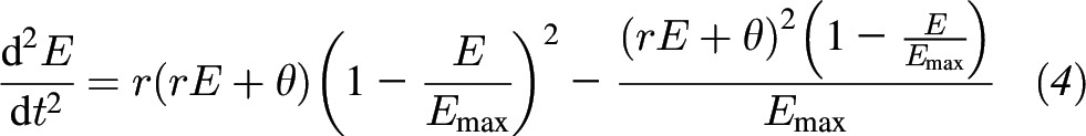Setting the above formula equal to zero and solving for the time yields the following:

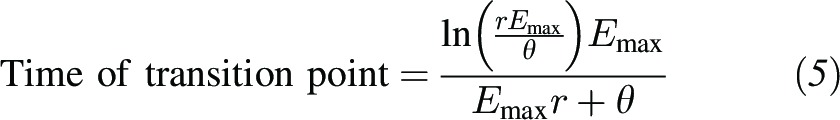The relation between the value transition point and the parameters E_max and r is depicted in the three-dimensional surface plot in Figure 3A. Figure 3A shows that high values of r and E_max increase the timing of the transition point, resulting in a longer stimulation phase. This is exactly what occurred in the subjects who were instructed to eat as much as they could. Conversely, note that high values of r and low values of E_max were observed in the subject who were directed to eat as much as they felt comfortable with, meaning that their stimulation phase was shorter.

FIGURE 3.

A 3-dimensional plot (A) of the time for the transition between stimulation and satiation (i.e., the length of the stimulation phase) compared with E_max and r. The value of θ was set at 50 g/min. (B) The curve that separates the region where transition points exist. Transition points do not occur in the region of low E_max and r. In this region, cumulative intake curves consist only of a satiation phase. (C) A cumulative eating curve simulated from the first-principles model (solid line) with transition point and the simulation and satiation phases identified. The corresponding quadratic model that describes cumulative intake (dashed line) can reflect only the satiation phase because quadratics are limited to exhibiting a single phase with no transition point. E_max, maximal food intake; r, eating duration; θ, nonzero initial eating rate.

Interestingly, the transition point does not exist (Figure 3B) whenever

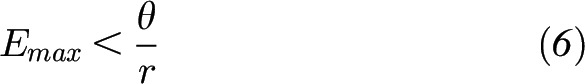What this means is that there are some individuals who experience only satiation but no gustatory stimulation. In the remainder of individuals, there is both a stimulatory phase and a satiation phase (Figure 3C).

DISCUSSION

Cumulative intake curves provide a quantitative description of eating rate and food intake that advances our understanding of eating behaviors and provides opportunities for intervention. Comparing cumulative intake curves between individuals can be achieved by comparing curve shapes and temporal differences in curves. Because this can be challenging, mathematical models with key parameters are needed to model the data (8, 10, 12, 14). Although several such models have been derived that use curve-fitting (10, 12), the first-principles model goes beyond this by satisfying all 4 criteria that define the development of a good model (12, 13). Specifically, the model predicts both gustatory stimulation and satiation, maximal food intake, requires no “fudge factors,” and is self-consistent. Even more importantly, we showed that the model estimated food intake curves better than the quadratic model in 94% of our subjects and improved the quality of fit, as measured by mean SEE scores, by 43%.

To model gustatory stimulation, satiation, and maximal food intake, our first-principles model relied on 3 key parameters that characterize eating behavior: eating duration (r), initial eating rate (θ), and maximal food intake (E_max). Together, these 3 parameters define an individual’s unique cumulative intake curve, which is typically, but not always, S-shaped in form. The “bottom” of the S-shape represents the stimulation phase, whereas the top represents satiation, before reaching a plateau at maximal food intake. We showed how these 3 parameters dictate maximal food intake as well as the balance between stimulation and satiation responses, but also how they can be modified by eating behavior interventions. This latter conclusion was confirmed by correlating baseline and changed parameter values in subjects that purposefully slowed down their eating rates. We also found that this model was similarly able to embody differences in eating behavior on the basis of whether subjects were directed to eat as much as they could or as much as they felt comfortable with (27). Surprisingly, we found that when directed to eat as much as they could, participants consumed nearly twice as much (higher E_max); however, they intrinsically took longer when given this instruction, even when given the same amount of food to eat (lower r).

Interestingly, our investigation uncovered a new finding, that θ is related to E_max, which indicates that the stimulation phase influences eating behavior during the latter portion of the satiation phase. Higher rates of eating during stimulation were associated with a lower maximal intake (E_max). This result means that individuals who eat faster at the beginning of the meal level off their rates of eating at a lower value of E_max (recall that the initial eating rate is not the same as the eating duration). In turn, male sex and longer duration of eating were associated with higher initial eating rates. Interestingly, demographic and anthropometric variables explained only a small fraction of the variance in the 3 key model parameters that completely govern curve shape and form. This suggests that eating behaviors largely depend on other unknown or novel independent factors. This important finding merits further exploration of the factors that determine eating behaviors.

The model also allows investigators and clinicians to compare eating behavior across different subpopulations and under different conditions. By using the model parameters, we showed that the unrestrained group of eaters who were directed to eat as much as they felt comfortable with had different parameter values than those of the group directed to eat as much as they could (27). Overall, this suggests that clinicians could construct eating rate interventions by estimating baseline parameters for the model and then adjust model parameters to generate a new eating curve, which a patient could track to improve their eating behaviors.

This study had several strengths. The presented first-principles model improves on the existing practice of curve-fitting to Universal Eating Monitor data in several ways. First, the model outperforms curve-fitting approaches by incorporating both gustatory stimulation and satiation in the same curve, along with maximal food intake, all while avoiding the use of fudge factors or making nonsensical predictions (e.g., the participant had already started eating before time t=0 min and that cumulative food intake eventually declines). Second, the model outperformed the quadratic model in 94% of our cases. Third, the model presented here can be universally applied to all individuals simply by changing the parameter values. Fourth, the model is valid beyond the observed data, including when food intake has not already reached a plateau, which gives insight into what may happen if the participant is directed to continue eating. The parameters between individuals can be compared with asking important questions. For example, if 2 individuals’ cumulative eating curves yielded different self-limiting maximal food intakes, we can question whether they have different aggregate levels of satiation. Finally, the parameters can be manipulated to design interventions. For example, instead of asking participants to continue to slow down their eating rates by the minute, we can reduce the values of r and θ and the entire dynamic curve will reflect this deceleration. We note that implementing the dynamic curve to guide such progressively slower eating will require a well-designed app and a future pilot study to work out the details.

We have shown that not all cumulative intake curves contain a transition point or, equivalently, both stimulation and satiation. Through the model, we were able to delineate which values of parameters produce curves with only satiation and which produce curves with both stimulation and satiation. Moreover, we were able to explore how changes in the parameters influence the length of the stimulation compared with the satiation phases. For example, such curve changes are observed in rats that were deprived of water (29). Rats that are deprived for longer periods of time exhibit cumulative intake curves with higher values of E_max and r, indicating a longer satiation phase (29). Similarly, rats that were fed food of increasing palatability had higher E_max with a relatively stable r, again indicating a longer satiation phase as well as a higher total food intake (14). Thus, the parameters show not only curve shape and form, but the timing of key events, which could not be determined with the use of earlier models.

This study is not without limitations. We used 2 well-controlled studies that used the validated Universal Eating Monitor to obtain data. However, study 1 was performed in a specific BMI range, and we applied only group mean data from study 2. More data are needed to identify how parameter values may vary by demographic characteristics, food palatability, and other differences and directives. For instance, it may be that there are differences in the quality of the model’s fit in different subpopulations—either better or worse—which would be shown by a wider application of the model. Although these factors, such as sex and BMI, do not represent the underlying physiologic mechanisms, the model still lays the groundwork for predicting risk factors for overeating and for future studies to determine the underlying physiologic mechanisms. In particular, there is a strong need for future studies to measure gastrointestinal peptides such as CCK, mechanical factors such as gastric distention, and psychological factors such as disinhibition, and to pair this with data on daily energy requirements, to better understand the underlying physiologic drivers of food intake and eating rate. This is therefore an important area for future work. Another limitation is that Universal Eating Monitor data are, by necessity, collected in a laboratory setting in which the single, specific meal was consumed in one course. In addition, because Universal Eating Monitor studies are conducted in the laboratory, utensil size, plate size, and cup size did not vary. Thus, research that manipulates the parameters from the first-principles model in free-living conditions and evaluates the effect on food intake is warranted. In addition, for this study, individual parameter calibration is performed manually by using specialized mathematics software. Indeed, before the widespread use of personal computers and the World Wide Web, first-principles models were criticized for being too complex for application (10). However, current models that exhibit even more complexity are easily delivered through computers and smart phones (30). A well-designed, user-friendly app is needed and could automate variable calibrations and deliver informative, graphically pleasing simulations. Although the full implications of the model can be fully determined only after more widespread application, the developed model provides a new method to mechanistically explain and improve model data obtained from Universal Eating Monitors across populations.

REFERENCES

- 1.Kissileff HR, Klingsberg G, Van Itallie TB. Universal Eating Monitor for continuous recording of solid or liquid consumption in man. Am J Physiol 1980;238:R14–22. [DOI] [PubMed] [Google Scholar]
- 2.Kaplan DL. Eating style of obese and nonobese males. Psychosom Med 1980;42:529–38. [DOI] [PubMed] [Google Scholar]
- 3.Kissileff HR, Zimmerli EJ, Torres MI, Devlin MJ, Walsh BT. Effect of eating rate on binge size in bulimia nervosa. Physiol Behav 2008;93:481–5. [DOI] [PMC free article] [PubMed] [Google Scholar]
- 4.Schulz S, Laessle RG. Stress-induced laboratory eating behavior in obese women with binge eating disorder. Appetite 2012;58:457–61. [DOI] [PubMed] [Google Scholar]
- 5.Laessle RG, Lehrke S, Duckers S. Laboratory eating behavior in obesity. Appetite 2007;49:399–404. [DOI] [PubMed] [Google Scholar]
- 6.Martin CK, Anton SD, Walden H, Arnett C, Greenway FL, Williamson DA. Slower eating rate reduces the food intake of men, but not women: implications for behavioral weight control. Behav Res Ther 2007;45:2349–59. [DOI] [PubMed] [Google Scholar]
- 7.Martens MJ, Born JM, Lemmens SG, Karhunen L, Heinecke A, Goebel R, Adam TC, Westerterp-Plantenga MS. Increased sensitivity to food cues in the fasted state and decreased inhibitory control in the satiated state in the overweight. Am J Clin Nutr 2013;97:471–9. [DOI] [PubMed] [Google Scholar]
- 8.Guss JL, Kissileff HR. Microstructural analyses of human ingestive patterns: from description to mechanistic hypotheses. Neurosci Biobehav Rev 2000;24:261–8. [DOI] [PubMed] [Google Scholar]
- 9.Stewart J. Essential calculus: early transcendentals. 2nd ed. Belmont (CA): Brooks/Cole, Cengage Learning; 2013. [Google Scholar]
- 10.Kissileff HR, Thornton J, Becker E. A quadratic equation adequately describes the cumulative food intake curve in man. Appetite 1982;3:255–72. [DOI] [PubMed] [Google Scholar]
- 11.Bobroff EM, Kissileff HR. Effects of changes in palatability on food intake and the cumulative food intake curve in man. Appetite 1986;7:85–96. [DOI] [PubMed] [Google Scholar]
- 12.McCleery RH. On satiation curves. Anim Behav 1977;25:1005–15. [Google Scholar]
- 13.Batzel JJ, Bachar M, Kappel F. Mathematical modeling and validation in physiology: applications to the cardiovascular and respiratory systems. Heidelberg (Germany), New York: Springer; 2013. [Google Scholar]
- 14.Davis JD, Levine MW. A model for the control of ingestion. Psychol Rev 1977;84:379–412. [PubMed] [Google Scholar]
- 15.Kissileff HR, Guss JL, Nolan LJ. What animal research tells us about human eating. In: Meiselman HL, MacFie HJH, editors. Food choice, acceptance, and consumption. New York: Springer US; 1996. p. 105–60. [Google Scholar]
- 16.Kissileff HR, Pi-Sunyer FX, Thornton J, Smith GP. C-terminal octapeptide of cholecystokinin decreases food intake in man. Am J Clin Nutr 1981;34:154–60. [DOI] [PubMed] [Google Scholar]
- 17.Hale JK. Ordinary differential equations. 2nd ed. Huntington (NY): RE Krieger Publishing Co.; 1980. [Google Scholar]
- 18.Vandermeer JH, Goldberg DE; ebrary, Inc. Population ecology first principles. 2nd ed. Princeton (NJ): Princeton University Press, 2013. [Google Scholar]
- 19.Mook DG. Oral and postingestinal determinants of the intake of various solutions in rats with esophageal fistulas. J Comp Physiol Psychol 1963;56:645–59. [Google Scholar]
- 20.Davis JD, Campbell CS. Peripheral control of meal size in the rat: effect of sham feeding on meal size and drinking rate. J Comp Physiol Psychol 1973;83:379–87. [DOI] [PubMed] [Google Scholar]
- 21.Nowlis GH, Kessen W. Human newborns differentiate differing concentrations of sucrose and glucose. Science 1976;191:865–6. [DOI] [PubMed] [Google Scholar]
- 22.Murphy KG, Bloom SR. Gut hormones and the regulation of energy homeostasis. Nature 2006;444:854–9. [DOI] [PubMed] [Google Scholar]
- 23.Kraly FS, Carty WJ, Resnick S, Smith GP. Effect of cholecystokinin on meal size and intermeal interval in the sham-feeding rat. J Comp Physiol Psychol 1978;92:697–707. [DOI] [PubMed] [Google Scholar]
- 24.Verhulst PF. Recherches mathématiques sur la loi d’accroissement de la population. Brussels (Belgium): Nouveaux mémoires de l'Académie Royale des Sciences et Belles Lettres; 1844. [in French]. [Google Scholar]
- 25.Skinner BF. Drive and reflex strength. J Gen Psychol 1932;6:22–47. [Google Scholar]
- 26.Stewart J. Single variable essential calculus: early transcendentals. 2nd ed. Belmont (CA): Cengage Learning, 2012. [Google Scholar]
- 27.Westerterp-Plantenga MS. Eating behavior in humans, characterized by cumulative food intake curves—a review. Neurosci Biobehav Rev 2000;24:239–48. [DOI] [PubMed] [Google Scholar]
- 28.Stunkard AJ, Messick S. The Three-Factor Eating Questionnaire to measure dietary restraint, disinhibition and hunger. J Psychosom Res 1985;29:71–83. [DOI] [PubMed] [Google Scholar]
- 29.Stellar E, Hill JH. The rats rate of drinking as a function of water deprivation. J Comp Physiol Psychol 1952;45:96–102. [DOI] [PubMed] [Google Scholar]
- 30.Martin CK, Gilmore LA, Apolzan JW, Myers CA, Thomas DM, Redman LM. Smartloss: a personalized mobile health intervention for weight management and health promotion. JMIR Mhealth Uhealth 2016;4:e18. [DOI] [PMC free article] [PubMed] [Google Scholar]