Automated Renal Cell Carcinoma Subtype Classification Using Morphological, Textural and Wavelets Based Features

Abstract

We present a new image quantification and classification method for improved pathological diagnosis of human renal cell carcinoma. This method combines different feature extraction methodologies, and is designed to provide consistent clinical results even in the presence of tissue structural heterogeneities and data acquisition variations. The methodologies used for feature extraction include image morphological analysis, wavelet analysis and texture analysis, which are combined to develop a robust classification system based on a simple Bayesian classifier. We have achieved classification accuracies of about 90% with this heterogeneous dataset. The misclassified images are significantly different from the rest of images in their class and therefore cannot be attributed to weakness in the classification system.

1 Introduction

Kidney cancer is one of the leading cancer types in mortality. American Cancer Society estimates that there are about 51,190 new cases of kidney cancer in the United States in the year 2007, and about 12,890 people would die from this disease.

Renal cell carcinoma (RCC) is the most common type of kidney cancer accounting for about 90% of kidney cancers (http://www.cancer.org/docroot/cri/cri_0.asp). RCC usually grows as a single mass within the kidney but sometimes tumors are found at multiple locations and even in both kidneys at the same time. Like other cancers, RCC is difficult to treat when it has metastasized. Thus the key factor in survival lies in early diagnosis. There are several subtypes of RCC, which are primarily classified based on how the cancer cells look under the microscope. The most common subtypes are clear cell RCC, papillary RCC, chromophobe RCC, and renal oncocytoma. These subtypes of RCC are associated with distinct clinical behavior, which makes their classification a critical step before treatment. In addition, to reduce subjectivity and inter-user and intra-user variability, a quantitative approach to RCC classification is urgently needed.

2 Background

Most researchers relied on the traditional pathologist approach of using cellular morphology and tissue structures to classify the images. Considering the heterogeneity in the specimens, and non-standardized image acquisition methods, it is nontrivial to find a solution that is robust and consistently accurate with varying image data sets. Recent trends indicate significant efforts in using quantitative methods to develop automated diagnosis systems for early detection of cancer. Among these systems, a major focus has been directed towards separating cancerous and normal tissue images by classification [1, 2]. Just as in types of cancer diagnosis, in comparing to the normal kidney tissue cells, the renal cancer cells are more irregular with large variations. So it is relatively easier to differentiate cancer tissues from normal tissues, and it is much more challenging to differentiate subtypes of RCC among the cancer tissues.

To improve the classification accuracy, researchers have explored different methodologies with better features. Roula [3] used morphological features for grading of prostate cancer, Thiran [4] used morphological features for classification of cancerous tissues, Diamond [5] and Walker [6] used textural features, Esgiar [1, 7] used fractal analysis and Depeursinge [8] used wavelet frames for classification of lung tissues.

Our previous work [9] for feature extraction used knowledge-based RCC features, selected by expert pathologists and coupled with the priori knowledge about the presence and/or absence of specific histological features, leading to an increase in the classification accuracy. In this paper, we have further improved the classification accuracy for more complex and heterogeneous sets of images. These image sets are specifically selected to evaluate the performance of our classification system.

3 Methods

This study focuses on the classification of RCC pathological images into different subtypes of RCC, which is a more challenging task than separating cancer tissues from normal. Photomicrographs of RCC sections were obtained by using standard pathological procedures. The images were processed to improve the image quality and enhance objects of interest before extracting features. As a first step, color segmentation of these images was used to correct for variations in specimen preparation and image acquisition processes. The resultant images were converted to grayscale images, consistent with the requirement of different types of analysis. In addition, this conversion reduced the computational complexity and resources required for processing. Textural and wavelet analysis of these images was then carried out before extraction of features. Significant features which maximize and highlight the differences among various classes were selected. A set of images pre-classified by an expert pathologist were also processed and the features were stored in a database which was used to train the classification system. Significant features of the test images were compared with the corresponding features in a training database to classify and annotate them accordingly. The following sections describe in detail the image acquisition process, the methods used for image enhancement and color segmentation, morphological, textural and wavelet based feature extraction and the classification system.

3.1 Tissue Specimens and Image Acquisition

All tissues in this study were derived from renal tumors resected by total nephrectomy. Tumors were fixed, processed, sectioned and stained according to standard pathological procedures. Nephrectomy specimens were fixed for at least 1 h in several volumes of 10% neutral buffered formalin, after which representative histologic samples (3-mm thickness) were obtained and fixed overnight in >ten volumes of 10% neutral buffered formalin. Histologic samples were embedded in paraffin and microscopic sections (5-µm thickness) were prepared with a microtome and stained with hematoxylin & eosin. Representative photomicrographs of renal tumor sections were obtained at 200×g total magnification and 1,200 × 1,600 pixels resolution for analysis.

A set of 48 images uniformly distributed in 12 samples from each subclass i.e. clear cell RCC (CC), papillary (PAP), chromophobe RCC (CHR), and renal oncocytoma (ONC) were used for this study. Representative images from each class are shown in Fig. 1. Image data set was created with special emphasis on heterogeneity between the images in each class which can be seen in Fig. 1.

Figure 1.

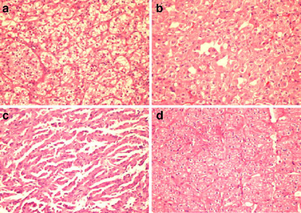
Representative photomicrographs of different types of renal tumor sections stained by hematoxylin & eosin. a clear cell RCC (CC), b chromophobe RCC (CHR), c papillary (PAP), d renal oncocytoma (ONC).

3.2 Color Segmentation

Specimen preparation and image data acquisition involve a number of steps, and these steps are often not standardized or not well controlled. This leads to variations in the image signal intensities and reduces the accuracy of subsequent analysis.

To be consistent with the tissue staining process, the images were transformed to 4-level grayscale images. Our initial approach was to convert the RGB images into a gray-scale intensity image, using the standard perceptual weightings for the three-color components (http://www.poynton.com/notes/colour_and_gamma/ColorFAQ.html#RTFToC11) followed by 4-level quantization. This approach was unsuccessful because of significant intensity variations between the images. Similarly, gray-scale adaptive thresholding produced inconsistent results. K-means, a widely used technique for clustering of multi-spectral data [10] was used for this purpose. The main idea is to define K centroids, one for each cluster. This algorithm aims at minimizing an objective function, a squared error function in this case. The objective function is expressed mathematically as:

$$J={\sum _{j=1}^k\sum _{i=1}^n\Vert x_i^{(j)}-c_j\Vert }^2$$

where ${\Vert x_i^{(j)}-c_j\Vert }^2$ is a distance measure between a data point x(j)i xi(j) and the cluster centre c j, and is an indicator of the distance of the n data points from their respective cluster centers. In this K-means algorithm, each pixel in the image is classified as being part of a cluster. For the case of RCC sub typing, K = 4 clusters are used, corresponding to different regions in the image. Since the result of a K-means algorithm depends on the initial values of cluster centers, we choose the centroids based on the staining colors. The variations from sample to sample are catered by the algorithm by shifting the centroids during the K-means iterative process.

Figure 2 shows a K-means color segmented image. The 4-level grayscale intensity image representation of this color-segmented image as shown in Fig. 2c is used for further analysis.

Figure 2.

Color segmentation results obtained from K-means algorithms. a Original image of ONC b K-means segmented pseudo color image using mean colors c K-means segmented pseudo color image using contrast colors d 4-level grayscale image.

3.3 Morphological, Textural and Wavelet Based Feature Extraction

The 4-level grayscale image is segmented into desired regions of interest. We then analyze images from different RCC subclasses and try to predict the variations in these regions (e.g., the gray level one represents the nuclei in the images). The size of nuclei in one subclass may be different from another subclass, and can be used as one of the differentiating features between the classes. In practice, we may find a feature that differentiates between two subclasses, but this feature may not be useful for other subclasses. This necessitates finding a larger set of features that can differentiate between more subclasses. For this purpose, we have used different methodologies and have combined their results into a set of significant features, which are then used to improve the accuracy of our classification system.

The first method uses gray-level co-occurrence matrix (GLCM), also known as the gray-level spatial dependence matrix (http://www.mathworks.com/access/helpdesk/help/toolbox/images/graycomatrix.html) [11]. Unlike the texture filters, which provide a statistical view of texture based on the image histogram without providing any information about shape, the GLCM method combines textures and morphological statistics into one matrix.

The GLCM is computed by calculating how often a pixel with the intensity (gray-level) value i occurs in a specific spatial relationship to a pixel with the value j. Each element (i, j) in the resulting GLCM is the sum of the number of times that the pixel with value i occurs in the specified spatial relationship to a pixel with value j in the input image.

GLCM computation on our 4-level grayscale images generates a four by four matrix, and an example is shown in Fig. 3. Figure 3a represents a portion of a 4-level gray scale image with elements (1,1), (1,2) and (4,4) indicated for co-occurrence of immediate horizontal neighbors, using an offset mask of [1|1]. Figure 3b shows the corresponding entries in the GLCM using the sum of highlighted elements.

Figure 3.

GLCM computation using 4-level grayscale images. a Representation of 4-level grayscale image b GLCM for highlighted elements in three (a) image.

The gray-level co-occurrence matrix can reveal certain properties about the spatial distribution of the gray levels in the image. For example, if the entries in the GLCM diagonal data are large, the regions are contiguous and the texture is coarse. With a small offset and the large concentrated entries, each diagonal element represents an image area of the corresponding gray-level region of interest. In our implementation, gray-level ‘1’ represents the nuclei, so the GLCM element (1,1) shows the count of total nuclei area in the image in terms of pixels. This count divided by the image size (1,200 × 1,600) gives the normalized nuclei area in the image and is used as one of our desired features.

A few significant features extracted from GLCM are shown in Table 1. CC Clear cell, CHR chromophobe, ONC renal oncocytoma, PAP papillary

Table 1.

Features extracted from GLCM with mean and standard deviations.

	CC	CHR	ONC	PAP
GLCM (1,1)	0.1095 ± 0.0323	0.0608 ± 0.0105	0.0918 ± 0.0289	0.1577 ± 0.0347
GLCM (1,2)	0.0321 ± 0.0079	0.0194 ± 0.0037	0.0285 ± 0.0083	0.0451 ± 0.0083
GLCM (2,2)	0.3988 ± 0.0478	0.5505 ± 0.0628	0.4687 ± 0.1124	0.3614 ± 0.0587
GLCM (2,4)	0.0577 ± 0.0141	0.0547 ± 0.0057	0.0556 ± 0.0242	0.0427 ± 0.0106
GLCM (3,3)	0.0311 ± 0.0459	0.0057 ± 0.0030	0.0217 ± 0.0465	0.0029 ± 0.0039
GLCM (4,4)	0.2613 ± 0.0922	0.2260 ± 0.0763	0.2309 ± 0.0848	0.2943 ± 0.0637

CC Clear cell, CHR chromophobe, ONC renal oncocytoma, PAP papillary

The same GLCMs can be used to derive other statistics about the texture of an image. The most commonly used statistics include:

Contrast—it measures local variations in the gray-level co-occurrence matrix.

$$\sum _{i,j=0}^{N-1}{P}_{i,j}{(i-j)}^2$$

Correlation—it measures the joint probability occurrence of the specified pixel pairs.

$$\sum _{i,j=0}^{N-1}{P}_{i,j}{(i-j)}^2$$

Energy—it is also known as uniformity or the angular second moment, and provides the sum of squared elements in the GLCM.

$$\sum _{i,j=0}^{N-1}{P}_{i,j}^2$$

Homogeneity—it measures the closeness of the distribution of elements in the GLCM to the GLCM diagonal elements.

$$\sum _{i,j=0}^{N-1}\frac{P_{i,j}}{1+{(i-j)}^2}$$

Entropy—it measures the randomness between the elements of GLCM

$$\sum _{i,j=0}^{N-1}{P}_{i,j}(-\text{ln}{P}_{i,j})$$

These textural statistics are computed, and their results are listed in Table 2.

Table 2.

Statistical Features extracted with mean and standard deviations.

	CC	CHR	ONC	PAP
Contrast	0.5712 ± 0.0726	0.4937 ± 0.0492	0.5398 ± 0.2004	0.4592 ± 0.0893
Correlation	0.7496 ± 0.0173	0.7340 ± 0.0610	0.7392 ± 0.0701	0.8252 ± 0.0270
Energy	0.2640 ± 0.0283	0.3759 ± 0.0366	0.3140 ± 0.0778	0.2596 ± 0.0193
Homogeneity	0.8811 ± 0.0069	0.9040 ± 0.0091	0.8885 ± 0.0313	0.8944 ± 0.0148
Entropy	2.3825 ± 0.1960	1.9577 ± 0.0787	2.2077 ± 0.2663	2.3110 ± 0.0639

CC Clear cell, CHR chromophobe, ONC renal oncocytoma, PAP papillary

The use of wavelet transform [12] can also improve feature extraction by performing multi-resolutions analysis of the image. Wavelets are mathematical functions that decompose data into different frequency components, and then study each component with a resolution matched to its scale. Because of its representation of piecewise-smooth signals and fractal behavior owing to its multi-resolution, this method has been successfully used for many biomedical imaging applications [13, 14].

We have used our 4-level grayscale segmented images for wavelet analysis. Biorthogonal wavelet pairs of the third order, a family of B-Splines, are used as the wavelet basis. The discrete wavelet transform of f(x) is given by equations

$$W\phi (j_0,k)=\frac{1}{\sqrt{M}}\sum _{x}f(x){\phi }_{j0,k}(x)$$

$$W\psi (j,k)=\frac{1}{\sqrt{M}}\sum _{x}f(x){\psi }_{j,k}(x)$$

$$\mathit{\text{For}}j\ge j_0\mathit{\text{ and}}$$

$$f(x)=\frac{1}{\sqrt{M}}\sum _k{W}_{\phi }(j_0,k){\phi }_{j0,k}(x)+\frac{1}{\sqrt{M}}\sum _{j-j_0}^{\infty }\sum _k{W}_{\psi }(j,k){\psi }_{j,k}(x)$$

Here f(x), ϕj0, kϕj0, k(x) and ψ j,k (x) are functions of the discrete variable x=0, 1, 2, .., M-1. ϕj0, kϕj0, k(x) and ψ j, k (x) are the scaling and wavelet functions respectively. W ϕ (j 0, k) and W ψ(j,k) are the corresponding scaling (approximation) and wavelet (detail) coefficients. The transformation generates four component sub images, known as Approximation and Detail (Horizontal, Vertical and Diagonal). Figure 4 shows the 4-level discrete wavelet transform (DWT) image, selected sub-images, and the original grayscale image.

Figure 4.

a Four level DWT image, b Level three approximation component, c Level two horizontal detail component, d 4-level grayscale ONC image.

The Wavelet coefficients from the previous stage are processed to enhance the objects of interests. These coefficients contain positive and negative intensities. In post processing, we take the absolute of these intensities and reduce the number of gray levels to four. The remaining analysis of the wavelet images is identical to the process above for four level grayscale images. Each sub image is analyzed using GLCM as well as textural analysis of GLCM by finding properties like contrast, correlation, etc.

Features are computed from four levels of wavelet transform. Every sub image from every level contributes to a large cumulative set of features. These features are ranked based on how well they can discriminate between the RCC images in the training database. Some significant features obtained through the wavelet analysis are listed in Table 3. Once the features of interest are extracted, they are used by the classification system to determine the subtype of cancer image.

Table 3.

Features extracted after DWT with mean and standard deviations.

	CC	CHR	ONC	PAP
GLCM(1,1) (level 1-approx)	0.1072 ± 0.0297	0.0582 ± 0.0109	0.0918 ± 0.0265	0.1601 ± 0.0404
GLCM(1,1) (level 1-diagonal)	0.6327 ± 0.0261	0.6951 ± 0.0383	0.6844 ± 0.0882	0.6915 ± 0.0370
GLCM(1,2) (level 1-diagonal)	0.1122 ± 0.0051	0.0920 ± 0.0089	0.0986 ± 0.0237	0.0988 ± 0.0110
GLCM(2,2) (level 1-horizontal)	0.1260 ± 0.0103	0.1053 ± 0.0116	0.1137 ± 0.0296	0.1080 ± 0.0146
Homogeneity (level 1-vertical)	0.7618 ± 0.0212	0.7976 ± 0.0222	0.7881 ± 0.0629	0.8048 ± 0.0317
Energy (level 1-diagonal)	0.4054 ± 0.0329	0.4874 ± 0.0528	0.4627 ± 0.1131	0.4828 ± 0.0513
Entropy (level 1-horizontal)	0.3941 ± 0.0364	0.4628 ± 0.0476	0.4429 ± 0.1130	0.4677 ± 0.0555
Energy (level 2-diagonal)	0.3221 ± 0.0420	0.3896 ± 0.0534	0.3652 ± 0.1157	0.3969 ± 0.0562

CC Clear cell, CHR chromophobe, ONC renal oncocytoma, PAP papillary

3.4 Classification

Various features extracted from the RCC tissue images using different methodologies are used to classify the subtypes correctly. The analysis of data in Tables 1, 2, and 3 shows that the RCC subtypes have considerable similarities that make it difficult for a single feature to differentiate all the subclasses. This problem can be addressed by increasing the dimensionality and adding more features. As shown by the scatter plot in Fig. 5, the different subclasses can be separated by using three features.

Figure 5.

Scatter plot showing distribution of images for three features: GLCM based energy, GLCM based diagonal component representing cytoplasm area, and wavelet level 1 Diagonal detail GLCM component (2,2); Legend: green circle PAP; red circle CC; blue circle CHR; purple circle ONC.

We have used simple, multi-class Bayes classifier assuming multivariate Gaussian distributions to predict RCC image subclasses. The leave-one-out cross-validation method is used to evaluate the ability of our features and the classifier to correctly predict unknown images. Our results show that by using the features listed in Table 4, our classifier can correctly predict the class of an unidentified sample with an accuracy of 87.5% from our significantly heterogeneous image data. It is interesting to note that most of the misclassified images are significantly different from other images in their own class, thereby contributing to false detection.

Table 4.

List of features selected for the best classification performance with mean and standard deviations.

	CC	CHR	ONC	PAP
GLCM(1,1) (level 1-approx)	0.107 ± 0.0297	0.058 ± 0.0109	0.091 ± 0.0265	0.160 ± 0.0404
GLCM(2,2) (level 1-diagonal)	0.067 ± 0.0031	0.054 ± 0.0060	0.058 ± 0.0200	0.057 ± 0.0083
GLCM(1,1)	0.109 ± 0.0323	0.060 ± 0.0105	0.091 ± 0.0289	0.157 ± 0.0347
GLCM(2,2)	0.398 ± 0.0478	0.550 ± 0.0628	0.468 ± 0.1124	0.361 ± 0.0587
Homo-geneity	0.881 ± 0.0069	0.904 ± 0.0091	0.888 ± 0.0313	0.894 ± 0.0148
Energy	0.264 ± 0.0283	0.375 ± 0.0366	0.314 ± 0.0778	0.259 ± 0.0193

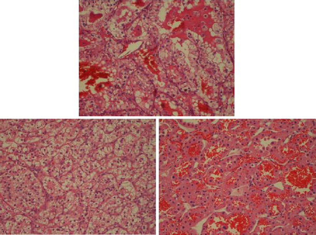
Due to significant difference of these images from other images in their class, some images are misclassified but even the misclassified images are unanimously annotated to one class by most of the features. Figures 6 and 7 shows two examples of the misclassified images along with an image from their correct class as well as an image to the incorrect class to which the image was annotated.

Figure 6.

(Center) PAP image misclassified as ONC. (Left) another PAP image (right) ONC image.

Figure 7.

(Center) CC image misclassified as ONC. (Left) another CC image (right) ONC image.

Although this study showed promising results, much work is still needed towards the eventual goal of a clinical image classification system for routine pathological use.

4 Concluding Remarks

Image features from a single methodology may be good enough for a less varying dataset. But as we increase the complexity and heterogeneity of the images, it becomes difficult to find a set of features that can consistently produce accurate results. By combining features obtained using different methodologies, we show that the feature set becomes more robust and can achieve accurate and consistent results. In addition to improving the feature extraction and classification process, the standardization of tissue sample preparation and the image acquisition process are also important factors. Further, in actual practice the pathologist only concentrates on part of the image and bases his or her classification on the specific region of interest. Manual segmentation of ROI considerably improves the classification accuracy approaching 100% for some datasets. Automatic segmentation of these areas is by itself a problem of considerable complexity. It is thus important to combine these two problems into one system and use areas of high correlation with the training database. Work is ongoing to provide a sophisticated system to assist pathologists in their diagnosis and early cancer detection leading to improved survivability of renal cancer patients.

References

- 1.Esgiar AN, Naguib RNG, Sharif BS, Bennett MK, Murray A. Microscopic image analysis for quantitative measurement and feature identification of normal and cancerous colonic mucosa. IEEE Transactions on Information Technology Biomedicine. 1998;2:197–203. doi: 10.1109/4233.735785. [DOI] [PubMed] [Google Scholar]
- 2.Vermeulena PB, Gasparinib G, Foxc SB, Toid M, Martine L, Mcculloche P, Pezzellaf F, Vialeg G, Weidnerh N, Harrisc AL, Dirix LY. Quantification of angiogenesis in solid human tumors: an international consensus on the methodology and criteria of evaluation. European Journal of Cancer. 1996;32(14):2474–2484. doi: 10.1016/s0959-8049(96)00379-6. [DOI] [PubMed] [Google Scholar]
- 3.Roula MA, Diamond J, Bouridane A, Miller P, Amira A. A multispectral computer vision system for automatic grading of prostatic neoplasia. Proc. IEEE Int. Symp. On Biomed. Imaging. 2002:193–196. [Google Scholar]
- 4.Thiran JP, Macq B. Morphological feature extraction for the classification of digital images of cancerous tissues. IEEE Transactions on Biomedical Engineering. 1996;43(10):1011–1020. doi: 10.1109/10.536902. [DOI] [PubMed] [Google Scholar]
- 5.Diamond J, Anderson N, Bartels P, Montironi R, Hamilton P. The use of morphological characteristics and texture analysis in the identification of tissue composition in prostatic neoplasia. Human Pathology. 2004;35:1121–1131. doi: 10.1016/j.humpath.2004.05.010. [DOI] [PubMed] [Google Scholar]
- 6.Walker RF, Jackway PT, Lovell B, Longstaff ID. Classification of cervical cell nuclei using morphological segmentation and textural feature extraction; Proc of the 2nd Australian and New Zealand Conference on Intelligent Information Systems; 1994. pp. 297–301. [Google Scholar]
- 7.Esgiar AN, Naguib RNG, Sharif BS, Bennett MK, Murray A. Fractal analysis in the detection of colonic cancer images. IEEE Transactions on Information Technology Biomedicine. 2002;6:54–58. doi: 10.1109/4233.992163. [DOI] [PubMed] [Google Scholar]
- 8.Depeursinge A, Sage D, Hidki A, Platon A, Poletti P-A, Unser M, Muller H. Lung Tissue Classification Using Wavelet Frames; 29th Annual International, Conference of the IEEE EMBS; 2007. pp. 6259–6262. [DOI] [PubMed] [Google Scholar]
- 9.Waheed S, Moffitt RA, Chaudry Q, Young AN, Wang MD. Computer Aided Histopathological Classification of Cancer Subtypes. IEEE BIBE. 2007;2007:503–508. [Google Scholar]
- 10.Weeks AR, Hague GE. Color Segmentation in the HSI Color Space Using the k-means Algorithm. Proceedings of the SPIE—Nonlinear Image Processing. 1997;8:143–154. [Google Scholar]
- 11.Hauta-Kasari M, Parkkinen J, Jaaskelainen T. Generalized co-occurrence matrix for multispectral texture analysis. 13th International Conference on Pattern Recognition. 1996;2:785–789. [Google Scholar]
- 12.Arivazhagan S, Ganesan L. Texture classification using wavelet transform. Pattern Recogn Lett. 2003;24(9–10):1513–1521. [Google Scholar]
- 13.Unser M, Aldroubi A. A review of wavelets in biomedical applications. Proceedings of the IEEE. 1996;84(4):626–638. [Google Scholar]
- 14.Fernandez M, Mavilio A. Texture analysis of medical images using the wavelet transform. AIP Conference Proceedings. 2002;630:164–168. October. [Google Scholar]