Concatenated Spatially-localized Random Forests for Hippocampus Labeling in Adult and Infant MR Brain Images

Abstract

Automatic labeling of the hippocampus in brain MR images is highly demanded, as it has played an important role in imaging-based brain studies. However, accurate labeling of the hippocampus is still challenging, partially due to the ambiguous intensity boundary between the hippocampus and surrounding anatomies. In this paper, we propose a concatenated set of spatially-localized random forests for multi-atlas-based hippocampus labeling of adult/infant brain MR images. The contribution in our work is two-fold. First, each forest classifier is trained to label just a specific sub-region of the hippocampus, thus enhancing the labeling accuracy. Second, a novel forest selection strategy is proposed, such that each voxel in the test image can automatically select a set of optimal forests, and then dynamically fuses their respective outputs for determining the final label. Furthermore, we enhance the spatially-localized random forests with the aid of the auto-context strategy. In this way, our proposed learning framework can gradually refine the tentative labeling result for better performance. Experiments show that, regarding the large datasets of both adult and infant brain MR images, our method owns satisfactory scalability by segmenting the hippocampus accurately and efficiently.

1 Introduction

The hippocampus is known as an important brain structure associated with learning and memory [1–4]. The morphological analysis of the hippocampus is a critical step for investigating early brain development [5]. Also, the hippocampus has been found as an early biomarker for many neural diseases including Alzheimer’s disease, schizophrenia, and epilepsy [6, 7]. Therefore, accurate labeling of the hippocampus in Magnetic Resonance (MR) brain images has become a task of pivotal importance to medical image analysis and the related translational medical studies [8, 9].

The automatic methods to accurately and robustly label anatomical regions-of-interest (ROIs) in medical images are highly desirable [10–12]. For example, it often takes up to two hours to manually segment the hippocampus [13], which is infeasible when labeling a large set of subjects. The main challenge in automatic segmentation of the hippocampus is that the intensities in hippocampus are highly similar to those in the surrounding structures, such as amygdala, caudate nucleus, and thalamus [14]. Besides, hippocampal edges are not always visible in the MR images, i.e., a large part of the boundary between the hippocampus and the amygdala is usually invisible [9]. The situation becomes much worse for the cases of infant brain images, where imaging quality is relatively poor with blur intensity boundary between the hippocampus and the surrounding structures [5]. Therefore, it is necessary to utilize prior knowledge for labeling the hippocampus in MR brain images. Note that the prior knowledge here often includes the global position in the brain, the relative position to the neighbor structures, and also the general hippocampus shape [15].

Many automatic labeling methods have been developed to address the above challenges in MR brain segmentation, by learning from the training images and their manually labeled maps, which can be regarded as atlases [16]. There are many different ways of using atlas information for labeling the test images. For example, Carmichael et al. [13] implemented image labeling by first introducing a common atlas that is constructed using a single image [17, 18], or a group of aligned training images [16]. Then, they registered the intensity image of common atlas to the test image, and warped the label map of the common atlas to the test image for segmentation. On the other hand, FreeSurfer toolkit [14] constructed a probability atlas for the whole brain segmentation by applying the label fusion process to a group of images.

Multi-atlas label propagation (MALP) methods have become popular for MR brain labeling recently. The MALP methods intend to use multiple atlases to improve the overall segmentation reliability, compared to the use of a single atlas [19–23]. There are generally two steps in the MALP methods. First, each atlas is spatially aligned to the test image through a certain image registration approach [24–27]. Second, a label fusion method is used to merge the warped atlas labels for final segmentation of the test image. These two steps allow the MALP methods to account for high inter-subject variability between the atlas images and the test image, and produce reliable label estimation for the test image through sophisticated label fusion. Recently, random forest [28–32] has been widely applied to image segmentation [33] and pose recognition [34], and has been proven to be fast and accurate [35]. More detailed literature survey of MALP and the random forest techniques can be found in Section 2.1 and Section 2.3, respectively.

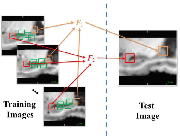
In this paper, we develop a concatenated learning framework that can achieve accurate labeling for the hippocampus in both adult and infant brain images. In particular, we propose to exploit the high variation across different sub-regions of the hippocampus, and then train a set of random forest classifiers specifically for different hippocampal sub-regions. To our best knowledge, there are no existing works that intended to label hippocampal region using the above-described strategy. The main contribution of our method is two-fold. First, each forest is trained for one specific sub-region of the hippocampus, where each sub-region is the ensemble of patches with similar appearances. In the experiments, we have found that, for small ROI such as hippocampus, the patches grouped together with similar appearances are often spatially close to each other. Thus, we can regard that each cluster of patches corresponds to a certain sub-region in the hippocampus, and each trained classifier could have high labeling accuracy for its corresponding sub-region. Second, a novel forest selection strategy is also introduced, such that any voxel in the test image can find its own set of optimal forests to determine the label in the testing stage. Specifically, our forest selection strategy is implemented by comparing the test voxel’s patch with the training patches used to build respective forests. Figure 1 illustrates the main idea of how to implement our spatially-localized random forests. This can also guarantee the scalability of our learning framework, i.e., the forest selection strategy can prevent certain issues when a large set of training atlases are used. Furthermore, we also enhance these spatially-localized random forests by the auto-context strategy [36]. In this way, the higher layer of spatially-localized random forests can extract context features from the outputs of the lower layer of spatially-localized random forests, for helping gradually refine the labeling result for better accuracy.

Figure 1.

Illustration of spatially-localized random forests for hippocampus segmentation. The patches with similar appearances are grouped together to train a specific local classifier, e.g., patches in red are used to train the forest F₁, while patches in orange are used to train F₂. The forest selection strategy is then used to find the optimal forests/classifiers for each voxel in the test image.

The rest of this paper is organized as follows. In Section 2 we survey the literature related to this work, such as the MALP methods, atlas selection, and random forest. In Section 3 we provide details of the proposed spatially-localized random forests for hippocampus segmentation. In Section 4 we demonstrate the segmentation capability of the proposed method on both adult and infant MR brain images, and further compare its performance with the conventional methods. Finally, we conclude our work with discussions in Section 5.

2 Related Works

2.1 The MALP Methods

There are two main directions in the development of the MALP methods, to which the components of registration and label fusion are fundamentally important. For example, to improve the performance in the registration process, Jia et al. [24] proposed the iterative multi-atlas-based multi-image segmentation (MABMIS) approach following a sophisticated tree-based groupwise registration scheme. Wolz et al. [37] introduced the LEAP method which constructed an image manifold to embed all training and test images according to their in-between similarities. The registration task was only implemented between similar training images and test images, such that high labeling reliability could be achieved.

There are also some efforts to improve the component of label fusion in the MALP methods, among which the weighted voting strategy is very popular. The weighted voting strategy often computes the similarities between the training atlas images and the to-be-labeled test image first. The similarities are further considered as weights, which gauge the contributions from individual training atlases to the test image under consideration. As the training atlases with higher weights are more similar to the test image and thus contain more relevant labeling information, the subsequent label fusion process can yield a highly accurate labeling result by fusing the contributions from the atlases adaptively [20, 38–41]. In addition, Warfield et al. [42] introduced the simultaneous truth and performance level estimation (STAPLE) method, which included the expectation-maximization (EM) technique to evaluate the weight information for label fusion.

Another attempt in the development of the MALP methods is the non-local patch-based strategy, which was introduced by Coupé et al. [43] and Rousseau et al. [44]. This strategy has gained momentum due to its capability in quantifying complex variation of image appearances. Inspired by the non-local mean denoising filter [45], the method first extracts small volumetric patches along with their in-between similarities. The segmentation is then implemented by integrating the labels of the non-local voxels in all training atlases, by following their respective patch-based similarities to the voxel under labeling. Since the non-local patch-based labeling does not require precise registration between the training and the testing images, the challenges in the multi-atlas-based segmentation are reduced substantially [43, 46–49]. Various non-local patch-based methods have been developed, including the use of sparsity [50] and label-specific k-NN search structure [48]. Recently, Wu et al. [51] extended the work in [50], where a generative probability model was introduced to segment the test image based on the observations of registered training images. In addition, Asman and Landman [52] improved the STAPLE method by reformulating this statistical fusion method within a non-local mean perspective.

2.2 Atlas selection

As shown in the previous section, the MALP method utilizes the information from multiple atlases to implement the segmentation work. Therefore, its performance is much dependent on the collection of training atlases. First, the computation cost becomes demanding when a large set of training atlases are used, which is often necessary for high labeling accuracy. For example, the current typical non-local label fusion methods require 3–5 hours per single labeling process on a dataset with 15 subjects [52, 53]. The situation becomes worse when the scale of the study becomes larger, such as the Alzheimer’s Disease Neuroimaging Initiative (ADNI) dataset with thousands of subjects. Second, certain atlases can have high appearance/morphological variations with the test image, and thus may contribute misleading information to label the specific test image. The overall labeling performance can be undermined.

To address the aforementioned issues, atlas selection is important. It is shown in Aljabar et al. [19] that the use of atlas selection can significantly improve labeling performance. Generally, the intensity-based similarity (i.e., the sum of squared differences of intensities) or normalized mutual information [54] is used as the metric for atlas selection. Other attempts in atlas selection focus on using the manifold space to embed all images, instead of counting on their Euclidean distances [37, 55]. More references on atlas selection can also be found in Rohlfing et al. [40] and Wu et al. [56].

2.3 Random Forest

The main advantage of using random forest is that it can efficiently handle a large number of images, which is important for MALP image labeling. For example, Zikic et al. [57] intended to apply random forest to automatically label high-grade gliomas from multi-channel MR images. Later they proposed the atlas forest strategy [58], which encoded each individual atlas and its corresponding label map via random forest. Their purpose was to reduce the computational cost, and also to improve the efficiency for experiments, especially when following the leave-one-out validation setting. Experimental results indicated that the performance was favorable compared to the alternatives, e.g., the non-local patch-based method [45, 46].

The major contribution of random forest is its uniform bagging strategy [28], i.e., each tree is trained on a subset of training samples with only a subset of features that are randomly selected from a large feature pool. Thus, the bagging strategy can inject randomness during the learning process, which helps avoid over-fitting and improves robustness of label prediction. However, the drawback of uniform bagging strategy is that each tree is trained using samples from the whole ROIs of all training images. That is, all trees have similar labeling capabilities in general, as their training samples are generated in a similar (though random) way. Since the shapes and the anatomies of different atlas images are quite diverse in the training set, we argue that each tree (or the forest containing multiple trees) can be trained for a specific subset of the atlas information, where the internal anatomical variation is low. In the testing stage, with a proper selection upon the trained classifiers for each test image, the overall labeling performance can be further improved.

Lombaert et al. [59] introduced the Laplacian forest, in which the training images are re-organized and embedded into a low-dimensional manifold. Similar images are thus grouped together. In the training stage, each tree is learned using only a specific group of similar atlases following a guided bagging approach. The strategy for tree selection for the given test image was also proposed. The method was demonstrated experimentally to yield higher training efficiency and segmentation accuracy. However, the Laplacian forest considers only the variability within the entire image space, but neglects the variability across different sub-regions of the ROI (such as hippocampus). For the case of the hippocampus segmentation, the target region is small, compared to the whole brain image. Therefore, the global differences between whole brain images do not represent the shape differences of the hippocampus across subjects, thus making it hard to select the optimal forests/classifiers for hippocampus segmentation in the test image.

3 Methods

In this section, we propose a concatenated spatially-localized learning framework, based on random forests, to address the variation of appearances across different sub-regions of the hippocampus in the MR brain images. In particular, we train a set of spatially-localized random forests for targeting different sub-regions of the hippocampus. Then, in the application stage, each voxel in the test image selects a subset of optimal forests/classifiers for determining its label. To further improve the labeling performance, we further iteratively enhance each spatially-localized random forest with the auto-context strategy [36]. In this concatenated learning framework, we construct the higher layer of spatially-localized random forests by also partially using the outputs of their respective forests in the lower layer. As the layer increases, the labeling results can be gradually refined.

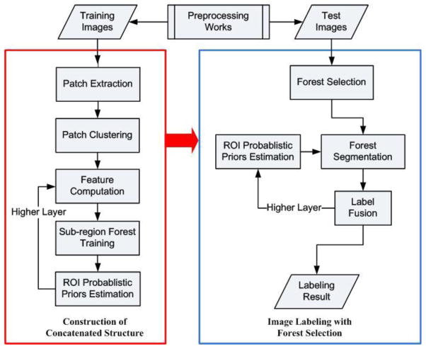
Figure 2 presents the flowchart of the proposed framework, which consists of the training and the testing stages. The details of the algorithm in all steps are given in the subsequent sections. In the training stage, we commence by implementing the 3D cubic patch extraction from the training atlases in the bottom layer, as detailed in Section 3.1. Then, voxels with similar patch-based appearances are clustered together. Next, we consider all patches in the same cluster to form a specific sub-region. Note that the shapes of the same sub-region might vary across different training atlases. The strategy of patch clustering is detailed in Section 3.2.

Figure 2.

Schematic illustration of the proposed hippocampus segmentation framework, which consists of the training stage (in red) and the testing stage (in blue).

With the partition of sub-regions, we then randomly select voxel samples from the training atlases. Their features are computed accordingly. The strategy of feature computation is detailed in Section 3.3. As stated previously, each random forest is trained by using only samples extracted from its corresponding sub-region in all the training atlases. The forest training process generally follows the standard random forest technique with details in Section 3.4.

In the layers upper than the bottom one, the sub-regions are identical to those decided early. However, by following the auto-context strategy, the classifiers in the second layer and above are trained using not only the visual features from the original intensity images but also the context features extracted from the outputs of the lower-layer classifiers. The feature extraction of both visual and context features is also detailed in Section 3.3.

In the testing stage, for each voxel in the test image, we first extract the corresponding patch centered at the test voxel. Then, we implement a forest selection strategy to find a subset of classifiers that are the most appropriate to label the test voxel under consideration. By following the trained hierarchy, the labeling results are gradually refined through all layers. The output of the upmost layer gives the labeling result for the specific test voxel under consideration. Details of the segmentation process with the forest selection technique are presented in Section 3.5.

3.1 Patch Extraction

In the training stage, we commence by randomly extracting numerous patches from all the training atlases. Denote the training atlas set as A, which consists of n atlases {A_i = (I_i, L_i)|i = 1,...,n}. Each atlas such as the i-th atlas A_i includes an intensity image I_i and a label image L_i. In each intensity image, we select m patches. Thus, the total number of the 3D patches is m × n. The set of patches is denoted as P = {p₁, p₂,...,p_m×n}.

There are several restrictions in the patch extraction process. First, the extracted patches should reflect the common appearance as well as the variation in the neighborhood of the targeting ROI. Therefore, the locations of patches are not selected from the whole brain image, but only from a small region that covers the hippocampus with certain margins. Second, we assign higher priority for choosing patches close to the hippocampal boundaries. In this way, we can get more boundary information from the selected patches. Third, large overlapping between any pair of selected patches should be avoided. Otherwise, the selected patches will contain highly-redundant information, which may affect the subsequent learning process.

To meet the above restrictions during the patch extraction process, we adopt the importance sampling strategy [60]. That is, we first extract the hippocampal boundaries in each training atlas and then smooth boundaries with a Gaussian kernel. The resulted probability map records the importance of individual voxels/patches to be selected for training, as the voxels closer to the hippocampal boundaries are more likely to be selected. Also, when a certain patch is chosen, the corresponding patch in the probability map will be marked and the respective probability values will be reduced. This adjustment can reduce the chance of selecting future patches in the neighborhood, thus preventing large overlap between extracted patches.

3.2 Patch Clustering

Next, we cluster the selected patches to determine the partition of the sub-regions. The clustering process is based on the intensity similarity between patches, defined by the mean of squared intensity differences as below, i.e., for two patches p_i and p_j:

$$S(p_i,p_j)=-{\Vert p_i(x)-p_{\mathrm{j}}(x)\Vert }^2,$$ (1)

where x is the voxel in p_i and p_j. When similarities between all pairs of patches are obtained, we can obtain an (m × n) × (m × n) affinity matrix. The patches can then be clustered and used to determine sub-regions that correspond to respective clusters. Specifically, we choose the affinity propagation method [61] for clustering the extracted patches as it can automatically find the number of clusters given the input affinity matrix.

The affinity propagation method follows an iterative strategy to find the optimal exemplar nodes (corresponding to certain extracted patches) that best represent the overall data points. Then the exemplars are used as the representatives for their corresponding clusters. The affinity propagation method commences by initializing a preference value for each node in the affinity matrix, regarded as its likelihood of being chosen as the exemplar. State succinctly, all nodes in the initialization step are assumed to be exemplar candidates. In each iteration, the affinity propagation method intends to pass two messages between the exemplar candidates and other nodes, namely the responsibility and the availability. The clustering process finishes when all messages are converged to be fixed, as several exemplars are selected to represent individual clusters in the final. Details of the affinity propagation method can be found in Frey and Dueck [61]. When similar patches are grouped together, each cluster can be used to train its own forest, which can be then used for labeling the specific sub-region in the test image.

3.3 Haar-like Feature Computation

Given numerous voxel samples that are randomly selected from the training atlases, we need compute their corresponding features before training the classifiers. The numbers of samples extracted from different training atlases are generally identical. In the bottom layer, only the 3D Haar-like visual features are computed from the intensity images. In the second and upper layers, both visual features and context features are computed. Note that the context features are computed from the output maps of the lower-layer forests. We will later introduce the strategy to obtain the segmentation outputs from a certain layer in our concatenated learning framework (c.f. in Section 3.5). Visual features and context features are computed from two different sources in the set Q = {Q₁, Q₂}. By following the auto-context strategy, we combine these two different types of features together to train the classifiers. It is worth noting that the numbers of features extracted from the two sources are the same, implying that these two types of features are treated equally in our implementation.

In this paper, we apply the 3D Haar-like operators to extract visual and context features due to the computational efficiency and simplicity [62]. For the cubic region R centered at sampled voxel x, we randomly sample two cubic areas R₁ and R₂ that are within R. State succinctly, the sizes of the cubic regions are randomly chosen from an arbitrary range, which in our work is {1,3,5} in voxels. We follow two ways to compute the Haar-like features: (1) the local mean intensity in R₁, or (2) the difference of local mean intensity in R₁ and R₂ [63]. The Haar-like feature operator can be thus given as follows [64]:

$$f_{\text{Harr}}(x,Q_i)=\frac{1}{\mid R_1\mid }{\sum }_{u\in R_1}{Q}_i(u)-\delta \frac{1}{\mid R_2\mid }{\sum }_{v\in R_2}{Q}_i(v),R_1\subseteq R,R_2\subseteq R,\delta \in \{0,1\},$$ (2)

where f_Harr(x, I_i) is a Haar-like feature for the voxel x in the source data Q_i, and the parameter δ is 0 or 1 which is used to determine the selection of one or two cubic regions. Note that the parameter values described above are randomly decided during the training stage, which are stored for future use in the testing stage. In this way, we can avoid the costly computation of the entire feature pool and then sample features from the pool efficiently.

3.4 Forest Training

In this section, we present details on training the forest for patch labeling by using the features obtained in Section 3.3. As stated in Section 2.3, the random forest F is an ensemble of b binary decision trees {T₁,T₂,...,T_b}. In each tree, only a subset of features and samples are selected for training. It is worth noting that all trees belonging to the same forest are trained using an identical set of samples in our work due to computation simplicity. Also note that the strategy for training the classifier is irrelevant whether the context features are included in the input samples. Therefore, the following descriptions of classifier training also apply to both the forests in the bottom and the upper layers of the hierarchy.

The binary decision tree is a tree-structured classifier containing two types of nodes, i.e., the internal node and the leaf node [31]. Every internal node has a split function to divide the training sets into its left or right child node based on one feature and its threshold setting. The split function intends to maximize the information gain of splitting the training data [28]. On the other hand, the leaf nodes store the hippocampus label predictor.

In the training stage, given an input voxel sample x, the decision tree T_i can produce a label predictor g(h|f(x, Q),T_i). Here, h is the hippocampus label, and f(x, Q) is the high-dimensional Haar-like feature vector computed from the source set Q in Section 3.3. The tree is trained as follows: We commence by constructing its root (internal) node, where its split function is optimized to split the training samples into two subsets, which are then placed in the left and right children (internal) nodes. The settings for the optimal split function are stored for future use in the testing stage. Next, the tree keeps growing by recursively computing the split function in each of the child (internal) nodes and further dividing the samples, until either the maximum tree depth is reached, or the number of training samples belonging to the internal node is too small to divide. Here, the leaf nodes are appended, whose probability results are computed by first counting the labels of all training samples in each leaf node l and then associating it with the empirical distribution over its label predictor g_l(h|f(x,Q),T_i) [64].

3.5 Forest Selection and Fusion

In the testing stage, for each to-be-labeled voxel x in the test image I′, we first follow the forest selection strategy to find a subset of optimal forests/classifiers trained for different sub-regions. Then, each selected classifier is applied to produce a probability value, and results of all selected classifiers are merged to give the final estimation for the test voxel x.

The strategy of forest selection is presented as follows. As mentioned in Section 3.1, the set of patches collected from all the training images is P = {p₁, p₂,...,p_m×n}. We commence by extracting the patch p_x centered at the voxel x from the test image I′. Then, we compare the patch p_x with those in P by using Equation (1), and obtain a corresponding set of comparison results S_x = {s₁, s₂,...,s_m×n}. Next, we select a group of the patches P_x ⊂ P whose values in S_x are highest. After patch clustering process introduced in Section 3.2, each sub-region has its corresponding set of patches $P^i=\{p_1^i,p_2^i,\dots ,p_{m_i}^i\}$. The novel metric W(x, Pⁱ) for the test voxel x is thus given as follows:

$$W\left(x,P^i\right)=\frac{|P_x\cap P^i|}{\left|P^i\right|},$$ (3)

where |·| calculates the size of the set. When the clusters with top W scores are selected, the set of their corresponding trained forests can be chosen to label the test voxel x. Denote the set of selected forests as F = {F₁, F₂,...,F_q}, the strategy of label fusion is given as follows. We commence by estimating the probability results from all the trained trees { $T_1^j,T_2^j,\dots ,T_b^j$} in each forest F_j. The test voxel x is first pushed separately into their root (internal) nodes. Guided by the learned splitting functions in the training stage, for each tree $T_i^j$ the voxel arrives at a certain leaf node, and the corresponding probability result is thus obtained as $g(h\mid \mathit{f}(x,\mathit{Q}),T_i^j)$. The overall probability from the spatially-localized forest $F_j^k$ can be estimated by averaging the obtained probability results from all the trees, i.e.,

$$g(h\mid x,F_j)=\frac{1}{b}{\sum }_{i=1}^{b}g(h\mid \mathit{f}(x,\mathit{Q}),T_i^j).$$ (4)

The final estimation can be measured by implementing a weighted averaging of the produced probability values, where the weight is given by the score value W. The equation is written as:

$$g(h\mid x)={\sum }_{i=1}^q\frac{W(x,P^i)g(h\mid x,F_i)}{W(x,P^i)}.$$ (5)

4 Experiments

In this section, we evaluate the proposed framework in labeling the hippocampus from MR brain images. We use two datasets, including (1) some selected images from Alzheimer’s Disease Neuroimaging Initiative (ADNI)¹ [65] and (2) the infant brain images. Our experiments aim to demonstrate the validity of proposed framework in both adult and infant brain images, respectively.

We perform cross-validation to both datasets, to show the robustness of the proposed framework. It is also worth noting that the settings for the classifier training and testing are generally identical in all the experiments. Specifically, there are 20 trees trained in each random forest. The maximum tree depth is 20. Each leaf node has a minimum of 8 samples. The number of 3D Haar-like features used for each tree is 2000, which include both visual and context features. The size of the cubic region used to compute Haar-like features is 11mm ×11mm×11mm. Also, in the patch extraction process described in Section 3.1, we extract 150 patches from each training image. In the patch clustering process, the preference parameter for affinity propagation method is set by following the recommendance in [61]. In the testing stage, for each voxel in the test image, we set that only 22% of the forests (with the highest W scores) are selected for segmentation. Experiments show that the configurations presented above can produce reliable labeling results for both datasets.

We used the standard preprocessing procedure to both ADNI and infant images, by following [43] to ensure the validity of the estimation. Besides, the ITK¹-based histogram matching program was also applied to both data independently. All images were rescaled to the intensity range [0, 255]. To reduce the computational complexity, for each input testing image, only the masked region is considered for labeling. To acquire the mask, we first register all the label maps in the training atlases to the space of the testing image, and then compute the union of all the warped label maps as the mask. It has proven in the experiment that the obtained mask can completely cover the entire hippocampus ROI for further estimation.

Note that we have constructed the three-layer hierarchy for experiments of both ADNI and infant datasets. This is determined by balancing between the overall labeling accuracy and time cost. Experiments also show that the three-layer hierarchy yields satisfactory results.

4.1 ADNI Dataset

The first experiment is to apply the proposed framework to the ADNI dataset which provides a large number of adult brain MR images, along with the annotated left and right hippocampi [65]. We have randomly selected 64 ADNI images from the normal control (NC), mild cognitive impairment (MCI), and Alzheimer’s disease (AD) groups of subjects. Here we applied 8-fold cross validation to evaluate the validity of the propose framework. State succinctly, the 64 images are equally divided into 8 folds. In each fold, we select one fold for testing, and the rest for training. Note that the numbers of the selected test images in each fold are generally identical for the three subject groups (NC, MCI, and AD).

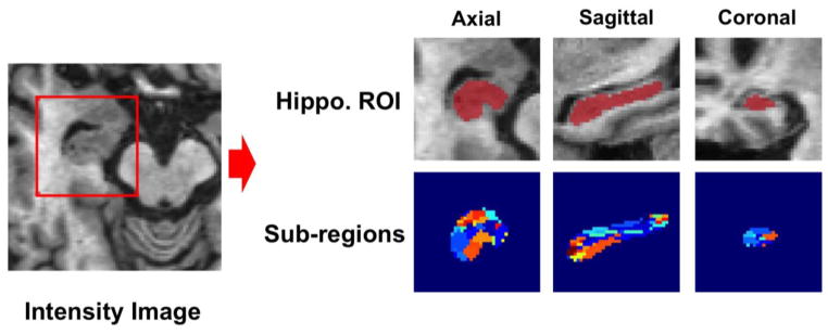
Our goal in this section is to demonstrate the hippocampus labeling performance by our concatenated spatially-localized random forest framework. Figure 3 shows one example of the sub-region distribution for the left hippocampi in the ADNI dataset. Note that the union of the sub-regions is equal to the mask region generated in the preprocessing procedure. It can be observed that each sub-region, denoted by different color in the figure, occupies a respective part of the hippocampal ROI. Therefore, this partition fits our settings for the proposed spatially-localized random forest. Table 1 presents the comparison results between the labeling estimates and the groundtruth with the Dice similarity coefficient (DSC) [66]. The first column shows the labeling performance when applying the conventional random forest technique. The second column shows the results of the sub-region random forest, without using auto-context strategy. The third and the fourth columns show the performances when applying two and three layers of the sub-region random forests, respectively.

Figure 3.

The sub-regions (represented by different colors) established for the left hippocampi in the ADNI dataset. Note that the union of these sub-regions is equal to the mask generated in the pre-processing procedure.

Table 1.

Quantitative comparison of performances in different configurations when labeling the left and the right hippocampi.

	Conventional Random Forest	Sub-Region Random Forest
		First Layer	Second Layer	Third Layer
Left Hippo.	84.71±3.48%	85.82±2.47%	86.89±2.36%	87.01±2.28%
Right Hippo.	83.83±4.01%	85.29±2.82%	86.29±2.74%	86.45±2.73%
Overall	84.27±3.75%	85.56±2.65%	86.59±2.55%	86.73±2.51%

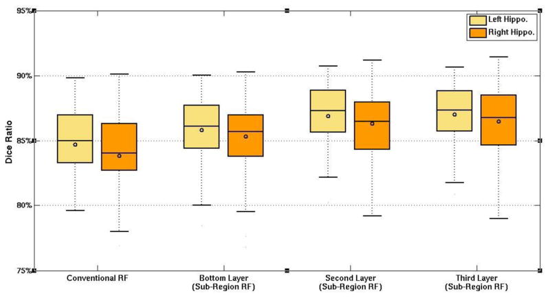
Figure 4 presents the box plots to visualize the performances of the three layers, by comparion with the conventional random forest method. The left and the right panels correspond to the results of the left and the right hippocampi, respectively.

Figure 4.

The box plot for the labeling accuracies of different configurations on the left (yellow) and the right (orange) hippocampi from the ADNI dataset. RF is short for random forest.

It can be observed that the DSC scores of the higher layer are better than those of the lower layers in both hippocampi. Meanwhile, the proposed method is clearly better than the conventioal random forest technique. Particularlly, the labeling performance in the top layer of the hierarchy has overall 2.46% improvement than the conventaionl random forest technique. It is also worth noting that the p-values in the two-tailed paired t-tests between any two layers for both the left and the right hippocampi are below 0.05, indicating the statistical significant improvement of the proposed framework in labeling the hippocampus from adult MR brain images.

Note that when more layers are constructed, the labeling performance converges gradually. This property can also be observed in other works using auto-context strategy [67]. It is also worth noting that the average runtime of the labeling process using one layer of the hierarchy is ~10 minutes using a standard computer (Intel Core i7-4770K 3.50GHz, 16GB RAM). When all three layers are used, it takes 27 minutes as the test image goes through the entire hierarchy for its final segmentation in our experiment. Note that the comparable runtime performances can also be observed when labeling the infant images, as presented in the next section.

4.2 Infant Dataset

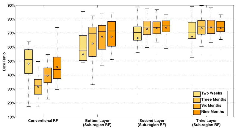
In this experiment, we focus on applying the proposed framework to the infant MR brain images. The infant images were acquired from a Siemens head-only 3T scanner. There are 10 subjects participated in the acquisition, each of which has been scanned at 2 weeks, 3 months, 6 months, and 9 months of the age, respectively. Here, the images acquired in the same time point are considered as one dataset, since the appearance diversity across different time points is much higher than that across different subjects. The images were acquired with 144 sagittal slices using the following parameters: TR/TE = 1900/4.38ms, flip angle = 150 degrees, resolution=1×1×1mm.

Within each dataset of a specific time point, we adopt the leave-one-out setting due to the limited image number. Table 2 shows the comparison results between the estimated labeling results and the groundtruth using the DSC. The four rows in the table represent the results of four different time points. Also, Figure 5 shows the box plots to compare the detailed performances of the proposed framework (with different configurations) and the conventional random forest method. Due to the challenges of labeling the hippocampus for infant MR brain images as introduced in Section 1, the performance is quite limited using the conventional random forest technique. For example, the overall DSC is only 41.22% in DSC for four time points. However, it can also be observed that the proposed framework can effectively overcome the challanges, as the performance has been greatly improved (>30% increase in DSC). This demonstrates the validity of the proposed framework when applied to the infant brain images. Also note that the difference between results obtained by the conventional random forest method and the proposed method is statistically significant, with the p-values in the two-tailed paired t-tests all below 0.05 for the images at each of four scanning time points.

Table 2.

Quantitative comparison of performances in different configurations when labeling the left and the right hippocampi.

	Conventional Random Forest	Sub-Region Random Forest
		First Layer	Second Layer	Third Layer
Two Weeks	48.02±11.61%	54.74±17.11%	66.48±14.31%	67.40±14.18%
Three Months	31.63±8.17%	62.52±16.26%	72.65±8.15%	73.31±7.64%
Six Months	39.43±7.58%	67.44±9.78%	73.58±7.69%	74.01±8.12%
Nine Months	45.79±11.40%	67.39±9.74%	73.91±5.67%	73.50±5.84%
Overall	41.22±9.69%	63.02±13.22%	71.66±8.96%	72.06±8.95%

Figure 5.

The box plot for the labeling accuracies of the hippocampus on infant MR brain images of four time points.

There are also alternative methods that focuse on hippocampus labeling of the infant brain images, such as the unsupervised deep learning framework proposed by Guo et al. [5]. By using the same infant dataset, the hippocampus segmentation results are reported to be 70.2% in DSC in average. It can therefore be concluded that the proposed framework can generally outperform the state-of-the-art methods when labeling the hippocampus in infant MR brain images.

5 Conclusion

In this paper, we present a novel concatenated learning framework for hippocampus labeling in both adult and infant MR brain images. We propose training spatially-localized random forests for specific sub-regions of the hippocampus to achieve better segmentation. In the testing stage, we also apply a novel forest selection for each voxel in the test image, such that the test voxel can fuse its label by using the outputs of the selected optimal random forests. We further iteratively enhance the proposed spatially-localized random forest by following the auto-context strategy. This concatenated framework allows the tentative labeling results to be gradually refined, until reaching satisfactory segmentation results in the last layer.

In the experiments, we demonstrate the performances of the proposed framework on both adult and infant brain MR images. We construct a three-layer framework for our method, and compare its labeling performances (from different layers) with the conventional method. Our results show that our proposed framework can achieve significant improvement in hippocampus labeling, and also owns satisfactory scalability when applied to the datasets with large set of atlas images In the future work, we will extend the proposed framework to support multi-ROI labeling and apply it to whole brain segmentation.

Biographies

Lichi Zhang received the BE degree from the School of Computer Science, Beijing University of Posts and Telecommunications, China in 2008, and the PhD degree from Department of Computer Science, University of York, UK, in 2014. He is now a postdoc researcher in Med-X research Institute, Shanghai JiaoTong University, China. His research interests include 3D shape reconstruction, object reflectance estimation and medical image analysis.

Qian Wang received the BE degree from the Department of Electronic Engineering, Shanghai JiaoTong University, China, in 2006, the MSc degree from the Department of Electronic Engineering, Shanghai JiaoTong University, China, in 2009. In 2013, he completed a PhD degree in University of North Carolina at Chapel Hill (UNC-CH), North Caroline. He is now a research scientist in Med-X research Institute, Shanghai JiaoTong University, China. His research interests include temporal/longitudinal image analysis, quantitative image analysis, image enhancement and translational medical study.

Yaozong Gao received the BE degree from the Department of Software Engineering, Zhejiang University, China, in 2008, and the MSc degree from the Department of Computer Science, Zhejiang University, China, in 2011. He is currently working toward the PhD degree in the Department of Computer Science, University of North Carolina at Chapel Hill (UNC-CH), North Carolina. Since fall 2011, he has been with the Department of Computer Science, the Department of Radiology, and Biomedical Research Imaging Center (BRIC), UNC-CH. His research interests include machine learning, computer vision, and medical image analysis.

Guorong Wu is an assistant professor in Radiology, Biomedical Research Imaging Center (BRIC), Computer Science, and Biomedical Engineering in the University of North Carolina at Chapel Hill (UNCCH). He has been working on medical image registration since 2003, and have developed more than 10 registration methods for brain magnetic resonance imaging (MRI), diffusion tensor imaging (DTI), breast dynamic contrast enhanced MRI (DCE-MRI), and lung 4D computer tomography (CT) images. His research interests include large population data analysis, computer assisted diagnosis and image guided radiation therapy.

Dinggang Shen is a professor in Radiology, Biomedical Research Imaging Center (BRIC), Computer Science, and Biomedical Engineering in the University of North Carolina at Chapel Hill (UNCCH). He is currently directing the Center for Image Informatics, the Image Display, Enhancement, and Analysis (IDEA) Lab in the Department of Radiology, and also the medical image analysis core in the BRIC. He was a tenure-track assistant professor in the University of Pennsylvanian (UPenn), and a faculty member in the Johns Hopkins University. His research interests include medical image analysis, computer vision, and pattern recognition. He has published more than 500 papers in the international journals and conference proceedings. He serves as an editorial board member for six international journals. He also serves in the Board of Directors, The Medical Image Computing and Computer Assisted Intervention (MICCAI) Society.

References

- 1.den Heijer T, van der Lijn F, Vernooij MW, de Groot M, Koudstaal P, van der Lugt A, Krestin GP, Hofman A, Niessen WJ, Breteler MM. Structural and diffusion MRI measures of the hippocampus and memory performance. Neuroimage. 2012;63:1782–1789. doi: 10.1016/j.neuroimage.2012.08.067. [DOI] [PubMed] [Google Scholar]
- 2.Jeneson A, Squire LR. Working memory, long-term memory, and medial temporal lobe function. Learning & Memory. 2012;19:15–25. doi: 10.1101/lm.024018.111. [DOI] [PMC free article] [PubMed] [Google Scholar]
- 3.Scoville WB, Milner B. Loss of recent memory after bilateral hippocampal lesions. Journal of neurology, neurosurgery, and psychiatry. 1957;20:11. doi: 10.1136/jnnp.20.1.11. [DOI] [PMC free article] [PubMed] [Google Scholar]
- 4.Wixted JT, Squire LR. The medial temporal lobe and the attributes of memory. Trends in cognitive sciences. 2011;15:210–217. doi: 10.1016/j.tics.2011.03.005. [DOI] [PMC free article] [PubMed] [Google Scholar]
- 5.Guo Y, Wu G, Commander LA, Szary S, Jewells V, Lin W, Shen D. Medical Image Computing and Computer-Assisted Intervention MICCAI 2014. Springer; 2014. Segmenting Hippocampus from Infant Brains by Sparse Patch Matching with Deep-Learned Features; pp. 308–315. [DOI] [PMC free article] [PubMed] [Google Scholar]
- 6.Van Leemput K, Bakkour A, Benner T, Wiggins G, Wald LL, Augustinack J, Dickerson BC, Golland P, Fischl B. Automated segmentation of hippocampal subfields from ultra-high resolution in vivo MRI. Hippocampus. 2009;19:549–557. doi: 10.1002/hipo.20615. [DOI] [PMC free article] [PubMed] [Google Scholar]
- 7.Convit A, De Leon M, Tarshish C, De Santi S, Tsui W, Rusinek H, George A. Specific hippocampal volume reductions in individuals at risk for Alzheimer’s disease. Neurobiology of aging. 1997;18:131–138. doi: 10.1016/s0197-4580(97)00001-8. [DOI] [PubMed] [Google Scholar]
- 8.Gousias IS, Edwards AD, Rutherford MA, Counsell SJ, Hajnal JV, Rueckert D, Hammers A. Magnetic resonance imaging of the newborn brain: manual segmentation of labelled atlases in term-born and preterm infants. Neuroimage. 2012;62:1499–1509. doi: 10.1016/j.neuroimage.2012.05.083. [DOI] [PubMed] [Google Scholar]
- 9.Dill V, Franco AR, Pinho MS. Automated Methods for Hippocampus Segmentation: the Evolution and a Review of the State of the Art. Neuroinformatics. 2014:1–18. doi: 10.1007/s12021-014-9243-4. [DOI] [PubMed] [Google Scholar]
- 10.Xia Y, Ji Z, Zhang Y. Brain MRI image segmentation based on learning local variational Gaussian mixture models. Neurocomputing. 2016 [Google Scholar]
- 11.Dai S, Lu K, Dong J, Zhang Y, Chen Y. A novel approach of lung segmentation on chest CT images using graph cuts. Neurocomputing. 2015;168:799–807. [Google Scholar]
- 12.Ji Z, Xia Y, Sun Q, Chen Q, Feng D. Adaptive scale fuzzy local Gaussian mixture model for brain MR image segmentation. Neurocomputing. 2014;134:60–69. doi: 10.1109/TITB.2012.2185852. [DOI] [PubMed] [Google Scholar]
- 13.Carmichael OT, Aizenstein HA, Davis SW, Becker JT, Thompson PM, Meltzer CC, Liu Y. Atlas-based hippocampus segmentation in Alzheimer’s disease and mild cognitive impairment. Neuroimage. 2005;27:979–990. doi: 10.1016/j.neuroimage.2005.05.005. [DOI] [PMC free article] [PubMed] [Google Scholar]
- 14.Fischl B, Salat DH, Busa E, Albert M, Dieterich M, Haselgrove C, Van Der Kouwe A, Killiany R, Kennedy D, Klaveness S. Whole brain segmentation: automated labeling of neuroanatomical structures in the human brain. Neuron. 2002;33:341–355. doi: 10.1016/s0896-6273(02)00569-x. [DOI] [PubMed] [Google Scholar]
- 15.van der Lijn F, den Heijer T, Breteler MM, Niessen WJ. Hippocampus segmentation in MR images using atlas registration, voxel classification, and graph cuts. Neuroimage. 2008;43:708–720. doi: 10.1016/j.neuroimage.2008.07.058. [DOI] [PubMed] [Google Scholar]
- 16.Kuklisova-Murgasova M, Aljabar P, Srinivasan L, Counsell SJ, Doria V, Serag A, Gousias IS, Boardman JP, Rutherford MA, Edwards AD. A dynamic 4D probabilistic atlas of the developing brain. NeuroImage. 2011;54:2750–2763. doi: 10.1016/j.neuroimage.2010.10.019. [DOI] [PubMed] [Google Scholar]
- 17.Chakravarty MM, Sadikot AF, Germann J, Bertrand G, Collins DL. Towards a validation of atlas warping techniques. Medical image analysis. 2008;12:713–726. doi: 10.1016/j.media.2008.04.003. [DOI] [PubMed] [Google Scholar]
- 18.Chakravarty MM, Sadikot AF, Germann J, Hellier P, Bertrand G, Collins DL. Comparison of piece-wise linear, linear, and nonlinear atlas-to-patient warping techniques: Analysis of the labeling of subcortical nuclei for functional neurosurgical applications. Human brain mapping. 2009;30:3574–3595. doi: 10.1002/hbm.20780. [DOI] [PMC free article] [PubMed] [Google Scholar]
- 19.Aljabar P, Heckemann RA, Hammers A, Hajnal JV, Rueckert D. Multi-atlas based segmentation of brain images: atlas selection and its effect on accuracy. Neuroimage. 2009;46:726–738. doi: 10.1016/j.neuroimage.2009.02.018. [DOI] [PubMed] [Google Scholar]
- 20.Heckemann RA, Hajnal JV, Aljabar P, Rueckert D, Hammers A. Automatic anatomical brain MRI segmentation combining label propagation and decision fusion. NeuroImage. 2006;33:115–126. doi: 10.1016/j.neuroimage.2006.05.061. [DOI] [PubMed] [Google Scholar]
- 21.Lötjönen JM, Wolz R, Koikkalainen JR, Thurfjell L, Waldemar G, Soininen H, Rueckert D. Fast and robust multi-atlas segmentation of brain magnetic resonance images. Neuroimage. 2010;49:2352–2365. doi: 10.1016/j.neuroimage.2009.10.026. [DOI] [PubMed] [Google Scholar]
- 22.Rohlfing T, Russakoff DB, Maurer CR., Jr Performance-based classifier combination in atlas-based image segmentation using expectation-maximization parameter estimation, Medical Imaging. IEEE Transactions on. 2004;23:983–994. doi: 10.1109/TMI.2004.830803. [DOI] [PubMed] [Google Scholar]
- 23.Wang H, Suh JW, Das SR, Pluta JB, Craige C, Yushkevich P. Multi-atlas segmentation with joint label fusion, Pattern Analysis and Machine Intelligence. IEEE Transactions on. 2013;35:611–623. doi: 10.1109/TPAMI.2012.143. [DOI] [PMC free article] [PubMed] [Google Scholar]
- 24.Jia H, Yap PT, Shen D. Iterative multi-atlas-based multi-image segmentation with tree-based registration. NeuroImage. 2012;59:422–430. doi: 10.1016/j.neuroimage.2011.07.036. [DOI] [PMC free article] [PubMed] [Google Scholar]
- 25.Shen D, Davatzikos C. HAMMER: hierarchical attribute matching mechanism for elastic registration, Medical Imaging. IEEE Transactions on. 2002;21:1421–1439. doi: 10.1109/TMI.2002.803111. [DOI] [PubMed] [Google Scholar]
- 26.Wu G, Jia H, Wang Q, Shen D. SharpMean: groupwise registration guided by sharp mean image and tree-based registration. NeuroImage. 2011;56:1968–1981. doi: 10.1016/j.neuroimage.2011.03.050. [DOI] [PMC free article] [PubMed] [Google Scholar]
- 27.Shen D, Wong W-h, Ip HH. Affine-invariant image retrieval by correspondence matching of shapes. Image and Vision Computing. 1999;17:489–499. [Google Scholar]
- 28.Breiman L. Random forests. Springer; 2001. [Google Scholar]
- 29.Quinlan JR. Induction of decision trees. Machine learning. 1986;1:81–106. [Google Scholar]
- 30.Shepherd B. An Appraisal of a Decision Tree approach to Image Classification. International Joint Conference on Artificial Intelligence. 1983:473–475. [Google Scholar]
- 31.Criminisi A, Shotton J, Konukoglu E. Decision forests: A unified framework for classification, regression, density estimation, manifold learning and semi-supervised learning, Foundations and Trends®. Computer Graphics and Vision. 2012;7:81–227. [Google Scholar]
- 32.Shi Y, Gao Y, Liao S, Zhang D, Gao Y, Shen D. A learning-based CT prostate segmentation method via joint transductive feature selection and regression. Neurocomputing. 2016;173:317–331. doi: 10.1016/j.neucom.2014.11.098. [DOI] [PMC free article] [PubMed] [Google Scholar]
- 33.Maiora J, Ayerdi B, Graña M. Random forest active learning for AAA thrombus segmentation in computed tomography angiography images. Neurocomputing. 2014;126:71–77. [Google Scholar]
- 34.Shotton J, Sharp T, Kipman A, Fitzgibbon A, Finocchio M, Blake A, Cook M, Moore R. Real-time human pose recognition in parts from single depth images. Communications of the ACM. 2013;56:116–124. [Google Scholar]
- 35.Zikic D, Glocker B, Konukoglu E, Criminisi A, Demiralp C, Shotton J, Thomas O, Das T, Jena R, Price S. Decision forests for tissue-specific segmentation of high-grade gliomas in multi-channel MR. MICCAI. 2012:369–376. doi: 10.1007/978-3-642-33454-2_46. [DOI] [PubMed] [Google Scholar]
- 36.Tu Z, Bai X. Auto-context and its application to high-level vision tasks and 3D brain image segmentation. IEEE transactions on pattern analysis and machine intelligence. 2010;32:1744–1757. doi: 10.1109/TPAMI.2009.186. [DOI] [PubMed] [Google Scholar]
- 37.Wolz R, Aljabar P, Hajnal JV, Hammers A, Rueckert D. LEAP: learning embeddings for atlas propagation. NeuroImage. 2010;49:1316–1325. doi: 10.1016/j.neuroimage.2009.09.069. [DOI] [PMC free article] [PubMed] [Google Scholar]
- 38.Artaechevarria X, Munoz-Barrutia A, Ortiz-de-Solorzano C. Combination strategies in multi-atlas image segmentation: Application to brain MR data. IEEE Transactions on Medical Imaging. 2009;28:1266–1277. doi: 10.1109/TMI.2009.2014372. [DOI] [PubMed] [Google Scholar]
- 39.Isgum I, Staring M, Rutten A, Prokop M, Viergever MA, van Ginneken B. Multi-atlas-based segmentation with local decision fusion Application to cardiac and aortic segmentation in CT scans. IEEE transactions on medical imaging. 2009;28:1000–1010. doi: 10.1109/TMI.2008.2011480. [DOI] [PubMed] [Google Scholar]
- 40.Rohlfing T, Brandt R, Menzel R, Maurer CR., Jr Evaluation of atlas selection strategies for atlas-based image segmentation with application to confocal microscopy images of bee brains. NeuroImage. 2004;21:1428–1442. doi: 10.1016/j.neuroimage.2003.11.010. [DOI] [PubMed] [Google Scholar]
- 41.Sabuncu MR, Yeo BT, Van Leemput K, Fischl B, Golland P. A generative model for image segmentation based on label fusion. IEEE transactions on medical imaging. 2010;29:1714–1729. doi: 10.1109/TMI.2010.2050897. [DOI] [PMC free article] [PubMed] [Google Scholar]
- 42.Warfield SK, Zou KH, Wells WM. Simultaneous truth and performance level estimation (STAPLE): an algorithm for the validation of image segmentation. IEEE transactions on medical imaging. 2004;23:903–921. doi: 10.1109/TMI.2004.828354. [DOI] [PMC free article] [PubMed] [Google Scholar]
- 43.Coupé P, Manjón JV, Fonov V, Pruessner J, Robles M, Collins DL. Patch-based segmentation using expert priors: Application to hippocampus and ventricle segmentation. NeuroImage. 2011;54:940–954. doi: 10.1016/j.neuroimage.2010.09.018. [DOI] [PubMed] [Google Scholar]
- 44.Rousseau F, Habas PA, Studholme C. A supervised patch-based approach for human brain labeling, Medical Imaging. IEEE Transactions on. 2011;30:1852–1862. doi: 10.1109/TMI.2011.2156806. [DOI] [PMC free article] [PubMed] [Google Scholar]
- 45.Buades A, Coll B, Morel J-M. A non-local algorithm for image denoising. Computer Vision and Pattern Recognition. 2005:60–65. [Google Scholar]
- 46.Rousseau F, Habas PA, Studholme C. A supervised patch-based approach for human brain labeling. IEEE transactions on medical imaging. 2011;30:1852–1862. doi: 10.1109/TMI.2011.2156806. [DOI] [PMC free article] [PubMed] [Google Scholar]
- 47.Wang H, Suh JW, Das SR, Pluta JB, Craige C, Yushkevich PA. Multi-atlas segmentation with joint label fusion. IEEE Transactions on Pattern Analysis and Machine Intelligence. 2013;35:611–623. doi: 10.1109/TPAMI.2012.143. [DOI] [PMC free article] [PubMed] [Google Scholar]
- 48.Wang Z, Wolz R, Tong T, Rueckert D. Spatially aware patch-based segmentation (SAPS): An alternative patch-based segmentation framework. Medical Computer Vision. Recognition Techniques and Applications in Medical Imaging. 2013:93–103. [Google Scholar]
- 49.Yan Z, Zhang S, Liu X, Metaxas DN, Montillo A. Accurate segmentation of brain images into 34 structures combining a non-stationary adaptive statistical atlas and a multi-atlas with applications to Alzheimer’S disease. IEEE 10th International Symposium on Biomedical Imaging. 2013:1202–1205. doi: 10.1109/ISBI.2013.6556696. [DOI] [PMC free article] [PubMed] [Google Scholar]
- 50.Wu G, Wang Q, Zhang D, Shen D. Robust patch-based multi-atlas labeling by joint sparsity regularization. MICCAI Workshop STMI. 2012 [Google Scholar]
- 51.Wu G, Wang Q, Zhang D, Nie F, Huang H, Shen D. A generative probability model of joint label fusion for multi-atlas based brain segmentation. Medical image analysis. 2013;18:881–890. doi: 10.1016/j.media.2013.10.013. [DOI] [PMC free article] [PubMed] [Google Scholar]
- 52.Asman A, Landman B. Multi-atlas segmentation using non-local STAPLE. MICCAI Workshop on Multi-Atlas Labeling. 2012 [Google Scholar]
- 53.Wang H, Avants B, Yushkevich P. A combined joint label fusion and corrective learning approach. MICCAI Workshop on Multi-Atlas Labeling. 2012 [Google Scholar]
- 54.Studholme C, Hill DL, Hawkes DJ. An overlap invariant entropy measure of 3D medical image alignment. Pattern recognition. 1999;32:71–86. [Google Scholar]
- 55.Cao Y, Yuan Y, Li X, Turkbey B, Choyke PL, Yan P. Medical Image Computing and Computer-Assisted Intervention MICCAI 2011. Springer; 2011. Segmenting images by combining selected atlases on manifold; pp. 272–279. [DOI] [PMC free article] [PubMed] [Google Scholar]
- 56.Wu M, Rosano C, Lopez-Garcia P, Carter CS, Aizenstein HJ. Optimum template selection for atlas-based segmentation. NeuroImage. 2007;34:1612–1618. doi: 10.1016/j.neuroimage.2006.07.050. [DOI] [PubMed] [Google Scholar]
- 57.Zikic D, Glocker B, Konukoglu E, Criminisi A, Demiralp C, Shotton J, Thomas OM, Das T, Jena R, Price SJ. Medical Image Computing and Computer-Assisted Intervention MICCAI 2012. Springer; 2012. Decision forests for tissue-specific segmentation of high-grade gliomas in multi-channel MR; pp. 369–376. [DOI] [PubMed] [Google Scholar]
- 58.Zikic D, Glocker B, Criminisi A. Atlas encoding by randomized forests for efficient label propagation. MICCAI. 2013:66–73. doi: 10.1007/978-3-642-40760-4_9. [DOI] [PubMed] [Google Scholar]
- 59.Lombaert H, Zikic D, Criminisi A, Ayache N. Medical Image Computing and Computer-Assisted Intervention MICCAI 2014. Springer; 2014. Laplacian Forests: Semantic Image Segmentation by Guided Bagging; pp. 496–504. [DOI] [PubMed] [Google Scholar]
- 60.Wang Q, Wu G, Yap PT, Shen D. Attribute vector guided groupwise registration. NeuroImage. 2010;50:1485–1496. doi: 10.1016/j.neuroimage.2010.01.040. [DOI] [PMC free article] [PubMed] [Google Scholar]
- 61.Frey BJ, Dueck D. Clustering by passing messages between data points. Science. 2007;315:972–976. doi: 10.1126/science.1136800. [DOI] [PubMed] [Google Scholar]
- 62.Viola P, Jones MJ. Robust real-time face detection. International journal of computer vision. 2004;57:137–154. [Google Scholar]
- 63.Han X. Learning-Boosted Label Fusion for Multi-atlas Auto-Segmentation. Machine Learning in Medical Imaging. 2013:17–24. [Google Scholar]
- 64.Wang L, Gao Y, Shi F, Li G, Gilmore JH, Lin W, Shen D. LINKS: Learning-based multi-source IntegratioN frameworK for Segmentation of infant brain images. NeuroImage. 2015;108:160–172. doi: 10.1016/j.neuroimage.2014.12.042. [DOI] [PMC free article] [PubMed] [Google Scholar]
- 65.Mueller SG, Weiner MW, Thal LJ, Petersen RC, Jack C, Jagust W, Trojanowski JQ, Toga AW, Beckett L. The Alzheimer’s disease neuroimaging initiative. Neuroimaging Clinics of North America. 2005;15:869–877. doi: 10.1016/j.nic.2005.09.008. [DOI] [PMC free article] [PubMed] [Google Scholar]
- 66.Klein A, Andersson J, Ardekani BA, Ashburner J, Avants B, Chiang MC, Christensen GE, Collins DL, Gee J, Hellier P. Evaluation of 14 nonlinear deformation algorithms applied to human brain MRI registration. Neuroimage. 2009;46:786–802. doi: 10.1016/j.neuroimage.2008.12.037. [DOI] [PMC free article] [PubMed] [Google Scholar]
- 67.Zhang L, Wang Q, Gao Y, Wu G, Shen D. Automatic labeling of MR brain images by hierarchical learning of atlas forests. Medical physics. 2016;43:1175–1186. doi: 10.1118/1.4941011. [DOI] [PMC free article] [PubMed] [Google Scholar]