Gene regulatory network inference and validation using relative change ratio analysis and time-delayed dynamic Bayesian network

Abstract

The Dialogue for Reverse Engineering Assessments and Methods (DREAM) project was initiated in 2006 as a community-wide effort for the development of network inference challenges for rigorous assessment of reverse engineering methods for biological networks. We participated in the in silico network inference challenge of DREAM3 in 2008. Here we report the details of our approach and its performance on the synthetic challenge datasets. In our methodology, we first developed a model called relative change ratio (RCR), which took advantage of the heterozygous knockdown data and null-mutant knockout data provided by the challenge, in order to identify the potential regulators for the genes. With this information, a time-delayed dynamic Bayesian network (TDBN) approach was then used to infer gene regulatory networks from time series trajectory datasets. Our approach considerably reduced the searching space of TDBN; hence, it gained a much higher efficiency and accuracy. The networks predicted using our approach were evaluated comparatively along with 29 other submissions by two metrics (area under the ROC curve and area under the precision-recall curve). The overall performance of our approach ranked the second among all participating teams.

Electronic supplementary material

The online version of this article (doi:10.1186/s13637-014-0012-3) contains supplementary material, which is available to authorized users.

Introduction

Recent development of high-throughput technologies such as DNA microarray and RNA-Seq (i.e., next-generation sequencing of RNA transcripts) has made it possible for biologists to simultaneously measure gene expression at a genome scale. High dimensional datasets generated using such technologies provide a system-wide overview of how genes interact with each other in a network context. However, reconstruction of complex networks of genetic interactions and unraveling of unknown relationships among genes based on such high-throughput datasets remain a very challenging computational problem.

Various mathematical methods and computational approaches have been proposed to infer gene regulatory networks (GRN) from DNA microarray data, including Boolean networks [1], information theory [2], differential equations [3], and Bayesian networks [4]-[6]. However, the relative performances among these algorithms are not well studied because computational biologists must repeatedly test them on large-scale and high-quality datasets obtained from different experimental conditions and derived from different networks. Unfortunately, experimental datasets of customized size and design are usually unavailable and most biological networks are unknown or incomplete. Since each of these methods uses different datasets and comparison strategies, it is difficult to systematically validate the interactions predicted by different computational approaches.

Due to limited knowledge of experimentally validated biological networks of gene interactions, simulated data generated artificially from in silico gene networks provide a ‘gold’ standard to systematically evaluate the performance of different genetic networks inferring algorithms [7]. In silico networks are composed of a known network topology that determines the structure and model for each of the interactions among the genes. In such simulated data, all aspects of the networks are under full control and different types of data and levels of noise are allowed. Many methods have been proposed for creating in silico genetic networks, including continuous [8], probabilistic [9], and dynamic [10] approaches.

The performance of network inference algorithms has rarely been assessed and compared in terms of their strength and weakness using rigorous metrics [11],[12]. As a community effort to address the deficiency in GRN reconstruction methodology, a Dialogue for Reverse Engineering Assessments and Methods (DREAM) project was initiated in 2006 [11] to catalyze the interaction between experiment and theory, specifically in the area of cellular network inference and quantitative model building (http://www.the-dream-project.org/). One of the key goals of DREAM is the development of community-wide challenges for objective assessment of reverse engineering methods for biological networks [13]. The in silico network inference challenge of DREAM3 was designed to explore the extent to which underlying gene networks of various sizes and connection densities can be inferred from simulated data [14]. In participation of this challenge, we developed a novel approach of combining relative change ratio (RCR) and time-delayed dynamic Bayesian network to deduce GRNs from synthetic datasets for Escherichia coli and Saccharomyces cerevisiae (budding yeast) provided by the challenge. Among 29 participating teams, the performance of our approach was second only to the best performing method in the 10-node and the 50-node network sub-challenges [14]. Here we present the details of our approach and its performance on the challenge datasets.

Materials and methods

Challenge datasets

The in silico network inference challenge was structured as three separate sub-challenges with networks of 10, 50, and 100 genes (nodes), respectively [13]. For each sub-challenge, five in silico networks (two for E. coli and three for S. cerevisiae) were created as benchmark or gold standard networks. The rationale for this design was to evaluate the consistence of inference methods in predicting the topology of five independent networks of the same type and size. These benchmark networks were generated by Daniel Marbach of Ecole Polytechnique Fédérale de Lausanne through extracting sub-networks with a topology of connections from the currently accepted E. coli and S. cerevisiae GRNs and imbuing the networks with dynamics using a thermodynamic model of gene expression [8]. The in silico ‘measurements’ were generated by continuous differential equations which were deemed reasonable approximations of gene expression regulatory functions [8],[14]. A small amount of Gaussian noise was added to these values to simulate measurement error [14].

For each sub-challenge network, three experimental gene expression datasets were simulated for both E. coli and S. cerevisiae: heterozygous knockdown, null-mutants, and time series trajectories. The heterozygous knockdown dataset contained the steady state gene expression levels for the wild-type and the heterozygous knockdown (a gene reduced by half) strains for each gene. The null-mutant dataset contained the steady state levels for the wild-type and the null-mutant (expression of a gene set to zero) strains. Time series trajectories dataset contained time courses of the network recovering from several external perturbations. All of the datasets can be downloaded at the DREAM Project website: http://wiki.c2b2.columbia.edu/dream/index.php/D3c4.

Relative change ratio

A GRN represents the interactions of all genes in the network. For a given GRN structure, the change of the expression level of one gene results in changes of the expression levels of all others genes regulated by this gene. If a gene plays an important role in the GRN, knockout or null-mutation of an important gene (key gene) leads to more significant changes of the expression levels of other genes that are directly interacted with the hub gene. Thus, the wild-type, knockout, and null-mutant datasets provide useful information (prior knowledge) that we can use for improving the accuracy of GRN inference. Here we introduce the RCR method to preprocess and analyze the given datasets to identify the key genes that can be used for further GRN inference. The RCR method can reveal the relationships between a knockout gene and the influenced genes so it can also be directly used for inference of a GRN.

For each gene in the given dataset, we took the gene expression value of the wild-type as reference and calculated the relative change ratios of gene expression levels compared to the change range of the gene, as defined in Equation 1.

$${\mathit{R}}_{\mathit{i},\mathit{j}}\left\{\frac{\left|{\mathit{G}}_{\mathit{i},\mathit{j}}-{\mathit{W}}_{\mathit{j}}\right|}{\begin{array}{l}\mathrm{Max}\left({\mathit{G}}_{:,\mathit{j}}\right)-\mathrm{Min}\left({\mathit{G}}_{;,\mathit{j}}\right)\\ 0,\mathit{i}=\mathit{j}\end{array}}\right.,\mathit{i}\ne \mathit{j}\mathit{i}=1,\dots ,\mathit{n};\mathit{j}=1,\dots ,\mathit{n}$$ 1

where, R_i,j represents the relative change ratio of gene j when gene i is knocked out. G_i,j is the gene expression value of gene j when gene i is knocked out. W_j is the wild-type value of gene j, and Max(G_:,j) − Min(G_:,j) means the change range of gene j for all knockout genes. If i = j, R_i,j will be set as 0 since this gene has already been knocked out.

If the change ratio is more than a chosen threshold (e.g., 0.30), we select this gene as a potential key gene and assume that it plays an important role in the network. If the change in absolute gene expression value compared to the reference is less than a threshold (e.g., 0.05) which can be defined by the user, this gene is considered as noise and ignored from the potential regulatory genes list. For example, in Figure 1, when gene 1 has been knocked out (the expression value will be set as 0), the change ratios of genes 2, 4, 5, 7, and 8 are more than 30 %, then we consider these genes as genes potentially regulated by knockout gene 1.

Figure 1.

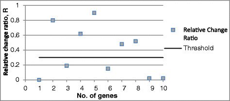
Schematic example for RCR method applied to a gene knockout dataset with an RCR threshold of 0.30.

If the absolute change of gene expression values compared to their own reference value is less than a chosen threshold (e.g., 0.05), even though the relative change ratio is more than 0.30, we still consider these genes as noise and remove them from the regulated genes list.

Dynamic Bayesian network

Dynamic Bayesian network (DBN) analysis is the temporal extension of Bayesian network analysis. It is a general model class that is capable of representing complex temporal stochastic processes. An example of basic DBN block is shown in Figure 2.

Figure 2.

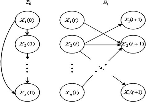
A basic building block of DBN.

A DBN is defined as a pair (B 0, B 1) representing the joint probability distribution over all possible time series of variables X = {X₁, X₂,…X_n}, where X_i(1 ≤ i ≤ n) represents the binary-valued random variables in the network. In addition, the lowercase x_i (1 ≤ i ≤ n) denotes the values of variable X_i. It is composed of initial states of a Bayesian network B₀ = (G₀, Θ₀) and a transition Bayesian network B₁ = (G₁, Θ₁), where B₀ specifies the joint distribution of the variables in X(0) and B₁ represents the transition probabilities Pr{X(t + 1)|X(t)} for all t. In slice 0, the parents of X_i(0) are assumed to be those specified in the prior network B₀, which means Pa(X_i(0)) ⊆ X(0) for all 1 ≤ i ≤ n; in slice t + 1, the parents of X_i(t + 1) are nodes in slices t, Pa(X_i(t + 1)) ⊆ X(t) for all 1 ≤ i ≤ n and t ≥ 0; the connections only exist between consecutive slices. The joint distribution over a finite list of random variables X(0) ∪ X(1) ∪ ⋯ ∪ X(T) can be expressed as [15],[16]

$$\begin{array}{l}Pr\left\{\mathit{x}\left(0\right),\mathit{x}\left(1\right),\dots ,\mathit{x}\left(\mathit{T}\right)\right\}\\ =Pr\left\{\mathit{x}\left(0\right)\right\}{\displaystyle \prod _{\mathit{t}=0}^{\mathit{T}-1}Pr\left\{\mathit{x}\left(\mathit{t}+1\right)|\mathit{x}\left(\mathit{t}\right)\right\}}\\ ={\displaystyle \prod _{\mathit{i}=1}^{\mathit{n}}Pr\left\{{\mathit{x}}_{\mathit{i}}\left(0\right)|\mathrm{pa}\left({\mathit{X}}_{\mathit{i}}\left(0\right)\right)\right\}\times {\displaystyle \prod _{\mathit{t}=0}^{\mathit{T}-1}{\displaystyle \prod _{\mathit{j}=1}^{\mathit{n}}Pr\{{\mathit{x}}_{\mathit{j}}}}}\left({\mathit{X}}_{\mathit{j}}\left(\mathit{t}+1\right)\right)\}\end{array}$$ 2

Kevin Murphy and co-workers [17],[18] implemented a Bayesian network toolbox (BNT), in which the actual structure learning was performed by calling one of the BNT functions learn_struct_dbn_reveal, which used the REVEAL algorithm [4].

Time-delayed dynamic Bayesian network

In the traditional DBN proposed by [17],[18], the effectiveness is not sufficient for two main reasons. The first is the extremely high computational cost. In Murphy's implementation, all the genes in the dataset are considered as parents (regulators) of a given target gene, which makes it impossible to model large-scale gene networks because of exponentially increasing computational time when the algorithm tries to find all of the subsets of parent genes given a target gene. Usually, the number of genes is restricted to less than 30, and more genes will be too much time consuming according to our testing. The second is that biologically relevant transcriptional time lags cannot be determined in Murphy's BNT, which reduces the inference accuracy of gene regulatory networks.

To address the above limitations of traditional DBN, Zou and Conzen [9] introduced a time-delayed dynamic Bayesian network (TDBN)-based analysis method, which can reconstruct GRNs from time series gene expression data. The improved method can dramatically reduce computational time and significantly increased accuracy. According to [9],[10], most transcriptional regulators exhibit either an earlier or simultaneous change in the expression level when compared to their targets. In this way, one can limit the potential parents of each target gene and thus dramatically decrease the computational cost. The other improvement by Zou and Conzen [9] is to perform an estimation of the transcriptional time lag between potential regulators and their target genes. The time difference between the initial expression change of a potential regulator and its target gene represents a biologically relevant time period.

The initial expression change of a potential regulator is expected to allow a more accurate estimation of the transcriptional time lag between potential regulators and their targets, because it takes into account variable expression relationships of different regulator-target pairs. These improvements in [9] are related to transcriptional time-delayed lags between regulators and target genes, so it can also be considered as a time-delayed DBN and directly used to predict networks from time series gene expression data, such as the trajectory time series data in the DREAM3 challenge.

Inferring networks using a method that combines RCR and TDBN

In this combined method, we first used the simple RCR model to find key genes from the given heterozygous knockdown data and null-mutant knockout data. These key genes have a higher potential than other genes to play critical roles in simulated GRNs. After the data was preprocessed, we constructed a gene interaction network that indicated potential regulation among the selected key genes. The TDBN method was then used to infer another GRN from time series trajectory datasets. If gene interactions exist in both networks inferred by RCR and TDBN methods, we choose these interactions as our predicted edges in our final inferred networks. The predicted networks were assessed against the benchmark networks [13],[14].

Results and discussion

Inferred networks as compared with the true networks

In this work, our approach was applied to inferring GRNs in three different ways: For in silico networks with 10 genes, the gene regulatory networks were inferred only by the RCR method from steady state data, in which we used mainly the gene knockout dataset; for networks with 50 genes, the networks inferred using RCR and TDBN separately were combined into the final networks; for networks with 100 genes, we used only TDBN to reconstruct gene networks from time series trajectory gene expression dataset. In doing this, we sought to determine which method had better performance in inferring gene regulatory networks.

Our approach successfully inferred networks using the synthetic datasets provided by Marbach and his colleagues [8],[13],[14]. For example, one of the inferred E. coli 10-node GRN is shown in Figure 3, where seven matching edges are correctly identified by our model, in comparison to the corresponding true network. Our model correctly identified directionality in each of the matching edges. One of the predicted 50-node yeast GRN is shown in Figure 4, and the matching network is shown in Figure 5. There are 52 edges correctly inferred by our method, out of a total of 77 edges in the true network.

Figure 3.

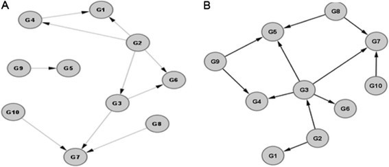
Comparison between a predicted gene regulatory network (A) and the true network (B) for E. coli . Network size = 10 nodes.

Figure 4.

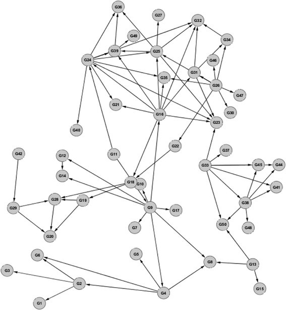
An inferred gene regulatory network for the yeast S. cerevisiae. Network size = 50 nodes.

Figure 5.

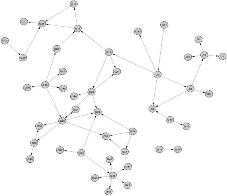
Matching edges between inferred and true networks. The 52 correct edges in the inferred gene regulatory network (shown in Figure 4) that matched with the true network of the yeast S. cerevisiae (network size = 50 nodes).

Performance of network inference from synthetic datasets

The performance of each method was evaluated by two metrics: the area under the precision-recall (AUPR) curve and the area under the receiver operating characteristic (AUROC) curve for the whole set of edge predictions for 15 networks [13],[14]. Precision is a measure of fidelity, whereas recall is a measure of completeness. Recall (R) is defined as $\raisebox{1ex}{$\mathrm{Ce}$}\!\left/ \!\raisebox{-1ex}{$\left(\mathrm{Ce}+\mathrm{Me}\right)$}\right.$ and precision (P) as $\raisebox{1ex}{$\mathrm{Ce}$}\!\left/ \!\raisebox{-1ex}{$\left(\mathrm{Ce}+\mathrm{Fe}\right)$}\right.$, where Ce is the number of correct edges, Me is the total number of missed edges (missed errors), and Fe is the number of false alarm errors. A missed error is defined as the connection between genes that exists in true networks, but the inference algorithms miss or make wrong orientations. A false alarm error is the connection that the inference algorithms create but does not exist in true networks.

A P value is the probability that a given or larger area under the curve value is obtained by random ordering of the T potential network links. An overall P value is the geometric mean of the n individual P values, calculated as ${\left({\mathit{p}}_1\times {\mathit{p}}_2\times \dots \times {\mathit{p}}_{\mathit{n}}\right)}^{1/\mathit{n}}$. An overall AUROC P value represents the geometric mean of the five AUROC P values (Ecoli1, Ecoli2, Yeast1, Yeast2, and Yeast3). An overall AUPR P value is the geometric mean of the five AUPR P values.

To calculate AUPR and AUROC, each predicted network was submitted in the form of ranked lists of predicted edges. The lists were ordered according to the confidence of the predictions so that the first entry corresponded to the edge predicted with the highest confidence. In other words, the edges at the top of the list were believed to be present in the network, and the edges at the bottom of the list were believed to be absent from the network [13].

The inferred GRNs of different sizes (10, 50, and 100 genes) for both E. coli and yeast were evaluated by the above metrics. The larger scores of AUPR and AUROC and the smaller P values of AUPR and AUROC indicate the greater statistical significance of the prediction (Table 1). The metrics of RCR and TDBN inferred networks from the 10- and 50-gene datasets were ranked second among all 29 teams participating in the DREAM3 challenge. The RCR and TDBN inferred networks from the 100-gene dataset were ranked at the 15th place. The overall performance of our methods for all three-sized networks ranked second out of all participating teams in the DREAM3 challenge.

Table 1.

Assessment metrics for the first set of E. coli and yeast networks inferred using our approach

Metrics	Ecoli1_10	Yeast1_10	Ecoli1_50	Yeast1_50	Ecoli1_100	Yeast1_100
AUPR	5.43E − 01	7.71E − 01	6.71E − 01	4.86E − 01	1.45E − 02	1.55E − 02
AUROC	7.94E − 01	9.44E − 01	8.62E − 01	8.35E − 01	5.21E − 01	4.61E − 01
P _AUPR	1.34E − 04	2.09E − 06	8.57E − 55	3.91E − 39	2.27E − 01	8.91E − 01
P _AUROC	5.47E − 04	1.29E − 06	3.19E − 20	4.64E − 18	2.02E − 01	9.60E − 01
Overall AUPR	1.09E − 04		2.54E − 46		4.83E − 03
Overall AUROC	2.10E − 04		8.19E − 18		2.13E − 02

The network name consists of two parts: organism name and network set number (i.e., Ecoli1 or Yeast1) followed by network size (10, 50, or 100 genes). The two parts are separated by ‘_’.

Role of RCR and TDBN in network inference

In general, our predictions of networks with 10 and 50 genes were better than those of 100-gene networks. In most cases, predictions of E. coli networks were better than those of the yeast networks, with the exception of Yeast1 (Table 2). Based on these results, RCR appears to increase the fidelity of network inference more than using TDBN alone. This might explain why the performance of inferred networks with 100 genes was not as good as with size 10 and size 50, because only TDBN was used to infer networks instead of combining prior knowledge which would be gained from preprocessing data by RCR.

Table 2.

Overall performance of our approach for predicting all five sets of networks of different sizes

Size	Metrics	Ecoli1	Ecoli2	Yeast1	Yeast2	Yeast3
10	AUPR	0.544	0.748	0.771	0.352	0.493
	AUROC	0.794	0.856	0.944	0.590	0.715
50	AUPR	0.671	0.672	0.486	0.367	0.381
	AUROC	0.862	0.842	0.836	0.688	0.728
100	AUPR	0.015	0.052	0.016	0.046	0.044
	AUROC	0.521	0.544	0.461	0.576	0.428

The AUPR and AUROC metrics for the first set of networks (Ecoli1 and Yeast1) are reported in Table 1.

To better understand the role of RCR in GRN inference, we used the networks with 10 genes as an example and compared the performance of all three methods: RCR (using only knockout data), TDBN (using time series data without four perturbations), and the combined method (using knockout results as prior knowledge and then running TDBN with time series data). The AUPR, AUROC, and overall score (−0.5 × log₁₀(P _AUPR × P _AUROC)) results obtained for the five datasets in the networks with 10 genes are shown in Figure 6A,B,C, respectively. The three metrics demonstrate that for all five tested datasets, both RCR and the combined method had better performance than TDBN. The combined method was expected to have better performance than the RCR method because the RCR results could provide prior knowledge for TDBN. For three testing datasets (Ecoli2, Yeast1, and Yeast3), the combined method performed better than RCR. But the combined method did not perform as well for the other two datasets (Ecoli1 and Yeast2). Therefore, whether RCR or the combined method has better performance depends on specific datasets. Such an observation can be explained by examining the algorithm in the TDBN method. Even though we specified ‘parent regulators’ as prior knowledge in TDBN to narrow down the search space of regulators, TDBN still calculated its own ‘parents’ based on simultaneously altered time series genes and combined two sets of parents as one group. Thus, TDBN in the combined method always inferred more connections than RCR, which might result in higher false positive rates. How to take advantage of RCR-inferred prior knowledge in the method combining RCR and TDBN to improve the performance of GRN inference remains a challenging research topic that requires further investigations.

Figure 6.

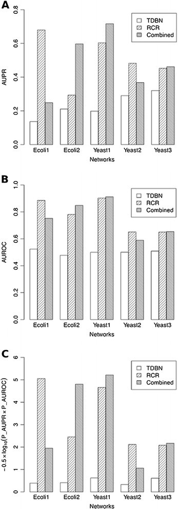
Performance comparison between RCR, TDBN, and combined methods for the 10-node network inference. As evaluated by three metrics. (A) AUPR, (B) AUROC, and (C) an overall score defined as −0.5 × log₁₀(P _AUPR × P _AUROC).

Impact of RCR threshold on network inference accuracy

In the above analyses, we chose an empirical value of 0.30 as the RCR threshold, which implies that a gene is a potential key gene and plays an important role in the network if its change ratio is greater than 0.30. However, it is noteworthy that different RCR thresholds may affect the accuracy of network inference. To investigate the impact of a chosen RCR threshold on the prediction accuracy, we used the networks with 10 genes as an example and calculated both AUPR and AUROC P values, denoted as P-AUPR and P-AUROC, corresponding to 14 different RCR thresholds ranging from 0.05 to 0.70. As shown in Figure 7A,B, both P-AUPR and P-AUROC values were small when a RCR threshold was between 0.15 and 0.40. Furthermore, we also calculated the overall score −0.5 × log₁₀(P _AUPR × P _AUROC) to evaluate the impact of RCR values on the performance. This score was used by the DREAM3 challenges to assess the performance of all participating teams. As shown in Figure 7C, the RCR threshold of 0.25 gave the best performance and it was very close to the empirical RCR threshold we used for GRN inference for the DREAM3 challenges.

Figure 7.

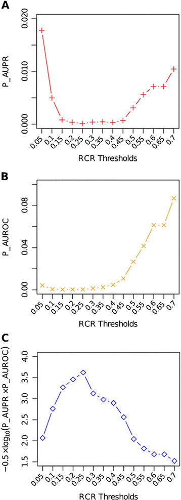
Impact of RCR thresholds on inference performance of the 10-node networks. As evaluated by (A) P _AUPR, (B) P _AUROC, and (C) an overall score defined as −0.5 × log10(P _AUPR × P _AUROC).

Conclusions

In this study, a novel relative change ratio method was proposed to preprocess the null-mutant steady state data in order to find the key genes and build GRNs, in which these selected key genes have a higher potential than other genes to play very critical roles. Then, TDBN was used to infer GRNs from time series trajectory data, which were combined with previous knowledge gained in the initial step. Finally, the inferred networks were evaluated by using AUPR and AUROC metrics for the whole edge predictions for a network. The overall prediction results suggest that our approach was able to infer gene regulatory networks from in silico DREAM challenge data very efficiently and accurately in comparison with other participating teams. We have confidence that the DREAM project will eventually lead the reverse engineering community to resolve technical problems and overcome barriers between research groups towards reliable and accurate GRN inference from high dimensional gene expression data.

Abbreviations

AUPR

area under the precision-recall curve

AUROC

area under the receiver operating characteristic (ROC) curve

DREAM

Dialogue for Reverse Engineering Assessments and Methods

GRN

gene regulatory network

RCR

relative change ratio

TDBN

time-delayed dynamic Bayesian network

Authors’ original submitted files for images

Below are the links to the authors’ original submitted files for images.

Authors’ original file for figure 1 ^{(6.3KB, gif)}

Authors’ original file for figure 2 ^{(29.1KB, gif)}

Authors’ original file for figure 3 ^{(27.4KB, gif)}

Authors’ original file for figure 4 ^{(76.1KB, gif)}

Authors’ original file for figure 5 ^{(62.6KB, gif)}

Authors’ original file for figure 6 ^{(139.4KB, gif)}

Authors’ original file for figure 7 ^{(37.1KB, gif)}

References

- 1.Lähdesmäki H, Shmulevich I, Yli-Harja O. On learning gene regulatory networks under the Boolean network model. Mach. Learn. 2003;52(1–2):147–167. doi: 10.1023/A:1023905711304. [DOI] [Google Scholar]
- 2.Faith JJ, Hayete B, Thaden JT, Mogno I, Wierzbowski J, Cottarel G, Kasif S, Collins JJ, Gardner TS. Large-scale mapping and validation of Escherichia coli transcriptional regulation from a compendium of expression profiles. PLoS Biol. 2007;5(1):e8. doi: 10.1371/journal.pbio.0050008. [DOI] [PMC free article] [PubMed] [Google Scholar]
- 3.Chen I, He HL, Church GM. Modeling gene expression with differential equations. Pac. Symp. Biocomput. 1999;4:29–40. [PubMed] [Google Scholar]
- 4.Liang S, Fuhrman S, Somogyi R. REVEAL, a general reverse engineering algorithm for inference of genetic network architectures. Pac. Symp. Biocomput. 1998;3:18–29. [PubMed] [Google Scholar]
- 5.Imoto S, Goto T, Miyano S. Estimation of genetic networks and functional structures between genes by using Bayesian networks and nonparametric regression. Pac. Symp. Biocomput. 2002;7:175–186. [PubMed] [Google Scholar]
- 6.Stolovitzky G, Prill RJ, Califano A. Lessons from the DREAM2 challenges. Ann. N Y Acad. Sci. 2009;1158(1):159–195. doi: 10.1111/j.1749-6632.2009.04497.x. [DOI] [PubMed] [Google Scholar]
- 7.Mendes P, Sha W, Ye K. Artificial gene networks for objective comparison of analysis algorithms. Bioinformatics. 2003;19(2):122–129. doi: 10.1093/bioinformatics/btg1069. [DOI] [PubMed] [Google Scholar]
- 8.Marbach D, Schaffter T, Mattiussi C, Floreano D. Generating realistic in silico gene networks for performance assessment of reverse engineering methods. J. Comput. Biol. 2009;16(2):229–239. doi: 10.1089/cmb.2008.09TT. [DOI] [PubMed] [Google Scholar]
- 9.Zou M, Conzen SD. A new dynamic Bayesian network (DBN) approach for identifying gene regulatory networks from time course microarray data. Bioinformatics. 2005;21(1):71–79. doi: 10.1093/bioinformatics/bth463. [DOI] [PubMed] [Google Scholar]
- 10.Yu H, Luscombe NM, Qian J, Gerstein M. Genomic analysis of gene expression relationships in transcriptional regulatory networks. Trends Genet. 2003;19:422–427. doi: 10.1016/S0168-9525(03)00175-6. [DOI] [PubMed] [Google Scholar]
- 11.Stolovitzky G, Monroe D, Califano A. Dialogue on reverse-engineering assessment and methods: the dream of high-throughput pathway inference. Ann. N Y Acad. Sci. 2007;1115:1–22. doi: 10.1196/annals.1407.021. [DOI] [PubMed] [Google Scholar]
- 12.Cantone I, Marucci L, Iorio F, Ricci MA, Belcastro V, Bansal M, Santini S, Bernardo MD, Bernardo DD, Cosma MP. A yeast synthetic network for in vivo assessment of reverse-engineering and modeling approaches. Cell. 2009;137:172–181. doi: 10.1016/j.cell.2009.01.055. [DOI] [PubMed] [Google Scholar]
- 13.Marbach D, Prill RJ, Schaffter T, Mattiussi C, Floreano D, Stolovitzky G. Revealing strengths and weaknesses of methods for gene network inference. Proc. Natl. Acad. Sci. U S A. 2010;107(14):6286–6291. doi: 10.1073/pnas.0913357107. [DOI] [PMC free article] [PubMed] [Google Scholar]
- 14.Prill RJ, Marbach D, Saez-Rodriguez J, Sorger PK, Alexopoulos LG, Xue X, Clarke ND, Altan-Bonnet G, Stolovitzky G. Towards a rigorous assessment of systems biology models: the DREAM3 challenges. PLoS One. 2010;5(2):e9202. doi: 10.1371/journal.pone.0009202. [DOI] [PMC free article] [PubMed] [Google Scholar]
- 15.Lähdesmäki H, Hautaniemi S, Shmulevich I, Yli-Harja O. Relationships between probabilistic Boolean networks and dynamic Bayesian networks as models of gene regulatory networks. Signal Process. 2006;86(4):814–834. doi: 10.1016/j.sigpro.2005.06.008. [DOI] [PMC free article] [PubMed] [Google Scholar]
- 16.Friedman N, Murphy K, Russell S. Proceedings of the Fourteenth Conference on Uncertainty in Artificial Intelligence (UAI) 1998. Learning the structure of dynamic probabilistic networks; pp. 139–147. [Google Scholar]
- 17.Murphy K. Dynamic Bayesian networks: representation, inference and learning. Berkeley: University of California; 2002. [Google Scholar]
- 18.Murphy K, Mian S. Modeling gene expression data using dynamic Bayesian networks. Berkeley, CA: University of California; 1999. [Google Scholar]