Understanding the Impact of Stroke on Brain Motor Function: A Hierarchical Bayesian Approach

Abstract

Stroke is a disturbance in blood supply to the brain resulting in the loss of brain functions, particularly motor function. A study was conducted by the UCI Neurorehabilitation Lab to investigate the impact of stroke on motor-related brain regions. Functional MRI (fMRI) data were collected from stroke patients and healthy controls while the subjects performed a simple motor task. In addition to affecting local neuronal activation strength, stroke might also alter communications (i.e., connectivity) between brain regions. We develop a hierarchical Bayesian modeling approach for the analysis of multi-subject fMRI data that allows us to explore brain changes due to stroke. Our approach simultaneously estimates activation and condition-specific connectivity at the group level, and provides estimates for region/subject-specific hemodynamic response functions. Moreover, our model uses spike and slab priors to allow for direct posterior inference on the connectivity network. Our results indicate that motor-control regions show greater activation in the unaffected hemisphere and the midline surface in stroke patients than those same regions in healthy controls during the simple motor task. We also note increased connectivity within secondary motor regions in stroke subjects. These findings provide insight into altered neural correlates of movement in subjects who suffered a stroke.

1. INTRODUCTION

Stroke is a disturbance in the blood supply to the brain that results in the death of neural tissue and subsequent behavioral deficits arising from the affected brain systems. One of the most commonly affected neural systems is the motor system, causing disability in people who suffered a stroke. In order to compensate for the loss of brain function in the affected brain area, other areas within the motor system are often recruited—and, therefore, activated—to assist in the execution of movements in stroke-impaired subjects. Also, communications—termed as connectivity in the neuroscience literature—may be altered between regions within the motor network.

To better understand the impact of stroke in brain motor activation and connectivity, we developed a model for analyzing functional magnetic resonance imaging (fMRI) data from a multi-subject stroke study conducted at the University of California Irvine Neurorehabilitation Lab (PI: Cramer). The study recruited healthy subjects and stroke patients with residual motor deficit as it was focused on understanding how brain motor function is altered after stroke. Motor-task-related fMRI scans were acquired for all the participants.

As an imaging modality, fMRI is able to indirectly measure neuronal activity in the brain through the hemodynamic response: higher level of neuronal activity at a localized region requires a greater amount of oxygen, which results in higher level of the blood-oxygen-level-dependent (BOLD) contrast fMRI signal at that location. By analyzing fMRI data, one can study local neuronal activation as well as inter-regional connectivity. The hemodynamic response function (HRF) describes the shape of the hemodynamic response evoked by a point stimulus. The HRF is likely to vary across brain regions and subjects. Thus, it is very important to correctly estimate the HRF for each region and subject in order to correctly infer information regarding activation and connectivity, because neural activity is indirectly measured through the hemodynamic response. The goal of this Bayesian hierarchical modeling approach is to investigate the impact of stroke by comparing brain activation and connectivity of motor-related brain areas between stroke patients and healthy controls, while taking HRF variation into account.

1.1 Overview of the fMRI Stroke Study

The fMRI study involved patients who had suffered a stroke and had residual motor deficit on the right side of the body, and healthy subjects. During the fMRI experiment, each subject alternated between a right hand grasp-release movement (task condition, also called the stimulus condition) and rest (rest condition). Five brain regions of interest (ROI) known to be implicated in motor function are considered for this study (see Figure 1(a)): two primary motor regions including the left and right primary motor cortex (LM1 and RM1), three secondary motor regions including the left and right dorsal premotor cortex (LPMd and RPMd), and a midline supplementary motor area (SMA). Note that a stroke patient with injury on the left brain hemisphere will have motor function deficits on the right side of the body; and vice versa. Typically, when a healthy subject performs a simple right-hand movement task, it is expected that only LM1 (M1 in the left hemisphere) is likely to be activated. RM1 is expected to not activate, since it is primarily responsible for motor function of the left side of the body. The secondary motor regions (SMA and the two PMd regions) are primarily responsible for more advanced motor functions such as motor planning and bilateral coordination.

Figure 1.

(a) Locations of the five regions of interest: LM1 and RM1 (left and right primary motor cortex), LPMd and RPMd (left and right dorsal premotor cortex), and SMA (supplementary motor area). (b) FMRI time series from a healthy subject at LM1 (top) and RM1 (bottom); the lines at the bottom of each plot indicate the task condition (high value) and the rest condition (low value). The time series of the two independent sessions (each with 48 scans) are concatenated on the plot. The dashed lines separate the two sessions.

1.2 Proposed Approach

To analyze these multi-subject fMRI stroke data, we developed a Bayesian approach that jointly estimates activation and connectivity. Our approach provides estimates of subject and region-specific hemodynamic response functions (HRFs). It utilizes the general linear model (GLM) to describe activation, a Bayesian vector-autoregressive model (BVAR) to measure connectivity, and a constrained linear basis set to model the unknown HRFs. The proposed model provides a hierarchical framework that handles group-level activation and connectivity, as well as their variability among subjects. With the hierarchical structure, subject-specific estimates for activation and connectivity are obtained by pooling information from other subjects. Spike and slab priors are placed on the model parameters that describe the connectivity network. This allows us to explore the full posterior distribution of possible connectivity networks. Additionally, we allow condition-specific connectivity measures, thus making it possible to detect differences in connectivity between experimental conditions. Our goal is to study local activation and connectivity between brain regions, and compare the inferred patterns for stroke patients and healthy controls in order to explore the effects of stroke on brain motor function, while controlling for variation in the HRFs.

1.3 Current Statistical Methods and Their Limitations

In the past 20 years, there has been an increasing number of papers on statistical methods for fMRI data. Lindquist (2008) and Zhang et al. (2015) provide detailed reviews on existing methods. Methods for brain activation are proposed in Friston et al. (1994); Worsley and Friston (1995); Smith and Fahrmeir (2007); David et al. (2008); Guo and Pagnoni (2008); Xu et al. (2009); Degras and Lindquist (2014). Methods for brain connectivity are developed in Friston et al. (2003); Harrison et al. (2003); Bowman et al. (2008); Cribben et al. (2012); Kang et al. (2012); Gorrostieta et al. (2013); Luo (2014).

While methods for activation usually do not consider connectivity estimation, David et al. (2008) in fact considered connectivity estimation, but used a two-stage approach that estimates connectivity from the residuals of the activation analysis, and hence is not optimal for properly assessing the uncertainty associated to those estimates. Harrison et al. (2003) estimated connectivity using vector-autoregressive (VAR) models, while Cribben et al. (2012) developed dynamic connectivity regression which models changes in connectivity, but none of these approaches take into account the systematic changes in the BOLD response induced by external stimuli. Gorrostieta et al. (2013) considered the BOLD response evoked by stimuli and also the differential connectivity across different experimental conditions. However, the BOLD response shape was based on a fixed HRF shape for all brain regions and subjects, which may lead to erroneous conclusions when inferring activation and connectivity (Yu et al., 2015). Bowman et al. (2008) and Luo (2014) also took the experimental conditions into account, but modeled connectivity through a two-stage approach and used a pre-specified HRF. Kang et al. (2012) simultaneously analyzed activation and connectivity in the spectral domain, but also used a pre-specified HRF. Friston et al. (2003) used dynamic causal modeling (DCM) which addresses ROI-specific HRF and connectivity simultaneously. However, DCM heavily relies on the correct specification of the biological assumptions, and needs a set of plausible connectivity networks a priori which are difficult to verify from the observed data.

There are many ways to parameterize HRFs. Non-linear parameterization approaches include gamma functions, cosine functions (Zarahn, 2002), or inverse logit functions (Lindquist et al., 2008). Linear basis approaches such as spline basis functions, finite impulse response bases (Ollinger et al., 2001) and semi-parametric models (Zhang et al., 2001) are also available. Non-linear parameterization takes more computational effort and is more prone to the local maxima problem and numerical stability issues. On the other hand, linear parameterization is easier from the inferential viewpoint, but often requires more parameters and constraints in order to provide enough flexibility in modeling HRF shapes. Woolrich et al. (2004) proposed constrained linear basis sets which are able to provide both flexible and reasonable HRF shapes with a relatively small number of HRF basis functions while keeping the computation cost low. Therefore, in this paper we adopt the constrained linear basis approach to parameterize the HRFs.

In a nutshell, we propose a model that has the following advantages over currently available methods: (1) it simultaneously estimates activation, connectivity and HRFs; (2) it provides ROI and subject-specific HRFs, as well as condition-specific connectivity measures; (3) it increases the power in detecting group differences by pooling information across subjects via hierarchical modeling; (4) it provides full posterior distributions of all the model parameters, including group-specific activation parameters and brain connectivity networks; (5) it can incorporate available scientifically relevant prior information. The remainder of the paper is organized as follows. In Section 2 we describe the stroke study and the fMRI data. In Section 3 we develop our approach including the model, the prior distributions and the inferential procedure. In Section 4 we present the simulation studies, and in Section 5 we present the analysis of the fMRI data from the stroke study. We summarize our approach and discuss future research directions in Section 6.

2. EXPERIMENTAL DESIGN AND FMRI DATA

Experiment

The study included 15 stroke patients and 12 healthy control subjects. All the subjects were right-handed. The stroke patients had ischemic stroke on the left brain hemisphere 11 – 26 weeks prior to the study assessments, and continued to have residual motor deficit on the right side of the body at the time of the experiment. During the task condition, the subjects used their right hand to perform the hand grasp-release movement task. For the stroke patients, the right hand was also the hand that was affected by stroke. The experiment was divided into three sessions for stroke patients and two sessions for healthy controls. Each session had 48 consecutive scans, alternating between task and rest conditions twice, but always starting with rest condition (see Figure 2).

Figure 2.

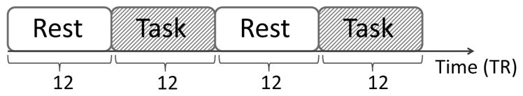
Block design of the experiment for each session.

FMRI data

The fMRI images were acquired using a T2*-weighted gradient-echo-planar imaging sequence with repetition time (TR) = 2 s. Functional data from all the sessions were preprocessed using the SPM8 software (Wellcome Trust Center for Neuroimaging, UCL, 2009). Preprocessing steps included realignment to the first image, coregistration to the mean image, normalization to the standard MNI EPI template, and spatial smoothing (FWHM = 8 mm). The time series for each ROI were obtained by averaging the fMRI signals recorded across the voxels in the region. The mean time series were centered to zero and detrended with time as the covariate to remove the drift effect. Finally, the centered and detrended time series were scaled to have the same variance for all subjects and ROIs within each group.

Selected time series from the LM1 and RM1 regions in a healthy subject are shown in Figure 1(b). The block-shaped line at the bottom indicates the times when the subject performed the motor task. In LM1 (top plot) the fMRI signal generally follows the block-shaped wave with some lag. It rises soon after the task condition begins and drops soon after the task condition ends, which suggests that this region is implicated in the motor task. However, in RM1 (bottom plot) the time series does not appear to be obviously associated with the timing of the motor task.

3. METHODOLOGY

In this section we develop the Bayesian hierarchical modeling approach and related inferential procedures for investigating the effect of stroke on brain motor function, specifically on activation and connectivity of the five ROIs related to motor function. The proposed model will be utilized to infer activation and connectivity at the group level while taking into account subject/region-specific variability in the HRFs.

3.1 Hierarchical Model: Subject Level

To describe the fMRI signal for a given ROI and subject, we use the general linear model:

$$\begin{array}{lll}\hfill y_p^{(s,r)}(t)& =\hfill & {\beta }_{p0}^{(s)}+x_{p1}^{(s,r)}(t){\beta }_{p1}^{(s)}+x_{p2}^{(s,r)}(t){\beta }_{p2}^{(s)}+u_p^{(s,r)}(t),\hfill \\ \hfill x_{pk}^{(s)}(t)& =\hfill & [h_p^{(s)}\ast c_k](t),\hfill \end{array}$$ (1)

with ROI p = 1, 2, …, P ; subject s = 1, 2, …, S; session r = 1, 2, …, R; and time (in a session) t = 1, 2, …, T (TR). The response variable $y_p^{(s,r)}(t)$ is the preprocessed fMRI signal; the covariate $x_{pk}^{(s,r)}(t)$ represents the expected shape of BOLD response, which is the convolution between the HRF, denoted as $h_p^{(s)}(t)$, and the known binary condition indicator with c_k(t), with c_k(t) = 1 when the kth condition is on and zero otherwise (we use k = 1 for the task condition and k = 2 for the rest condition, see Figure 2 for the timing of the conditions); the regression coefficient ${\beta }_{pk}^{(s)}$ represents the amplitude of the BOLD response which indirectly reflects the strength of neuronal activity; and $u_p^{(s,r)}(t)$ is the noise that is not explained by the mean structure. The effect of the convolution is illustrated in Figure 3. The expected BOLD response is no longer block-shaped as the stimulus input, but is a smooth and delayed transformation of the input. In this model, we have imposed the following assumptions: (1) the BOLD amplitude remains the same within a condition and across sessions; (2) the HRF shape within each ROI and subject remains constant across conditions and sessions.

Figure 3.

(a) Canonical HRF. (b) Condition indicator function. (c) BOLD response.

On modeling activation

Neuroscientists are interested in estimating the difference between activity strength of two conditions as measured by a region-specific contrast, i.e., ${\beta }_{p,(c)}^{(s)}={\beta }_{p1}^{(s)}-{\beta }_{p2}^{(s)}$. When ROI p shows stronger activity during the task than during the control condition, it suggests that this ROI is implicated in executing the task. Therefore, when ${\beta }_{p,(c)}^{(s)}>0$, ROI p is labeled as active in subject s, and ${\beta }_{p,(c)}^{(s)}$is used to measure the strength of the local activation.

On modeling connectivity

Following Gorrostieta et al. (2013), the noise u^(s,r)(t) ∈ ℝ^P is assumed to follow a Gaussian vector autoregressive model (VAR) with pre-determined order L and condition-dependent VAR coefficients, i.e.,

$${\mathit{u}}^{(s,r)}(t)={[u_1^{(s,r)}(t),\dots ,u_P^{(s,r)}(t)]}^{\prime }=\sum _{\ell =1}^L{\mathrm{\Phi }}^{\ast (s)}(\ell ,t){\mathit{u}}^{(s,r)}(t-\ell )+{\mathit{\epsilon }}^{(s,r)}(t),$$

where ${\mathit{\epsilon }}^{(s)}(t)={[{\epsilon }_1^{(s,r)}(t),\dots ,{\epsilon }_P^{(s,r)}(t)]}^{\prime }\stackrel{\mathit{ind}}{\sim }N(\mathbf{0},{\mathrm{\sum }}^{(s)})$, and

$${\mathrm{\Phi }}^{\ast (s)}(\ell ,t)=c_1(t-\ell ){\mathrm{\Phi }}_1^{\ast (s)}(\ell )+c_2(t-\ell ){\mathrm{\Phi }}_2^{\ast (s)}(\ell ).$$ (2)

Denote the (p, q)-th element of Φ^*(s)(ℓ, t) as Φ^*(s)(ℓ, t)_pq. This quantity describes the linear relation between ROIs p and q at time lag ℓ: when Φ^*(s)(ℓ, t)_pq ≠ 0, ROI q at time t − ℓ helps predict ROI p at the current time point t. The temporal precedence of ROI q in this relationship suggests the interpretation of Φ^*(s)(ℓ, t)_pq as a measure of the directed influence from ROI q to ROI p. This type of influence is termed as “effective connectivity” in neuroscience. Therefore, Φ^*(s)(ℓ, t)_pq can be used to measure effective connectivity from ROI q to ROI p. For simplicity, in the remainder of this paper we refer to this as “connectivity”. Also, it is possible that the manner in which an ROI influences another varies under different conditions. Hereby, we allow Φ^*(s)(ℓ, t)_pq to depend on the condition at the corresponding past time point as specified in Equation (2).

We use a Bayesian variable selection approach (Mitchell and Beauchamp, 1988; George and McCulloch, 1993; Ishwaran and Rao, 2005) to determine which elements of Φ^*(s)(ℓ, t) are different from zero, and therefore infer the connectivity network across ROIs. More specifically, we impose a “spike and slab” structure on ${\mathrm{\Phi }}_k^{\ast (s)}$ given by

$${\mathrm{\Phi }}_k^{\ast (s)}{(\ell )}_{pq}={\mathrm{\Phi }}_k^{(s)}{(\ell )}_{pq}{\mathit{\xi }}_{pq}^{(s)}(\ell ),\text{with}{\mathrm{\Phi }}_k^{(s)}{(\ell )}_{pq}\in ℝ,{\mathit{\xi }}_{pq}^{(s)}(\ell )\in \{0,1\},$$ (3)

so that ${\mathrm{\Phi }}_k^{\ast (s)}{(\ell )}_{pq}=0\iff {\mathit{\xi }}_{pq}^{(s)}(\ell )=0(\text{a.s.});Pr({\mathrm{\Phi }}_k^{\ast (s)}{(\ell )}_{pq}\ne 0)=Pr({\mathit{\xi }}_{pq}^{(s)}(\ell )=1)$, and ${\mathrm{\Phi }}_k^{\ast (s)}{(\ell )}_{pq}={\mathrm{\Phi }}_k^{\ast (s)}{(\ell )}_{pq}\iff {\mathit{\xi }}_{pq}^{(s)}(\ell )=1(\text{a.s.})$. When ${\mathrm{\Phi }}_k^{\ast (s)}{(\ell )}_{pq}=0$, or equivalently when ${\mathit{\xi }}_{pq}^{(s)}(\ell )=0$ for all ℓ, we say that there is no connectivity from ROI q to ROI p. Otherwise, there is connectivity from ROI q to ROI p.

On HRF modeling

A linear basis for the representation of the HRFs was obtained based on the approach of Woolrich et al. (2004). In particular, using this approach, the HRF of subject s and region p can be written in terms of J basis vectors as $h_p^{(s)}(t)={\sum }_{j=1}^{J}H(t,j)d_{pj}^{(s)}$, where H is the T × J basis matrix with each column being a basis vector, and ${\mathit{d}}_p^{(s)}\in {ℝ}^J$ is the vector of HRF basis coefficients for ROI p and subject s. For identifiability, we impose a normalization constraint on ${\mathit{d}}_p^{(s)}$ so that ${\sum }_{t=1}^T{h}_p^{(s)}(t)=1$. Further details on the basis representation and how to choose J are given in Section 3.3.

We use A(i, :), A(:, j), and A(i, j) to denote, respectively, the i-th row, the j-th column, and the (i, j)-th element of any matrix A. Then, $h_p^{(s)}(t)$ can be written as $H(t,:){\mathit{d}}_p^{(s)}$ with ${\mathit{d}}_p^{(s)}\in {ℝ}^J=[d_{p1}^{(s)},\dots ,d_{pJ}^{(s)}]$, and $x_{pk}^{(s)}(t)$ can be written as $x_{pk}^{(s)}(t)=[H\ast c_k](t,:){\mathit{d}}_p^{(s)}:={\mathrm{\Lambda }}_k(t,:){\mathit{d}}_p^{(s)}$, t = 1, 2, …, T, where the matrix Λ_k ∈ ℝ^T×J consists of the convolutions between each linear basis vector H(:, j), and the condition indicator c_k(t). Therefore, combining this with Equation (1) leads to

$$y_p^{(s,r)}(t)={\beta }_{p0}^{(s)}+{\mathrm{\Lambda }}_1(t,:){\mathit{d}}_p^{(s)}{\beta }_{p1}^{(s)}+{\mathrm{\Lambda }}_2(t,:){\mathit{d}}_p^{(s)}{\beta }_{p2}^{(s)}+u_p^{(s,r)}(t).$$

3.2 Hierarchical Model: Group Level

Since the signal to noise ratio is usually low in fMRI data (typically below 5%), it is beneficial to borrow information across subjects within a relatively homogeneous group. In order to do this, we use a Bayesian hierarchical modeling approach. We define ${\mathit{\beta }}_p^{(s)}={[{\beta }_{p0}^{(s)},{\beta }_{p1}^{(s)},{\beta }_{p2}^{(s)}]}^{\prime },{\mathit{\beta }}^{(s)}={[{({\mathit{\beta }}_1^{(s)})}^{\prime },\dots ,{({\mathit{\beta }}_P^{(s)})}^{\prime }]}^{\prime };{\mathit{\varphi }}_k^{(s)}=[\text{vec}{({\mathrm{\Phi }}_k^{(s)}(1))}^{\prime },\dots ,\text{vec}{({\mathrm{\Phi }}_k^{(s)}(L))}^{\prime }],{\mathit{\varphi }}^{(s)}={[{({\mathit{\varphi }}_1^{(s)})}^{\prime },{({\mathit{\varphi }}_2^{(s)})}^{\prime }]}^{\prime },{\mathit{\xi }}_{pq}^{(s)}=[{\mathit{\xi }}_{pq}^{(s)}(1),\dots ,{\mathit{\xi }}_{pq}^{(s)}(L)]$ and ${\mathit{d}}^{(s)}={[{({\mathit{d}}_1^{(s)})}^{\prime },\dots ,{({\mathit{d}}_P^{(s)})}^{\prime }]}^{\prime }$. We then assume that each of the S subjects belongs to a single group, denoted by g_s, from a total of G groups (e.g., in our case we have stroke patients and healthy controls, so G = 2), and consider the following distributions,

$$\begin{array}{lll}{\mathit{\beta }}^{(s)}\hfill & \stackrel{\mathit{ind}}{\sim }\hfill & N({\mathit{\mu }}_{\mathit{\beta }}^{g_s},{\mathrm{\sum }}_{\mathit{\beta }}^{g_s}),{\mathit{d}}^{(s)}\stackrel{\mathit{ind}}{\sim }N({\mathit{\mu }}_{\mathit{d}}^{g_s},{\mathrm{\sum }}_{\mathit{d}}^{g_s}),{\mathit{\varphi }}^{(s)}\stackrel{\mathit{ind}}{\sim }N({\mathit{\mu }}_{\mathit{\varphi }}^{g_s},{\mathrm{\sum }}_{\mathit{\varphi }}^{g_s}),\hfill \\ {\mathit{\xi }}_{pq}^{(s)}\hfill & \stackrel{\mathit{ind}}{\sim }\hfill & \mathit{Multinomial}(1,{\mathit{\pi }}_{pq}^{g_s}),{\mathrm{\sum }}^{(s)}\stackrel{\mathit{ind}}{\sim }\mathit{InvWishart}({\mathrm{\sum }}^{g_s},{\nu }_{\mathrm{\sum }}).\hfill \end{array}$$

Here $Pr({\mathit{\xi }}_{pq}^{(s)}={\mathit{\ell }}_j)={\mathit{\pi }}_{pq}^{g_s}(j)$, where ${\mathit{\ell }}_j=[\underset{j1’\mathrm{s}}{\underbrace{1,\dots ,1}},\underset{L-j0’\mathrm{s}}{\underbrace{0,\mathrm{..},0}}]$, j = 0, 1, …, L. The j in ${\mathit{\xi }}_{pq}^{(s)}={\mathit{\ell }}_j$ can be interpreted as the largest lag at which there is connectivity from ROI q to ROI p.

Therefore, all the subjects belonging to the same group, say group g, will have the same group parameters ${\mathit{\mu }}_{\mathit{\beta }}^g,{\mathrm{\sum }}_{\mathit{\beta }}^g,{\mathit{\mu }}_{\mathit{d}}^g,{\mathrm{\sum }}_{\mathit{d}}^g,{\mathit{\mu }}_{\mathit{\varphi }}^g,{\mathrm{\sum }}_{\mathit{\varphi }}^g,{\mathit{\pi }}_{pq}^g$, and Σ^g. Note that ${\mathit{\mu }}_{\mathit{\beta }}^g$ are the mean BOLD amplitudes and intercepts for group g, ${\mathit{\mu }}_{\mathit{d}}^g$ are the mean HRF basis coefficients, ${\mathit{\mu }}_{\mathit{\varphi }}^g$ are the mean connectivity strengths, and ${\mathit{\pi }}_{pq}^g(\ell )$ is the overall probability that connectivity from ROI q to ROI p exists up to ℓ lags among the group. For simplicity, ν_Σ is taken as a fixed constant across groups, and ${\mathrm{\sum }}_{\mathit{\beta }}^{g_s},{\mathrm{\sum }}_{\mathit{d}}^{g_s}$ and ${\mathrm{\sum }}_{\mathit{\varphi }}^{g_s}$ are assumed to be diagonal.

For any g, the distributions for the group parameters are taken as ${\mathit{\mu }}_{\mathit{\beta }}^g\stackrel{\mathit{ind}}{\sim }N({\mathit{\mu }}_{{\mathit{\mu }}_{\mathit{\beta }},0},{\mathrm{\sum }}_{{\mathit{\mu }}_{\mathit{\beta }},0}),{\mathrm{\sum }}_{\mathit{\beta }}^g(i,i)\stackrel{\mathit{ind}}{\sim }\mathit{InvGamma}(a_{\mathit{\beta }},b_{\mathit{\beta }}),{\mathit{\mu }}_{\mathit{d}}^g\stackrel{\mathit{ind}}{\sim }N({\mathit{\mu }}_{{\mathit{\mu }}_{\mathit{d}},0},{\mathrm{\sum }}_{{\mathit{\mu }}_{\mathit{d}},0}),{\mathrm{\sum }}_{\mathit{d}}^g(i,i)\stackrel{\mathit{ind}}{\sim }\mathit{InvGamma}(a_{\mathit{d}},b_{\mathit{d}}),{\mathit{\mu }}_{\mathit{\varphi }}^g\stackrel{\mathit{ind}}{\sim }N({\mathit{\mu }}_{{\mathit{\mu }}_{\mathit{\varphi }},0},{\mathrm{\sum }}_{{\mathit{\mu }}_{\mathit{\varphi }},0}),{\mathrm{\sum }}_{\mathit{\varphi }}^g(i,i)\stackrel{\mathit{ind}}{\sim }\mathit{InvGamma}(a_{\mathit{\varphi }},b_{\mathit{\varphi }}),{\mathit{\pi }}_{pq}^g\stackrel{\mathit{ind}}{\sim }\mathit{Dir}({\mathit{\alpha }}_{\mathit{\pi }})$, and $p({\mathrm{\sum }}^g)\propto {\mid {\mathrm{\sum }}^g\mid }^{-\frac{1+P}{2}}$. Here μ_μβ,0, Σ_μβ,0, μ_μϕ,0, Σ_μϕ,0, a_β, b_β, a_d, b_d, a_ϕ, b_ϕ, and α_π are pre-determined constants. The choices of these constants will be discussed in Sections 4 and 5. In fMRI datasets with more than two groups, another level can be added to the hierarchy by imposing additional priors on the group parameters for activation, connectivity and those related to the HRFs.

The Bayesian hierarchical model is now fully specified. The quantities of interest are as follows.

Activation for ROI p

${\beta }_{p1}^{(s)}-{\beta }_{p2}^{(s)}$ is the activation strength for subject s, and ${\mu }_{\beta ,p1}^g-{\mu }_{\beta ,p2}^g$ is the mean activation strength for group g (group-level activation strength). Here ${\mu }_{\beta ,pk}^g$ denotes the element in ${\mathit{\mu }}_{\mathit{\beta }}^g$ corresponding to ${\mathit{\beta }}_{pk}^{(s)}$.

Connectivity from ROI q to ROI p

$Pr({\mathit{\xi }}_{pq}^{(s)}(\ell )=1)$ is the probability that such connectivity is present at lag ℓ for subject s, for ℓ = 1, …, L; ${\mathrm{\Phi }}_k^{\ast (s)}{(\ell )}_{pq}$, is the measure of the connectivity strength under condition k at lag ℓ for subject s; ${\mathit{\pi }}_{pq}^g(\ell )$ is the probability that the largest lag of such connectivity is ℓ for group g (group-level presence probability of connectivity), and ${\mu }_{{\mathrm{\Phi }}_k(\ell ),pq}^g$ is the mean connectivity for the group, (group-level connectivity strength).

HRF for ROI p

${\mathit{h}}_p^{(s)}=H{\mathit{d}}_p^{(s)}$ is the HRF of ROI p for subject s and ${\mathit{\mu }}_{h_p}^g=H{\mathit{\mu }}_{{\mathit{d}}_p}^g$ is the mean HRF of ROI p for group g.

In the particular case of the stroke study, based on a preliminary analysis of the data, we found that there is a large within-group variability in the shape of the HRFs across subjects (see Figure 4). The preliminary analysis was done by computing the posterior mode of the activation and HRF parameters using a conditional maximization algorithm, ignoring all the dependence across time, ROIs and subjects. We note that averaging curves of very different shapes within a group is likely to produce meaningless overall group-specific shapes due to the non-linearity involved. Hence, it is prudent to not pool the highly heterogeneous shapes of the HRFs across subjects. Therefore, specifically for the analysis of the stroke data, we fix ${\mathit{\mu }}_{\mathit{d}}^g$ as a constant. This will be discussed in detail in the next subsection. However, we still combine information on activation and connectivity from other subjects.

Figure 4.

A preliminary analysis of HRFs. (a) HRFs of all healthy subjects at a given ROI. (b) HRFs of all stroke subjects at the same ROI. The black curve is canonical HRF.

3.3 Constrained Linear Basis for the HRFs

Here we briefly describe how to obtain the constrained linear basis for the HRFs. Following the general framework of Woolrich et al. (2004), one can simulate n discrete HRF vectors based on the half-cosine parameterization. The parameters involved are the temporal resolution δ, the duration parameters h₁, h₂, h₃, h₄, and the depth parameters f₁ and f₂ (see Figures A.1(a) and A.1(b) in the Appendix). Using principal component analysis (PCA) one can obtain J linear basis vectors for the HRFs, and the corresponding basis coefficients (loadings of the top J components), denoted as d_i, for the i-th simulated HRF, i = 1, 2, …, n. For the simulation study and the fMRI data analysis in this paper we used n = 1000, δ = 0.1, h₁ ~ Unif(0, 2), h₂ ~ Unif(2, 7), h₃ ~ Unif(2, 8), h₄ ~ Unif(2, 12), f₁ = 0, f₂ ~ Unif(0, 0.5), and J = 5. The reason for choosing J = 5 is that the top 5 principal components for the HRF basis set, i.e., the first J = 5 columns of the matrix H, explain about 99% of the total variability in the simulated HRFs (see Figure A.2(a) in the Appendix). Note that it is also the case that the first HRF basis vector is very similar to the canonical HRF (see Figure A.2(b) in the Appendix).

As a next step, we compute the empirical mean ${\mathit{\mu }}_{\mathit{d}}^{\ast }\in {ℝ}^J$ and variance ${\mathrm{\sum }}_{\mathit{d}}^{\ast }\in {ℝ}^{J\times J}$ of the basis coefficients ${\{{\mathit{d}}_i\}}_{i=1}^n$. We then use the Gaussian distribution, $N({\mathit{\mu }}_{\mathit{d}}^{\ast },{\mathrm{\sum }}_{\mathit{d}}^{\ast })$, as the prior distribution for the HRF basis coefficients d^(s), i.e., use ${\mathit{\mu }}_{\mathit{d}}^g={\mathit{\mu }}_{\mathit{d}}^{\ast }$ and ${\mathrm{\sum }}_{\mathit{d}}^g={\mathrm{\sum }}_{\mathit{d}}^{\ast }$ for all g. Such prior distribution on the constrained linear basis representation provides enough flexibility to capture the HRF shapes, e.g., time to peak, width of peak and time to undershoot, and simultaneously penalizes shapes that deviate from the space of reasonable shapes. Note that our prior beliefs about the HRFs are adopted through the choice of the duration parameters and the depth parameters. The normal distribution just provides a convenient approximation of such prior beliefs. In order to determine if the prior structure is reasonable, visual checks of the quality of the basis set can be performed by generating prior samples of the HRFs using the basis vectors and corresponding coefficients randomly sampled from the normal distribution described above. Figure A.2(c) displays examples of randomly generated HRFs from the HRF basis set used in our analysis. The HRFs sampled from the prior indicate that this HRF basis representation is sufficiently flexible in capturing time to peak, width of peak, time to undershoot, and lead to reasonable HRF shapes.

3.4 Posterior Inference via MCMC

The hierarchical structure of the model described in the previous section is such that information is pooled across subjects within a group and not across groups. This combined with the fact that the group-specific hyperparameters are fixed and known simplifies the inference, as the full posterior distribution can be written as a product of group-specific components. This implies that sampling from the joint posterior distribution of all the parameters is equivalent to separately sampling from the group-specific joint posterior distributions. Therefore, we only discuss single group estimation and drop the group indicator in this section for convenience.

The subject level model can essentially be decomposed into three multivariate linear regression (MLR) components when conditioning on all the remaining components. We now describe each component. Define ${\mathit{y}}^{(s,r)}(t)={[y_1^{(s,r)}(t),\dots ,y_P^{(s,r)}(t)]}^{\prime },{\mathit{x}}_p^{(s)}(t)=[1,x_{p1}^{(s)}(t),x_{p2}^{(s)}(t)]$, and $X^{(s)}(t)=\mathit{Bdiag}\{{\mathit{x}}_1^{(s)}(t),\dots ,{\mathit{x}}_P^{(s)}(t)\}$. Also define ${\mathit{y}}_0^{(s,r)}(t)={\mathit{y}}^{(s,r)}(t)-{[{\beta }_{10}^{(s)},\dots ,{\beta }_{P0}^{(s)}]}^{\prime }$, and $Z^{(s)}(t)=\mathit{Bdiag}\{{\mathrm{\Lambda }}_1(t,:){\beta }_{11}^{(s)}+{\mathrm{\Lambda }}_2(t,:){\beta }_{12}^{(s)},\dots ,{\mathrm{\Lambda }}_1(t,:){\beta }_{P1}^{(s)}+{\mathrm{\Lambda }}_2(t,:){\beta }_{P2}^{(s)}\}$. Then,

$${\mathit{y}}^{(s,r)}(t)=X^{(s)}(t){\mathit{\beta }}^{(s)}+{\mathit{u}}^{(s,r)}(t)\text{and}{\mathit{y}}_0^{(s,r)}(t)=Z^{(s)}(t){\mathit{d}}^{(s)}+{\mathit{u}}^{(s,r)}(t).$$ (4)

Note that the noise terms u^(s,r)(t) are correlated over time due to the VAR structure, and therefore we need an extra step to calculate the full conditionals: “whitening” the data. Define ${\mathbf{\Phi }}_t^{(s)}(\mathrm{B})=I_P-{\sum }_{\ell =1}^L{\mathrm{\Phi }}^{\ast (s)}(\ell ,t){\mathrm{B}}^{\ell }$, where B is the backshift operator, then we have ${\mathit{\epsilon }}^{(s,r)}(t)={\mathbf{\Phi }}_t^{(s)}(\mathrm{B})[{\mathit{u}}^{(s,r)}(t)]$. Further define

$${\stackrel{\sim }{\mathit{y}}}^{(s,r)}(t)={\mathbf{\Phi }}_t^{(s)}(\mathrm{B})[{\mathit{y}}^{(s,r)}(t)]={\mathit{y}}^{(s,r)}(t)-\sum _{\ell =1}^L{\mathrm{\Phi }}^{\ast (s)}(\ell ,t){\mathit{y}}^{(s,r)}(t-\ell ),$$ (5)

$${\stackrel{\sim }{\mathit{y}}}_0^{(s,r)}(t)={\mathbf{\Phi }}_t^{(s)}(\mathrm{B})[{\mathit{y}}_0^{(s,r)}(t)],$$ (6)

$${\stackrel{\sim }{X}}^{(s)}(t)={\mathbf{\Phi }}_t^{(s)}(\mathrm{B})[X^{(s)}(t)],$$ (7)

$${\stackrel{\sim }{Z}}^{(s)}(t)={\mathbf{\Phi }}_t^{(s)}(\mathrm{B})[Z^{(s)}(t)].$$ (8)

Then, the equations in (4) can be written in terms of the temporally uncorrelated noise terms, leading to the following two MLR components, one for the BOLD amplitude parameters β^(s) and another for the HRF parameters d^(s) :

$${\stackrel{\sim }{\mathit{y}}}^{(s,r)}(t)={\stackrel{\sim }{X}}^{(s)}(t){\mathit{\beta }}^{(s)}+{\mathit{\epsilon }}^{(s,r)}(t),$$ (9)

$${\stackrel{\sim }{\mathit{y}}}_0^{(s,r)}(t)={\stackrel{\sim }{Z}}^{(s)}(t){\mathit{d}}^{(s)}+{\mathit{\epsilon }}^{(s,r)}(t).$$ (10)

For computational efficiency, we work with the likelihood that is conditional on the initial L observations in each session, instead of the full likelihood.

The third MLR component comes from the VAR structure, when we use the conditional likelihood and condition on all other parameters. More specifically, define

$$\begin{array}{lll}\hfill {\mathit{w}}_k^{(s,r)}(t)& =\hfill & [c_k(t-1){\mathit{u}}^{(s,r)}{(t-1)}^{\prime }\otimes I_P,\dots ,c_k(t-L){\mathit{u}}^{(s,r)}{(t-L)}^{\prime }\otimes I_P],\hfill \\ \hfill W^{(s,r)}(t)& =\hfill & [{\mathit{w}}_1^{(s,r)}(t),{\mathit{w}}_2^{(s,r)}(t)],{\stackrel{\sim }{W}}^{(s,r)}{(t)}_{p,i}=W^{(s,r)}{(t)}_{p,i}{\mathit{\xi }}_{pq}^{(s)}(\ell ),\hfill \\ \hfill {\mathit{\varphi }}^{\ast (s)}(i)& =\hfill & {\mathit{\varphi }}^{(s)}(i){\mathit{\xi }}_{pq}^{(s)}(\ell ),\forall p,q,\ell ,k,\hfill \\ \hfill \text{where}i& =\hfill & J(p,q,\ell ,k):=p+(q-1)P+(\ell -1)P^2+(k-1)P^{2}L.\hfill \end{array}$$ (11)

Then, the third MLR component can be expressed as

$${\mathit{u}}^{(s,r)}(t)={\stackrel{\sim }{W}}^{(s,r)}(t){\mathit{\varphi }}^{\ast (s)}+{\mathit{\epsilon }}^{(s,r)}(t).$$ (12)

A MCMC algorithm was implemented to obtain samples from the joint posterior distribution of the model parameters. The fact that we have three MLR components simplifies the steps in the MCMC algorithm. In particular, combining Equations (9), (10) and (12) above with the Gaussian distributions for β^(s), d^(s) and ϕ^(s), we have that the full conditional distributions for these parameters are also Gaussian, resulting in Gibbs steps. Similarly, the full conditional distributions for ${\mathit{\mu }}_{\mathit{\beta }}^g,{\mathit{\mu }}_{\mathit{d}}^g$ and ${\mathit{\mu }}_{\mathit{\varphi }}^g$ are also Gaussian. The diagonal entries of the covariance matrices, Σ_β(i, i)^(g), Σ_ϕ(i, i)^(g) and Σ_d(i, i)^(g), are sampled from Inverse-Gamma distributions. The noise covariance matrices Σ^(s), Σ^g are sampled from Inverse-Wishart distributions. Sampling for ${\mathit{\xi }}_{pq}^{(s)}$ follows the approach of Koop and Korobilis (2009) for stochastic search variable selection. The probabilities ${\mathit{\pi }}_{pq}^{(g)}$ are sampled from Dirichlet distributions. The choice of conditionally conjugate priors for the model parameters largely simplifies the structure of the MCMC algorithm for posterior inference. The full conditional posterior distributions and all the steps of the MCMC algorithm are detailed in the supplementary material.

The point estimates for the quantities of interest presented here are based on posterior medians of the parameters obtained after MCMC convergence, the only exception being the quantities $Pr({\mathit{\xi }}_{pq}^{(s)}={\mathit{\ell }}_j\mid Y)$ for each p, q, for which we use the posterior means. More specifically, inference for each quantity of interest is as follows.

Activation

We calculate a (1 − α) × 100% posterior credible interval, referred to as CI, for the group level contrast ${\mu }_{\beta ,p,(c)}^g={\mu }_{\beta ,p1}^g-{\mu }_{\beta ,p2}^g$ for each ROI p. If the interval is entirely on the right side of zero, it indicates that ROI p is activated under the task condition for group g. For each specific subject, we calculate a (1 − α) × 100% posterior CI of the subject level contrast ${\beta }_{p,(c)}^{(s)}$. If the interval is entirely on the right side of zero, it indicates that ROI p is activated for subject s. In our analysis we calculated the (1 − α) × 100% credible intervals as the intervals between the α/2-th and (1 − α/2)-th quantiles obtained using the MCMC posterior samples.

Connectivity

For connectivity from ROI q to ROI p at the subject level we estimate the probability $Pr({\mathit{\xi }}_{pq}^{(s)}={\mathit{\ell }}_j\mid Y)$, for j = 0, 1, …, L, using the posterior mean, and find the j that maximizes such probability. If j = 0, there is no connectivity from ROI q to p for subject s; otherwise there is connectivity. Posterior medians and CIs of ${\mathrm{\Phi }}_k^{(s)}{(\ell )}_{pq}$ are calculated to measure the connectivity strength at lag ℓ = 1, 2, …, j if j > 0. At the group level, we calculate the posterior medians of ${\mathit{\pi }}_{pq}^g(j)$ as the overall presence probability of the connectivity among the group. Further examination of the corresponding posterior CIs of ${\mathit{\mu }}_{{\mathrm{\Phi }}_k(\ell ),pq}^g$, for ℓ = 1, …, j, provides inference on the direction and strength of the connectivity for each condition k.

HRFs

We derive posterior samples of the HRFs by calculating $H{\mathit{d}}_p^{(s)}$ for each posterior sample of ${\mathit{d}}_p^{(s)}$; pointwise credible bands of the HRFs can hence be calculated. Group-level HRF estimates and credible bands can also be obtained similarly from $H{\mathit{\mu }}_{{\mathit{d}}_p}^g$. Neuroscientists are usually interested in the time to peak, width of the peak measured by full width at half maximum (FWHM), and time to post-stimulus undershoot. Thus, we can also calculate CIs of these quantities from the HRF posterior samples.

3.5 Computational Aspects

Given the large number of parameters involved in the model, MCMC sampling is computationally heavy. In order to increase the computational efficiency, we implemented the sampling algorithm for the subject-level parameters in C++ core using the R package RcppArmadillo (Eddelbuettel and Sanderson, 2014). The sampling for the remaining parameters was implemented in R. We also considered parallel computing so that the subject-level parameters were sampled simultaneously for all subjects.

For datasets with a large number of ROIs the current MCMC algorithm can be too expensive computationally. This is mainly due to multiplications and inversions of large matrices involved in the estimation of the connectivity parameters ϕ^(s), and the computation of the probabilities $Pr({\mathit{\xi }}_{pq}^{(s)}={\mathit{\ell }}_j)$ given Y and the remaining parameters for j = 0, …, L; p, q = 1, …, P, since they require likelihood evaluations sequentially for P² times. Computation time can be reduced by imposing special sparsity structures, e.g., rowwise sparsity, instead of element-wise sparsity for the spike and slab prior, at the cost of decreasing flexibility on the sparsity of the connectivity. Another way to speed up the estimation is to consider algorithms that approximate the joint posterior distribution such as variational Bayes (VB). A VB algorithm for approximate posterior inference is discussed in the next subsection.

3.6 Approximate Posterior Inference via Variational Bayes

Variational Bayes (VB) algorithms (Jordan et al., 1999) have been used in many applied scenarios, including fMRI data analysis (Woolrich et al., 2004; Luessi et al., 2014), as a computationally efficient tool for obtaining approximations to the joint posterior distribution. We begin by discussing a VB algorithm for a single subject s, and then discuss extensions to handle multiple subjects. For simplicity, the superscript for subject s will be dropped unless otherwise stated.

The posterior density for the model described in the previous section can be written as

$$p(\mathrm{\Theta }\mid Y)\propto f(Y\mid \mathit{\beta },\mathit{d},\mathit{\varphi },\mathit{\xi },\mathrm{\sum })p(\mathit{\beta })p(\mathit{d})p(\mathit{\varphi })\prod _{pq}p({\mathit{\xi }}_{pq})p(\mathrm{\sum }),$$

with f(Y|·) being the likelihood function and Θ = (β, d,ϕ, ξ₁₁, ξ₁₂, …, ξ_PP, Σ). The approximation function we use has the form Q(Θ) = Q(β)Q(d)Q(ϕ)Π_pq Q(ξ_pq)Q(Σ). Let θ denote one of the parameter subsets in Θ, i.e., θ could be one of β, d, ϕ, ξ_pq, for some p, q, or Σ; and let θ^C denote Θ \ θ. In order to obtain logQ(θ), the approximate log posterior density for the parameter set θ that minimizes the Kullback-Leibler (KL) between the approximation and the posterior denoted as KL(Q||p), we need to calculate 𝔼_Q(θ^C) log p(Θ|Y ) (see, e.g., Gelman et al., 2013). Then, we proceed as follows. Define ${\Vert \mathit{x}\Vert }_A^2={\mathit{x}}^{\prime }{A}^{-1}\mathit{x}$. Given the conjugate structure in the model, when θ is equal to β, d or ϕ we have $logQ(\mathit{\theta })=\mathit{const}-\frac{1}{2}{\Vert \mathit{\theta }-{\stackrel{\sim }{\mu }}_{\mathit{\theta }}\Vert }_{{\mathrm{\sum }^{\sim }}_{\mathit{\theta }}}^2$, implying that Q(θ) = N(μ̃_θ, Σ̃_θ). Similarly, when θ = ξ_pq, we have $logQ(\mathit{\theta })=\mathit{const}+{\sum }_{j=0}^{L}I(\mathit{\theta }={\mathit{\ell }}_j)log{\stackrel{\sim }{\pi }}_{j,\mathit{\theta }}(\text{s.t.}{\sum }_{j=0}^L{\stackrel{\sim }{\pi }}_{j,\mathit{\theta }}=1)$, and therefore $Q(\mathit{\theta })=\mathit{Multinomial}(1,{\{{\stackrel{\sim }{\pi }}_{j,\mathit{\theta }}\}}_{j=0}^L)$. Finally, when θ = Σ, we have $logQ(\mathit{\theta })=-\frac{1}{2}({\stackrel{\sim }{\nu }}_{\mathit{\theta }}+P+1)log\mid \mathit{\theta }\mid -\frac{1}{2}tr({\stackrel{\sim }{\mathrm{\Psi }}}_{\mathit{\theta }}{\mathit{\theta }}^{-1})$ implying that Q(θ) = InvWishart(Ψ̃_θ, ν̃_θ). The values of μ̃_β, Σ̃_β, μ̃_d, Σ̃_d, μ̃_ϕ, Σ̃_ϕ, π̃_j,ξpq, for j = 0, … , L, and Ψ̃_Σ can be computed in an iterative manner until convergence, as briefly outlined below; and ν̃_Σ is a fixed constant. Details are given in the supplementary material.

Define π̃_ξ,pq = [π̃_0,ξpq, … , π̃_L,ξpq]. Let μ̃_ξ,pq and Σ̃_ξ,pq denote the mean and the covariance matrix for ξ_pq = [ξ_pq(1), … , ξ_pq(L)] under Q(·); both quantities can be derived from π̃_ξ,pq according to the Multinomial distributions. Let μ̃_ξ and Σ̃_ξ denote {μ̃_ξ,pq : p, q ∈ {1, … , P}} and {Σ̃_ξ,pq : p, q ∈ {1, … , P}}, respectively; and let μ̃_ξ,−pq and Σ̃_ξ,−pq denote {Σ̃_ξ,p′q′: p′, q′ ∈ {1, … , P}²\{(p, q)}} and {Σ̃_ξ,p′q′: p′, q′ ∈ {1, … , P}²\{(p, q)}}. Define μ̃_Σ⁻¹ to be $E_Q({\mathrm{\sum }}^{-1})={\stackrel{\sim }{\mathrm{\Psi }}}_{\mathit{\theta }}^{-1}{\stackrel{\sim }{\nu }}_{\mathit{\theta }}$. Then, as shown in the supplementary material, it is possible to write, μ̃_β = f_μ̃β(μ̃_d, μ̃_ϕ, μ̃_ξ, μ̃_Σ⁻¹), Σ̃_β = f_Σ̃β(μ̃_d, μ̃_ϕ, μ̃_ξ, μ̃_Σ⁻¹), μ̃_d = f_μ̃d(μ̃_β, μ̃_ϕ, μ̃_ξ, μ̃_Σ⁻¹), Σ̃_d = f_Σ̃d(μ̃_β, μ̃_ϕ, μ̃_ξ, μ̃_Σ⁻¹), μ̃_ϕ = f_μ̃ϕ(μ̃_ξ, Σ̃_ξ, μ̃_d, μ̃_β, μ̃_Σ⁻¹), Σ̃_ϕ = f_Σ̃ϕ(μ̃_d, μ̃_β, μ̃_ξ, Σ̃_ξ, μ̃_Σ⁻¹), π̃_ξ,pq = f_π̃ξ,pq(μ̃_ϕ, Σ̃_ϕ, μ̃_ξ,−pq, Σ̃_ξ,−pq, μ̃_d, Σ̃_d, μ̃_β, Σ̃_β, μ̃_Σ⁻¹), μ̃_Σ⁻¹ = f_μ̃Σ⁻¹(μ̃_β, μ̃_d, μ̃_ϕ, Σ̃_ϕ, μ̃_ξ, Σ̃_ξ,pq) and ν̃_Σ = ν_Σ + (T − L)R. Note that, to simplify these calculations we approximate 𝔼_Q(θθ′) by 𝔼_Q(θ)𝔼_Q(θ)′ when computing the moments of the approximate distributions of θ = β, and θ = d. However, we do not use such approximation when computing the moments of the approximate distributions of θ = ϕ, θ = ξ_pq and θ = Σ, in order to get more accurate connectivity results. The VB algorithm works by first specifying the initial values for μ̃_β, Σ̃_β, μ̃_d, Σ̃_d, μ̃_ϕ, Σ̃_ϕ, π̃_ξ and μ̃_Σ⁻¹, and then updating their values according to the updating functions repeatedly until convergence. Details of the VB algorithm are provided in the supplementary material. The joint posterior distribution can then be approximated by sampling β ~ N(μ̃_β, Σ̃_β), d ~ N(μ̃_d, Σ̃_d), ϕ ~ N(μ̃_ϕ, Σ̃_ϕ), ξ_pq ~ Multinomial(1, π̃_ξ,pq), and Σ ~ InvWishart(Ψ̃_Σ, ν̃_Σ).

The VB algorithm described above can be easily extended to consider the full multi-subject model. In such case, the approximation becomes

$$Q(\mathrm{\Theta })=\prod _{s=1}^{S}Q({\mathrm{\Theta }}^{(s)})·\prod _{g=1}^{G}Q({\mathit{\mu }}_{\mathit{\beta }}^{(g)})Q({\mathit{\mu }}_{\mathit{\varphi }}^{(g)})\left(\prod _{p,q}Q({\mathit{\pi }}_{\mathit{\xi },pq}^{(g)})\right)Q({\mathit{\mu }}_{\mathit{d}}^{(g)})Q({\mathrm{\sum }}_{\mathit{\beta }}^{(g)})Q({\mathrm{\sum }}_{\mathit{\varphi }}^{(g)})Q({\mathrm{\sum }}^{(g)})Q({\mathrm{\sum }}_{\mathit{d}}^{(g)}),$$

where Q(Θ^(s)) has the same form as that used for the single subject model and Θ^(s) is the set of subject-level parameters for subject s, i.e., ${\mathrm{\Theta }}^{(s)}=({\mathit{\beta }}^{(s)},{\mathit{d}}^{(s)},{\mathit{\varphi }}^{(s)},{\mathit{\xi }}_{11}^{(s)},{\mathit{\xi }}_{12}^{(s)},\dots ,{\mathit{\xi }}_{PP}^{(s)},{\mathrm{\sum }}^{(s)})$ The calculations for Q(Θ^(s)) are similar to those described above, except that the previously fixed group parameters are replaced with their expectations under Q(·). The calculations of Q(·) for the group parameters also use the conjugate structure in the model and so they are standard. In particular, we have that ${\mathit{\mu }}_{\mathit{\beta }}^{(g)},{\mathit{\mu }}_{\mathit{\varphi }}^{(g)}$, and ${\mathit{\mu }}_{\mathit{d}}^{(g)}$ follow Gaussian distributions, ${\mathit{\pi }}_{\mathit{\xi },pq}^{(g)}$ follow Dirichlet distributions, ${\mathrm{\sum }}_{\mathit{\beta }}^{(g)}(i,i),{\mathrm{\sum }}_{\mathit{\varphi }}^{(g)}(i,i)$, and ${\mathrm{\sum }}_{\mathit{d}}^{(g)}(i,i)$ follow Inverse-Gamma distributions, and Σ^(g) follow Inverse-Wishart distributions. Again, note that in the stroke study ${\mathit{\mu }}_{\mathit{d}}^{(g)}$ and ${\mathrm{\sum }}_{\mathit{d}}^{(g)}$ are fixed as constants, and therefore we do not need the terms $Q({\mathit{\mu }}_{\mathit{d}}^{(g)})$ and $Q({\mathrm{\sum }}_{\mathit{d}}^{(g)})$ in the equation above.

4. SIMULATION STUDY

In this section we show the performance of our proposed models in two simulation studies. Model performance based on MCMC posterior inference is assessed in a first simulation study. We then compare the MCMC and VB algorithms in a second simulation study. More specifically, Section 4.1 describes the simulation settings used to generate the datasets in the first simulation study; Section 4.2 discusses the prior distributions and provides some details about the MCMC sampler used to obtain posterior inference in this setting; Section 4.3 summarizes the results and discusses the performance of the proposed model; finally, Section 4.4 compares the performance of the MCMC and VB algorithms in a second simulation study.

4.1 Simulation Settings

We simulated 30 datasets of a single group of 30 subjects, 2 conditions, 5 ROIs, 3 independent sessions with 48 time points for each session, and TR = 2 seconds. Each dataset was independently generated according to the model described in the previous section with L = 1. The BOLD amplitudes β^(s), the connectivity parameters ϕ^(s) and the HRF basis coefficients d^(s) for each subject were generated independently using multivariate normal distributions. ROI 2 was simulated to be not activated. The BOLD amplitudes for the two conditions in this ROI were the same, and therefore had a low signal to noise ratio due to a flat BOLD response shape. The connectivity network and the connectivity strength implied by the group-level connectivity parameter ${\mathit{\mu }}_{\mathit{\varphi }}^{(g)}$ are summarized in Figure 5(a). The connectivities that are not present in Figure 5(a) are set to be zero for all subjects, i.e., the presence/absence of each connectivity is the same across all subjects. The mean HRFs for the five ROIs are displayed in Figure 5(b). ROIs 3 and 4 have the same HRF shapes. Σ^(s) was constrained to be the same across the subjects. The exact values of the simulation parameters are listed in the supplementary material. Selected simulated time series for ROIs 1, 2, and 3 are shown in Figure 6.

Figure 5.

(a) Simulated connectivity network; connectivities not shown in the graph are not present in any of the subjects. The numbers without parentheses represent the group-level connectivity strength under task condition; the numbers in parentheses represent the group-level connectivity strength under rest condition. (b) Simulated mean HRFs.

Figure 6.

Examples of simulated fMRI time series at different ROIs from a single subject. Green lines separate different sessions. Blue lines indicate when the task condition is on.

4.2 Analysis

Here we discuss the prior distributions for the group parameters used in the analysis of the simulated data. We set ν_Σ = P +1, the smallest value that leads to a proper Inverse-Wishart distribution for Σ^(s). We also set ${\mathit{\mu }}_{\mathit{d}}^g={\mathit{\mu }}_{\mathit{d}}^{\ast },{\mathrm{\sum }}_{\mathit{d}}^g={\mathrm{\sum }}_{\mathit{d}}^{\ast }$, with ${\mathit{\mu }}_{\mathit{d}}^{\ast }$ and ${\mathrm{\sum }}_{\mathit{d}}^{\ast }$ obtained from the constrained linear basis as described in Section 3.3. The remaining priors are as follows: ${\mathit{\mu }}_{\mathit{\beta }}^g\stackrel{\mathit{ind}}{\sim }N({\mathbf{0}}_{3P},750·I_{3P})$, with the variance chosen to match the scale of the data, i.e., the variance was set to be a little larger than the maximum of all ${({\mathit{\mu }}_{\mathit{\beta }}^g)}^2;{\mathit{\mu }}_{\mathit{\varphi }}^g\stackrel{\mathit{ind}}{\sim }N({\mathbf{0}}_{2L{P}^2},I_{2L{P}^2})$, as we do not expect ${\mathit{\mu }}_{\mathit{\varphi }}^g$ to be much larger than 1; ${\mathrm{\sum }}_{\mathit{\beta }}^g(i,i)\stackrel{\mathit{ind}}{\sim }\mathit{InvGamma}(1,1)$ and ${\mathrm{\sum }}_{\mathit{\varphi }}^g(i,i)\stackrel{\mathit{ind}}{\sim }\mathit{InvGamma}(1,1)$ chosen so that ${\mathrm{\sum }}_{\mathit{\beta }}^g(i,i)$ and ${\mathrm{\sum }}_{\mathit{\varphi }}^g(i,i)$ are allowed to have large variability; ${\mathit{\pi }}_{pq}^g\stackrel{\mathit{ind}}{\sim }\mathit{Dir}(0.1·{\mathbf{1}}_{L+1})$, so that ${\mathit{\pi }}_{pq}^g$ has a relatively large variability but does not favor in any specific number of lags j ∈ {0, 1, 2, .., L}. The maximum number of lags allowed in the model was set to L = 1.

4.3 Results

Here we summarize the posterior results based on the MCMC algorithm. The MCMC was run for 5,000 iterations after a burn-in period of 3,000 iterations. No convergence problems were detected.

Activation

All the ROIs were correctly identified as activated or not activated for all 30 datasets. The average bias in the group-level activation contrast μ_β,p,(c), was 0.48; the average relative bias (i.e., the bias divided by the true value) was 2.9% for activated regions, and specifically [0.079, 0.041, 0.033, 0.044]×100% for ROIs 1, 3, 4, and 5. The coverage of the 95% posterior CI for the contrast was 86.7% on average, and [1.00, 1.00, 0.80, 0.67, 0.87] × 100% for ROIs 1–5. While ROI 4 had a relatively low coverage, it also had a relatively small bias compared to other ROIs, which suggests that the variability of the activation parameter at this ROI could be underestimated.

Connectivity

At the subject level, the full connectivity network was correctly inferred for 96.7% individuals across the datasets. Even for connectivity from ROI 5 to ROI 3, which is non-zero for the task condition and zero for the rest condition, the presence of connectivity was also correctly inferred. The overall sensitivity for the presence of connectivity was 99.5%, and the overall specificity was 100%. These results are based on a 0.5 threshold, i.e., we used $Pr({\mathit{\xi }}_{pq}^{(s)}=1\mid Y)>0.5$ to determine the presence of connectivity. Other thresholds ranging from 0.05 to 0.95 were also applied, and the results were similar. At the group level, the bias in the connectivity presence probability ${\mathit{\pi }}_{pq}^g(1)$ was 0.0019, averaged across all 1 ≤ p, q ≤ P. Specifically, this number was 0.0080 for connectivities that are present, and 2 × 10⁻⁵ for connectivities that are absent. For the connectivities that exist in the simulated network, the average coverage of the 95% posterior CI of the corresponding VAR parameters was 100%, with average bias around 4.69 × 10⁻⁵, about 1.2% of the average of the elements of μ̃_ϕ, the group-level connectivity strength.

HRFs

The coverage of pointwise 95% posterior credible bands for subject and ROI specific HRFs was around 94.5% overall, and [0.911, 1.000, 0.958, 0.935, 0.922]×100% on average for each ROI. Pointwise 95% posterior CIs of average HRFs at ROIs 1, 2, and 5 for a specific dataset are shown in Figure 7. As expected, ROI 2, the non-activated ROI, shows a larger variability in HRF estimates than the other ROIs, due to low signal to noise ratio, however, the mean shape for this HRF is relatively well captured in spite of this.

Figure 7.

Posterior HRF results for ROIs 1, 2, and 5 in a given subject. Gray curves correspond to posterior samples of the HRFs, blue curves are the bounds of the 95% pointwise posterior credible bands, the red curves are the true HRFs, the black curves are the posterior median HRFs.

Overall, our approach is able to correctly infer activation, connectivity and the HRF shapes. It also has relatively small biases and good coverages of the 95% posterior CIs in general, except that the variation of the activation parameters is a slightly underestimated for one of the ROIs, although the HRF for this ROI was appropriately estimated. Moreover, the connectivity results were found to be very robust to the choice of threshold for determining whether the connectivity is present or not at the subject level.

4.4 Comparison Between MCMC and VB

We ran a smaller and simpler simulation study to compare the performance of the Variational Bayes algorithm for approximate posterior inference, with that of the MCMC which is slower but allows us to obtain full posterior inference. More specifically, in this simulation we generated fMRI data only for 15 subjects using the same simulation settings described in Section 4.1, and we ignored the model structure at the group level, i.e., we conducted only single-subject analysis. The prior distributions used in this particular simulation were β^(s) ~ N(0, 50²I), ${\mathit{d}}^{(s)}~N({\mathit{\mu }}_{\mathit{d}}^{\ast },{\mathrm{\sum }}_{\mathit{d}}^{\ast })$, ϕ^(s) ~ N(0, 0.5²I), ${\mathit{\pi }}_{pq}^{(s)}=[.5,.5]$, ν_Σ = P + 1, and Σ^g = I. We applied both the VB and MCMC algorithms to the simulated fMRI data for each of the 15 subjects. For MCMC, we used a burn-in period of 5,000 iterations, and obtained a posterior sample of size 5,000. No convergence problems were detected.

The VB algorithm converged within 150 iterations for all subjects. The VB results are based on 5,000 samples from the approximate posterior. The MCMC took 104 seconds (for all the subjects) while the VB algorithm took 2 seconds, with the same hardware used in the previous simulation study, e.g., a Linux platform in a computer with 64 AMD64 processors and 256G memory.

The results in terms of bias, relative bias (“rbias”), 95% CI coverage (“cover”), true positive rate (“tp”) and true negative rate (“tn”) are summarized in Table 1. T_p, T_w and T_u denote time to peak, FWHM, and time to post-stimulus undershoot (in seconds), respectively. Overall, VB provides a reasonable approximation to the joint posterior distribution. VB led to larger biases than MCMC for most of the parameters, except for FWHM, T_w, and T_u which show slighlty smaller biases. In terms of the 95% CIs, VB seems to yield intervals with smaller coverage than MCMC. Also, for inferring whether a connectivity is present, or inferring whether a region is activated, VB seems to report more false positives (lower β.tn and ϕ.tn compared to MCMC).

Table 1.

Comparison of results of VB and MCMC.

	β.bias	β.rbias	β.tp	β.tn	β.coverΣ	−1.biasΣ	−1.rbiasΣ	−1.cover	hrf.cover	Tp.bias	Tp.cover	Tw.bias	Tw.cover	Tu.bias	Tu.cover	ϕ.bias	ϕ.rbias	ϕ.tp	ϕ.tn	ϕ.cover
VB	−0.011	−0.0344	0.856	0.828	0.972	0.004	0.106	0.884	0.876	−0.156	0.907	−0.239	0.893	−1.095	0.893	0.191	0.0156	0.983	0.867	0.773
MCMC	−0.006	−0.0183	0.889	0.898	0.961	0.002	0.062	0.929	0.967	−0.053	0.987	−0.403	0.947	−1.165	0.973	−0.010	−0.0012	0.983	1.000	0.960

Overall, we found that VB approximations could greatly reduce the computation time at the cost of lower specificity and smaller coverage of the 95% CIs. In cases where false positives are of less concern and MCMC sampling is too slow for the problem at hand, such as fMRI datasets with a large number of ROIs and many subjects/treatments, the VB approximation provides a feasible and good alternative to the MCMC approach.

5. ANALYSIS FOR THE STROKE STUDY

We now consider the analysis of the real fMRI dataset described in Section 1.1. Full MCMC analysis is feasible in this setting given the dimension of the dataset, so we do not consider approximate VB inference in this case.

5.1 Analysis

We use g = (healthy), (stroke) to denote, respectively, the healthy group and the stroke group. The results below are based on a VAR structure with a maximum lag of L = 1. Diagnostic plots were generated to check the lag and other aspects of model fit, which will be discussed in the next subsection. Overall we found that a model with L = 1 was appropriate for most of the subjects in this study.

We used the same prior distributions used for the simulation study, with the exception of the prior for the activation strength. This prior was set to ${\mathit{\mu }}_{\mathit{\beta }}^g~N(\mathbf{0},25·I)$ so that the standard deviation is about the largest ${\mu }_{{\beta }_p}^g$ obtained from the preliminary data analysis based on the method in Woolrich et al. (2004). In addition, in order to check the sensitivity of the results to the choice of prior distributions, the following alternative prior distributions were also considered. Sensitivity with respect to the choice of α_π : we considered two alternative prior settings with α_π = [0.2, 0.1] and α_π = [0.1, 0.2]. The first one assumes that the presence probability of connectivity is most likely to be around $\frac{2}{3}$, the second assumes that such probability is most likely to be around $\frac{1}{3}$, while the original prior, α_π = [0.1, 0.1], assumes the probability is equally likely to be < 0.5 or > 0.5. Sensitivity with respect to the priors on ${\mathit{\mu }}_{\mathit{\beta }}^g$ and ${\mathit{\mu }}_{\mathit{\varphi }}^g$: we considered two alternative sets of priors, namely (1) ${\mathit{\mu }}_{\mathit{\beta }}^g~N(\mathbf{0},25\times 25I_{3P}),{\mathit{\mu }}_{\mathit{\varphi }}^g~N(\mathbf{0},25I_{2L{P}^2})$, and (2) ${\mathit{\mu }}_{\mathit{\beta }}^g~N(\mathbf{0},\frac{1}{4}\times 25I_{3P}),{\mathit{\mu }}_{\mathit{\varphi }}^g~N(\mathbf{0},\frac{1}{4}{I}_{2L{P}^2})$. The first set has a larger variability compared to the original set of priors and the second set has a smaller variability. All of these priors led to very similar posterior results.

In addition to studying the posterior distributions of the activation and connectivity parameters within each group, we also obtained posterior inference on the difference in the presence probabilities of connectivity from ROI q to ROI p for stroke and healthy subjects, i.e., ${\mathit{\pi }}_{pq}^{(\mathit{stroke})}(\ell )-{\mathit{\pi }}_{pq}^{(\mathit{healthy})}(\ell )$, and also on the difference in connectivity strength, ${\mathit{\mu }}_{{\mathrm{\Phi }}_k(\ell ),pq}^{(\mathit{stroke})}-{\mathit{\mu }}_{{\mathrm{\Phi }}_k(\ell ),pq}^{(\mathit{healthy})}$, for ℓ = 1. The 95% posterior CIs of these quantities were computed. If the 95% posterior CI of the difference of a given quantity does not include 0, then we say that there is sufficient evidence to claim that such quantity is different for the stroke group and the healthy group.

A posterior sample of size 5,000 was obtained after a burn-in period of 3,000 iterations. The analysis was carried out on Linux platform in a computer with 64 AMD64 processors and 256G memory. The total computation time was 50 min.

5.2 Results

Activation

We found that all the ROIs were activated in response to the task condition for the stroke patients, and all the ROIs were activated for the healthy subjects except for RM1 (see Figures 8(a) and (b)). In both groups, LM1, which is primarily responsible for the motor function of the right side of the body, was found to be highly activated. A formal comparison of the activations between the groups is shown in Figure 8(c). Red indicates a positive difference. The plot shows there is sufficient evidence that the stroke group is more activated than the healthy group in RPMd, RM1 and SMA. This indicates a compensatory effect that requires M1 from the unaffected brain hemisphere and secondary motor regions to aid in executing the motor task.

Figure 8.

Activation strength for the two groups and activation difference between the groups. Darker color indicates higher activation (or activation difference). Red indicates a positive value, and white represents zero. The black line outside the circle indicates that the corresponding 95% posterior CI does not include zero. The rectangular frame indicates the ROIs in the hemisphere corresponding to the moving hand.

Connectivity

Plots 9(a) and (b) list all the connectivities that are present in at least one subject for each group, and describe how likely is the presence of connectivity in each group in terms of the thickness of the arrow. Connectivity from LM1 to LPMd in healthy participants has the highest presence probability, around 1.00. Connectivity from RPMd to RM1 in stroke patients has the lowest presence probability, around 0.08, apart from the connectivities that are not listed. The solid arrows represent those connectivities that are predominant, i.e., those for which the presence probability exceeds 0.5, or ${\mathit{\pi }}_{pq}^g(1)\mid Y>0.5$, while the dashed arrows correspond to connectivities that exist at least in one subject in the group (i.e., $Pr({\xi }_{pq}^{(s)}(1)=1\mid Y)>0.5$ for at least one s), but are not predominant in the group (i.e., ${\mathit{\pi }}_{pq}^g(1)\mid Y\le 0.5$. All the listed connectivities have positive ${\mathit{\mu }}_{{\mathrm{\Phi }}_k(1),pq}^g$ values, indicating a positive lagged association, i.e., the larger the current signal at ROI q is, the larger the future signal at ROI p is expected to be. In both groups, connectivity within LM1 is present in the majority of the subjects. This suggests that there may be positive feedback within M1 on the hemisphere corresponding to the moving hand. In the healthy group, the predominant connectivities are mostly interregional and all start from LM1. However, in the stroke group, the predominant connectivities are all intraregional.

Figure 9(c) lists all the differences in connectivity presence probability between the two groups ( ${\mathit{\pi }}_{pq}^{(\mathit{stroke})}(1)-{\mathit{\pi }}_{pq}^{(\mathit{healthy})}(1)$) whose 95% posterior CI does not include 0. The red connectivities are more likely in the stroke group than the healthy group, while the blue connectivities are more likely in the healthy group than the stroke group. For the stroke group, there are larger connectivity values from secondary motor regions (LPMd, SMA) to themselves or to other regions; while for the healthy group, there are larger connectivity values from LM1, the region primarily responsible for the right hand movement, to other regions.

Figure 9.

The probabilities of the presence of connectivity for the two groups and the probability differences between the groups. A thicker arrow indicates a higher chance that connectivity is present in the group (plots (a) and (b)), or greater difference in the probability of connectivity between the two groups (plot (c)). In (a) and (b), those connectivities that are absent in all subjects in each group are not shown; a dashed arrow represents a connectivity whose presence probability does not exceed 0.5; the probabilities of the most likely and the least likely connectivities among the listed connectivities are also provided. In (c), red indicates that the connectivity is more likely to be present in the stroke group than the healthy group, and blue indicates that the connectivity is less likely to be present in the stroke group; only those differences whose 95% posterior CI does not contain 0 are included.

We also calculated the posterior samples of the difference in connectivity strength between the groups, ${\mathit{\mu }}_{{\mathrm{\Phi }}_k(1),pq}^{(\mathit{stroke})}-{\mathit{\mu }}_{{\mathrm{\Phi }}_k(1),pq}^{(\mathit{healthy})}$. However, all of the 95% posterior CIs of the difference in connectivity strength cover 0; i.e., there is not sufficient evidence for differences in the strength of connectivities across different groups.

HRFs

The estimated HRF (pointwise posterior median) for each region and subject is shown in Figure 10. There are no obvious differences between the two groups, except that in general there seems to be more interindividual variability in the subject-specific HRFs from the stroke group.

Figure 10.

Estimated HRF (pointwise posterior median) for each ROI and subject for the two groups. The vertical dashed line is at 5 sec and the horizontal dashed line is at the baseline value. The black curve is the median HRF of the corresponding group.

We checked the goodness of fit by examining the estimated mean, denoted by y^*(s,r)(t), and the temporally uncorrelated noise, ε^(s,r)(t). For each subject s and session r, we obtained posterior samples of y^*(s,r)(t) by calculating (y^*(s,r)(t))^(m) = (X^(s)(t)^(m) (β^(s))^(m) for each iteration m in the MCMC algorithm; and then calculated a posterior estimate, ŷ^*(s,r)(t), by taking the median of the posterior samples ${\left\{{({\mathit{y}}^{\ast (s,r)}(t))}^{(m)}\right\}}_{m=1}^M$. Similarly, we obtained posterior samples of ε^(s,r)(t) by calculating ${({\mathit{\epsilon }}^{(s,r)}(t))}^{(m)}={({\mathit{u}}^{(s,r)}(t))}^{(m)}-{({\mathbf{\Phi }}^{\ast (s)}(1,t))}^{(m)}{({\mathit{u}}_p^{(s,r)}(t-1))}^{(m)}$, where ${({\mathbf{\Phi }}^{\ast (s)}(1,t))}^{(m)}=c_1(t-1){({\mathbf{\Phi }}_1^{\ast (s)}(1))}^{(m)}+c_2(t-1){({\mathbf{\Phi }}_2^{\ast (s)}(1))}^{(m)}$, (u^(s)(t))^(m) = y^(s,r)(t) – (y*^(s,r)(t))^(m), and calculated ε̂^(s,r)(t) as the median. We inspected the time series plot of ε̂^(s,r)(t) for each ROI, and did not find any obvious temporal patterns in most of these time series plots. In addition, PACF plots also indicated that L = 1 was sufficient for most subjects, sessions and regions, but some of these plots suggest that a model with L = 2 may be required for a small number of subjects. Finally, plots of ŷ^*(s,r)(t) also show that the group model captures the mean trend of the data, especially for the ROIs that have relatively strong activations (e.g., LM1). Figure A.3 in the Appendix shows examples of time series plots of ŷ^*(s,r)(t) and ε̂^(s,r)(t), and the PACF plots of ε̂^(s,r)(t), for LM1 and two subjects, one healthy and the other one a stroke patient.

5.3 Discussion of the Analysis

Using our model, we obtained interesting results about the relative activation patterns in stroke patients compared to control subjects. First, as expected, we found that there was strong activation within LM1 for both the stroke and control groups. This is consistent with the fact that LM1 is primarily responsible for motor function of the right hand. All the ROIs were activated in response to the task condition (see Figure 8(a)) for the stroke patients; and all the ROIs were activated for healthy subjects except for RM1 (see Figure 8(b)), which is primarily responsible for the motor function of the left side of the body.

Activation of secondary motor areas in healthy controls initially seemed counterintuitive. However, the control subjects were age matched to the stroke group and, therefore, were of 50+ years of age. It is established that these regions are involved in the control of unilateral movement (Beaulé et al., 2012) and with aging we see increasing involvement of secondary brain regions to support simple motor movements (Ward, 2003).

Second, we found greater activation strength in the 3 motor regions, namely, SMA, RM1 and RPMd for stroke patients compared to healthy controls. The literature confirms this finding. After stroke, such secondary motor regions are routinely more activated to support execution of post-stroke movements, particularly in more impaired patients (Ward et al., 2003).

The connectivity modeling produced some unexpected results. After stroke, fMRI connectivity studies show that there are excitatory and inhibitory connections between primary motor cortex in the stroke-affected hemisphere and secondary motor regions within the affected and unaffected hemispheres (Rehme and Grefkes, 2013). Therefore, Figure 9(b), showing a lack of connectivity between LM1 and other regions like RM1 and RPMd in stroke patients is surprising.

Stroke is a highly heterogeneous disorder and perhaps in the stroke group there was sufficient noise and variation across the patients leaving the current statistical approach unable to detect predominant between-region connections. To our knowledge, there is a dearth of literature describing how activity within a region predicts subsequent activation in the region. A recent study from our group did identify that this intraregional activation prediction is present for LM1, LPMd, SMA, and RPMd (Gorrostieta et al., 2013), largely confirming what we observed in the current analyses. Together the data suggest possible positive feedforward connectivity in these regions. Furthermore, the greater likelihood of the connectivity being present in stroke patients versus healthy controls may lend support for these areas being more important to guiding and coordinating movement after stroke.

In healthy control subjects, our model identified probable connections from LM1 to the secondary motor regions. Although the exact neurobiological underpinnings of the connectivity cannot be determined from these analyses, considering the older age of the control group, the predominant connection from LM1 to LPMd is perhaps suggestive of recruitment of a secondary motor area in the hemisphere responsible for movement of the right hand.

The activation and connectivity patterns specific to stroke patients that have been found in this analysis may be linked to compensatory effects that are related to post-stroke recovery. These findings may help neuroscientists in the design of future studies that can lead to a deeper understanding of the association between neurophysiology (activation and connectivity) and the degree of post-stroke recovery and therefore to a proper evaluation of the effect of a particular treatment.

6. CONCLUSIONS

Our approach presents several advantages with respect to currently available methods: (1) it is able to simultaneously infer activation, connectivity and HRFs; (2) it is able to provide ROI-specific and subject-specific HRFs, as well as condition-specific connectivity; (3) it is able to borrow information across subjects via hierarchical modeling to increase power for group comparison; this is particularly relevant for data with low signal to noise ratio; (4) it is able to easily incorporate relevant information derived from other studies but, unlike the dynamic causal modeling approach, it does not rely on biological assumptions that are difficult to verify from the data.

As a note of caution, the inference on connectivity patterns obtained using our approach is at the hemodynamic level instead of the neuronal level, i.e., connectivity from ROI q to ROI p here means there is an association between the current hemodynamic activity in ROI q to the future hemodynamic activity in ROI p. This type of connectivity is more difficult to interpret compared to neuronal-level connectivity mainly due to two limitations. One limitation is that the information transmission happening between the neurons is much faster than the fMRI sampling frequency, and spurious connectivity may be captured by VAR models due to downsampling. This type of behavior is illustrated in Fig. 7 in Valdes-Sosa et al. (2011). of further studies for measuring the degree One solution is to use vector autoregressive moving average models (VARMA) which are more robust to this issue, however, they are more computationally challenging than VAR models. The second limitation is that the sparsity of the neuronal-level connectivity may be distorted when transferred to the hemodynamic level through convolution (Valdes-Sosa et al., 2011; Smith et al., 2012). According to Penny et al. (2005), a solution to this limitation is to model the neuronal dynamics through a state space model. In a state space model, the fMRI signals are treated as the observed variables and the neuronal dynamics as the hidden states. Neuronal-level connectivity is thus modeled via the hidden states. Approximate posterior inference for this type of model can also be obtained efficiently by variational Bayes algorithms (Ryali et al., 2011; Luessi et al., 2014). However, we are concerned that the hidden states in the state space model are modeled at a much lower resolution than the actual neuronal activity, and thus do not accurately represent the underlying neuronal process. This leads us to suspect that such connectivity might still be difficult to interpret. Despite the limitations, our model seemed to appropriately capture the differential patterns between the stroke patients and the healthy subjects in this stroke study; we speculate that this is partially due to the fact that we modeled the region-specific HRFs.

Besides the limitations and possible solutions mentioned above, in future work we will make improvements to our statistical approach in the following ways. In the current approach we assume independence across groups and analyze the groups separately; in the future we will consider incorporating grouping factors into the model. This may further help increase the power of detecting the differences between groups since we can borrow information across more subjects. The current approach also assumes that the activation strength is the same across sessions; in future studies we will extend our model to take into account the variation in the activation strength among different sessions.

APPENDIX

Figure A.1.

(a) Half-cosine parameterization of the HRF. (b) Simulated HRFs.

Figure A.2.

(a) Variability explained by the basis vectors; (b) HRF basis set; (c) HRFs generated by the constrained linear basis.

Figure A.3.

(a) $y_p^{(s,r)}$ (black) and ${\widehat{y}}_p^{\ast (s,r)}$ (blue). (b) ${\widehat{\epsilon }}_p^{(s,r)}(t)$. (c) PACFs of ${\widehat{\epsilon }}_p^{(s,r)}(t)$. The first row is for LM1 of a healthy subject, and the second row is for LM1 of a stroke patient.

References

- Beaulé V, Tremblay S, Théoret H. Interhemispheric Control of Unilateral Movement. Neural Plasticity. 2012;2012:11. doi: 10.1155/2012/627816. Article ID 627816. [DOI] [PMC free article] [PubMed] [Google Scholar]
- Bowman F, Caffo B, Bassett S, Kilts C. A Bayesian Hierarchical Frame-work for Spatial Modeling of fMRI Data. NeuroImage. 2008;39:146–156. doi: 10.1016/j.neuroimage.2007.08.012. [DOI] [PMC free article] [PubMed] [Google Scholar]
- Cribben I, Haraldsdottir R, Atlas L, Wager T, Lindquist M. Dynamic Connectivity Regression: Determining State-Related Changes in Brain Connectivity. NeuroImage. 2012;61:907–920. doi: 10.1016/j.neuroimage.2012.03.070. [DOI] [PMC free article] [PubMed] [Google Scholar]
- David O, Guillemain I, Saillet S, Reyt S, Deransart C, Segebarth C, Depaulis A. Identifying Neural Drivers with Functional MRI: An Electrophysiological Validation. PLOS Biology. 2008;6:e315. doi: 10.1371/journal.pbio.0060315. [DOI] [PMC free article] [PubMed] [Google Scholar]
- Degras D, Lindquist M. A Hierarchical Model for Simultaneous Detection and Estimation in Multi-Subject fMRI Studies. NeuroImage. 2014;98:61–72. doi: 10.1016/j.neuroimage.2014.04.052. [DOI] [PMC free article] [PubMed] [Google Scholar]
- Eddelbuettel D, Sanderson C. RcppArmadillo: Accelerating R with high-performance C++ linear algebra. Computational Statistics and Data Analysis. 2014;71:1054–1063. [Google Scholar]
- Friston K, Harrison L, Penny W. Dynamic Causal Modelling. NeuroImage. 2003;19:1273–1302. doi: 10.1016/s1053-8119(03)00202-7. [DOI] [PubMed] [Google Scholar]
- Friston K, Jezzard P, Turner R. Analysis of Functional MRI Time-Series. Human Brain Mapping. 1994;1:153–171. [Google Scholar]
- Gelman A, Carlin J, Stern H, Dunson D, Vehtari A, Rubin D. Bayesian Data Analysis. 3. Boca Raton, FL: Chapman and Hall/CRC; 2013. [Google Scholar]
- George EI, McCulloch RE. Variable Selection via Gibbs Sampling. Journal of the American Statistical Association. 1993;88:881–889. [Google Scholar]
- Gorrostieta C, Fiecas M, Ombao H, Burke E, Cramer S. Hierarchical Vector Auto-Regressive Models and Their Applications to Multi-Subject Effective Connectivity. Front Comput Neurosci. 2013;7 doi: 10.3389/fncom.2013.00159. [DOI] [PMC free article] [PubMed] [Google Scholar]
- Guo Y, Pagnoni G. A Unified Framework for Group Independent Component Analysis for Multi-subject fMRI Data. NeuroImage. 2008;42:1078–1093. doi: 10.1016/j.neuroimage.2008.05.008. [DOI] [PMC free article] [PubMed] [Google Scholar]
- Harrison L, Penny WD, Friston K. Multivariate Autoregressive Modeling of fMRI Time Series. NeuroImage. 2003;19:1477–1491. doi: 10.1016/s1053-8119(03)00160-5. [DOI] [PubMed] [Google Scholar]
- Ishwaran H, Rao S. Spike and Slab Variable Selection: Frequentist and Bayesian Strategies. The Annals of Statistics. 2005;33:730–773. [Google Scholar]
- Jordan MI, Ghahramani Z, Jaakkola TS, Saul LK. An Introduction to Variational Methods for Graphical Models. Machine Learning. 1999;37(2):183–233. http://link.springer.com/article/10.1023/A%3A1007665907178. [Google Scholar]
- Kang H, Ombao H, Linkletter C, Long N, Badre D. Spatio-Spectral Mixed-Effects Model for Functional Magnetic Resonance Imaging Data. Journal of the American Statistical Association. 2012;107:568–577. doi: 10.1080/01621459.2012.664503. [DOI] [PMC free article] [PubMed] [Google Scholar]
- Koop G, Korobilis D. Manual to Accompany MATLAB Package for Bayesian VAR Models. Glasgow; United Kingdom: 2009. http://personal.strath.ac.uk/gary.koop/KoKoManual.pdf. [Google Scholar]
- Lindquist M. The Statistical Analysis of fMRI Data. Statistical Science. 2008;23:439–464. [Google Scholar]
- Lindquist M, Loh J, Atlas L, Wager T. Modeling the Hemodynamic Response Function in fMRI: Efficiency, Bias and Mis-Modeling. NeuroImage. 2008;45:187–98. doi: 10.1016/j.neuroimage.2008.10.065. [DOI] [PMC free article] [PubMed] [Google Scholar]
- Luessi M, Babacan SD, Molina R, Booth JR, Katsaggelos AK. Variational Bayesian causal connectivity analysis for fMRI. Frontiers in Neuroinformatics. 2014;8:45. doi: 10.3389/fninf.2014.00045. [DOI] [PMC free article] [PubMed] [Google Scholar]
- Luo X. A Hierarchical Graphical Model for Big Inverse Covariance Estimation with an Application to fMRI. Brown University, Dept. of Biostatistics; 2014. arXiv preprint. http://arxiv.org/pdf/1403.4698v2.pdf. [Google Scholar]
- Mitchell TJ, Beauchamp JJ. Bayesian Variable Selection in Linear Regression. Journal of the American Statistical Association. 1988;83:1023–1032. [Google Scholar]
- Ollinger J, Shulman G, Corbetta M. Separating Processes Within a Trial in Event-Related Functional MRI. NeuroImage. 2001;13:210–217. doi: 10.1006/nimg.2000.0710. [DOI] [PubMed] [Google Scholar]
- Penny W, Ghahramani Z, Friston K. Bilinear dynamical systems. Philosophical transactions of the Royal Society of London Series B, Biological Sciences. 2005;360:983–993. doi: 10.1098/rstb.2005.1642. [DOI] [PMC free article] [PubMed] [Google Scholar]
- Rehme AK, Grefkes C. Cerebral Network Disorders After Stroke: Evidence From imaging-Based Connectivity Analyses of Active and Resting Brain States in Humans. The Journal of Physiology. 2013;591:17–31. doi: 10.1113/jphysiol.2012.243469. [DOI] [PMC free article] [PubMed] [Google Scholar]
- Ryali S, Supekar K, Chen T, Menon V. Multivariate dynamical systems models for estimating causal interactions in fMRI. NeuroImage. 2011;54:807–823. doi: 10.1016/j.neuroimage.2010.09.052. [DOI] [PMC free article] [PubMed] [Google Scholar]
- Smith M, Fahrmeir L. Spatial Bayesian Variable Selection With Application to Functional Magnetic Resonance Imaging. Journal of the American Statistical Association. 2007;102:417–431. [Google Scholar]
- Smith SM, Bandettini PA, Miller KL, Behrens TEJ, Friston KJ, David O, Liu T, Woolrich MW, Nichols TE. The danger of systematic bias in group-level FMRI-lag-based causality estimation. NeuroImage. 2012;59(2):1228–9. doi: 10.1016/j.neuroimage.2011.08.015. [DOI] [PubMed] [Google Scholar]
- Valdes-Sosa PA, Roebroeck A, Daunizeau J, Friston K. Effective connectivity: Influence, causality and biophysical modeling. NeuroImage. 2011;58:339–361. doi: 10.1016/j.neuroimage.2011.03.058. [DOI] [PMC free article] [PubMed] [Google Scholar]
- Ward N. Age-Related Changes in the Neural Correlates of Motor Performance. Brain. 2003;126:873–888. doi: 10.1093/brain/awg071. [DOI] [PMC free article] [PubMed] [Google Scholar]
- Ward N, Brown M, Thompson A, Frackowiak R. Neural Correlates of Outcome After Stroke: A Cross-Sectional fMRI Study. Brain. 2003;126:1430–1448. doi: 10.1093/brain/awg145. [DOI] [PMC free article] [PubMed] [Google Scholar]
- Wellcome Trust Center for Neuroimaging, UCL. SPM8 Software; 2009. www.fil.ion.ucl.ac.uk/spm. [Google Scholar]
- Woolrich M, Behrens T, Smith S. Constrained Linear Basis Sets For HRF Modelling Using Variational Bayes. NeuroImage. 2004;21:1748–1761. doi: 10.1016/j.neuroimage.2003.12.024. [DOI] [PubMed] [Google Scholar]
- Worsley K, Friston K. Analysis of fMRI Time-Series Revisited-Again. NeuroImage. 1995;2:173–181. doi: 10.1006/nimg.1995.1023. [DOI] [PubMed] [Google Scholar]
- Xu L, Johnson T, Nichols T, Nee D. Modeling Inter-Subject Variability in fMRI Activation Location: A Bayesian Hierarchical Spatial Model. Biometrics. 2009;65:1041–1051. doi: 10.1111/j.1541-0420.2008.01190.x. [DOI] [PMC free article] [PubMed] [Google Scholar]
- Yu Z, Ombao H, Prado R, Quinlan EB, Cramer SC. A Bayesian Model for Activation and Connectivity in Task-related fMRI Data. Bayesian Inference in Science and Engineering; 2015. [Google Scholar]
- Zarahn E. Using Larger Dimensional Signal Subspaces to Increase Sensitivity in fMRI Time Series Analyses. Human Brain Mapping. 2002;17:13–16. doi: 10.1002/hbm.10036. [DOI] [PMC free article] [PubMed] [Google Scholar]
- Zhang L, Guindani M, Vannucci M. Bayesian models for functional magnetic resonance imaging data analysis. Wiley Interdisciplinary Reviews: Computational Statistics. 2015;7:21–41. doi: 10.1002/wics.1339. http://dx.doi.org/10.1002/wics.1339. [DOI] [PMC free article] [PubMed] [Google Scholar]
- Zhang T, Li F, Beckes L, Coan J. A Semi-Parametric Model of the Hemodynamic Response for Multi-Subject fMRI Data. NeuroImage. 2001;75:136–145. doi: 10.1016/j.neuroimage.2013.02.048. [DOI] [PubMed] [Google Scholar]
Associated Data
This section collects any data citations, data availability statements, or supplementary materials included in this article.