Abstract
Epithelial (EP) and stromal (ST) are two types of tissues in histological images. Automated segmentation or classification of EP and ST tissues is important when developing computerized system for analyzing the tumor microenvironment. In this paper, a Deep Convolutional Neural Networks (DCNN) based feature learning is presented to automatically segment or classify EP and ST regions from digitized tumor tissue microarrays (TMAs). Current approaches are based on handcraft feature representation, such as color, texture, and Local Binary Patterns (LBP) in classifying two regions. Compared to handcrafted feature based approaches, which involve task dependent representation, DCNN is an end-to-end feature extractor that may be directly learned from the raw pixel intensity value of EP and ST tissues in a data driven fashion. These high-level features contribute to the construction of a supervised classifier for discriminating the two types of tissues. In this work we compare DCNN based models with three handcraft feature extraction based approaches on two different datasets which consist of 157 Hematoxylin and Eosin (H&E) stained images of breast cancer and 1376 immunohistological (IHC) stained images of colorectal cancer, respectively. The DCNN based feature learning approach was shown to have a F1 classification score of 85%, 89%, and 100%, accuracy (ACC) of 84%, 88%, and 100%, and Matthews Correlation Coefficient (MCC) of 86%, 77%, and 100% on two H&E stained (NKI and VGH) and IHC stained data, respectively. Our DNN based approach was shown to outperform three handcraft feature extraction based approaches in terms of the classification of EP and ST regions.
Keywords: Deep Convolutional Neural Networks, Feature representation, The classification of epithelial and stromal regions, Breast histopathology, Colorectal cancer
1. Introduction
Stromal (ST) tissue includes the fatty and fibrous connective tissues surrounding the ducts and lobules, blood vessels, and lymphatic vessels, which are supportive framework of an organ. Epithelial (EP) tissue is the cellular tissue lining and found in the ductal and lobular system of the breast milk ducts. About 80% breast tumors originate in the breast EP cells. Although ST tissue is typically considered as not being part of malignant tissue, the changes in the stroma tend to drive tumor invasion and metastasis [11]. Therefore, tumor-stroma ratio in histological tissues is being recognized as an important prognostic value [12], since cancer growth and progression is dependent on the microenvironment of EP and ST tissues. Yuan et al. in [31] found that the spatial arrangement of stromal cell in tumors is a prognostic factor in breast cancer. Consequently a critical initial step in developing automated computerized algorithms for risk assessment and prognosis determination is to be able to distinguish stromal from epithelial tissue compartments on digital pathology images. This is however extremely challenging due to the high data density, the complexity of the tissue structures, and the inconsistencies in tissue preparation. Therefore, it is crucial to develop intelligent algorithms for the segmentation of different tissue structures in an accurate, fast, practical and robust manner [25,32–34].
2. Previous works
There has been substantial interest recently in developing approaches for automated classification of stromal and epithelial regions within H&E tissue images. In [19], local binary pattern (LBP) and contrast measure based texture features were used for discriminating epithelium and stroma from immunohistochemistry (IHC) stained tumor tissue microarrays (TMAs) of colorectal cancer. Five perception-based features (coarseness, contrast, directionality, line-likeness and roughness), features related to human perception, were presented in [6] to differentiate EP and ST patches [19]. In [14], color based texture features extracted from square image blocks for automated segmentation of stromal tissue from IHC images of breast cancer. A binary graph cuts approach where the graph weights were determined based on the color histogram of two regions, was used for segmenting EP and ST regions from odontogenic cysts images in [13]. In [17], a cell graph feature describing the topological distribution of the tissue cell nuclei was used for discriminating tumor and stromal areas on immunofluorescence histological images. In [3], IHC stained TMA cores were automatically stratified as tumor or non-tumor cores based on a visual word dictionary learning approach. As LBP based approaches can only deal with gray scale images, in [19], prior to feature extraction, each color image is converted into gray scale images by computing a weighted sum of R, G, and B components. However since the conversion assumes that each pixel in the gray scale image is a linear combination of three color components, an assumption that is not always true, LBP features could be derived off sub-optimal image representations.
The fixed-size window or pixel-grid is one of the traditional ways to select patches from bigger images prior to feature extraction. Recently, superpixel based approaches [23] are being employed to group pixels into meaningful atomic regions based on similarity. Two popular superpixel algorithms are Normalized Cut (Ncut)-based [23,24] and Simple Linear Iterative Clustering (SLIC)-based [1]. Ncut-based superpixel algorithm essentially employs graph theory to explore the pixel-wise similarity among the pixels being interrogated and their neighbourhood pixels. The SLIC-based superpixel algorithm is based on clustering and employs the similarity of each pixel’s color and Euclidean distance. Ncut-based superpixel algorithm is more accurate but is more computationally intensive. Compared to Ncut-based algorithm, the SLIC-based approach is simple and faster, but is less accurate. Compared to traditional pixel-grids, the atomic regions generated via a superpixel algorithm represent a natural partitioning of visual scenes. As different tissue structures are mutually present in histologic images, superpixel based approaches are often employed as a pre-processing step to mitigate the issue of possible over-segmentation of the tissue images into atomic regions. The atomic regions are then subsequently segmented into epithelial and stromal regions. In [4], a superpixel based algorithm was used to over-segment breast tissue Hematoxylin and Eosin (H & E) images into small compartments. Subsequently the cell nuclei and cytoplasm within each smaller subcompartment were further classified into epithelial and stromal regions by a Support Vector Machine (SVM) classifier. Similarly, a superpixel based SVM was employed to separate EP from ST areas in tissue regions of oropharyngeal squamous cell carcinoma in [2].
All the previously proposed methods were based off handcrafted features such as color and texture which aim to simulate the visual perception of human pathologist in interpreting the tissue samples [30]. Recently, however, there has been interested “deep learning” (DL) strategies for classification and analysis of big data. Histopathology, given the data complexity and density, is ideally aligned with deep learning approaches that attempt to use deep architectures to learn complex features from data. DL approaches unlike handcrafted feature approaches represent end-to-end feature learning approach which attempt to learn high-level structural features from a large amount of training data to best discriminate between the classes of interest. The DL approach can thus serve as a good feature extractor for better data representation [18]. In [9], a deep max-pooling convolutional neural network was presented for detecting mitosis in breast histological images. The approach comprised a deep neural network involving a convolutional and a max-pooling layer which were employed to learn the representation of high-level features. Then, a supervised softmax classifier was trained to classify each pixel within a square window as containing a mitotic nucleus or not. In [10], a convolutional neural networks (CNN) and autoencoder were combined for histopathological image representation based learning. Then a softmax classification approach was employed for distinguishing cancerous and non-cancerous tissue. The approach in [10] used a one-layer autoencoder for high-level feature representation. In [28,29], we presented a Stacked Sparse Autoencoder (SSAE) framework for automated nuclear detection from high resolution breast histopathological images. Handcrafted features were combined with CNN features in [26] for mitosis detection in breast cancer pathology. DCNN is a hierarchical neural network which mimics the network structure of neural systems. It is a multi-layer network of interconnected simple “neurons” by connecting links characterized by a weight.
Building on these approaches, in this work, we present a patch based DCNN approach for distinguishing epithelial and stromal compartments within H&E images of breast cancers [8]. Each histologic image is first represented by thousands of cropped sub-images. Two different approaches involving the use of superpixel (SP) and a fixed-size square window is used to generate sub-images from H&E and IHC stained images, respectively. Different from color or intensity based features, such as LBP [19] and texture [6], our approach employs architectural features of atomic regions in the tumor and stroma for tissue classification. The DCNN based feature learning is applied to two classifications of EP and ST patches on (1) IHC stained histologic images of colorectal cancer and (2) on H&E stained images of breast cancer. For simplicity, throughout this paper, we use two different terms “Classification” and “Segmentation” to represent the two different applications, respectively. The classification of EP and ST patches of IHC stained images is an easier task which aims to assign a single label to the respective patch. Segmentation of EP and ST regions is more difficult since it aims to detect the regions of interest (ROIs) and then assign a label to each corresponding ROI. For the classification task, we employed a fixed-size SW to extract candidate sub-images defined via a sliding window scheme. These are then fed to the DCNN for training the network. The flowchart for the classification framework with DCNN is shown in Fig. 2(g)–(k). As the separation of the epithelial and stromal regions from H&E images is a more difficult task, we firstly employ a superpixel based scheme to over-segment the image into atomic regions. Then the atomic regions are resized into fixed-size square images, prior to feeding them to a DCNN for feature learning.
Fig. 2.
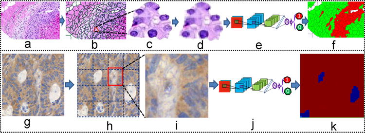
The illustration of DCNN+SMC approach for Epithelial and Stromal segmentation and classification for H&E (a–f) and IHC (g–k) stained histologic images. The original H&E (a) and IHC (g) stained images are over-segmented into sub-images using a SLIC (b) and fixed-size square window based approach (h), respectively. An exemplar patch (c) is resized into smaller 50 × 50 sub-images (d). The sub-images (d and i) are then fed to a DCNN (e and j) for segmentation and classification of epithelial and stromal regions, shown in panels (f) and (k), respectively. (For interpretation of the references to color in this figure caption, the reader is referred to the web version of this paper.)
The rest of this paper is organized as follows. A detailed description of DCNN is presented in Section 3. The experimental setup and comparative strategies are presented in Section 4. The experiment results and a discussion of the results are reported in Section 5. Concluding remarks are presented in Section 6.
3. Methods
3.1. The deep convolutional neural networks (DCNN)
The DCNN approach employed in this paper comprises two alternating convolutional layers (or layers, see Fig. 1(b)), max-pooling (or layers, see Fig. 1(c)), two full connection layers, and a final classification layer. The and layers produce a convolution and a max-pooling feature map via successive convolution and max-pooling operations, respectively. These feature maps then enable the extraction and combination of a set of appropriate image features from the training exemplars.
Fig. 1.
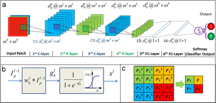
The architecture of the new DCNN employed in this work. The approach comprises of (a) two alternating convolutional layers (or -layers) with the convolutional operation (b) and max-pooling layers (or -layers) with the max-pooling operation, and (c) two full connection layers (or -layers), and an output layer.
3.2. The convolutional layer ( layer)
Let be a filter bank. Each , , is an ml × ml linear filter embedded in the l-th layer. is the number of different filters or kernels in the filter bank Wl. An input ωl−1 × ωl−1 patch is convolved with a ml × ml local receptive region in the image encompassed by the filter The filter moves over the input patch and allows for a local convolution operation. For each image patch extracted from the image, the convolutional operations with filters result in feature maps. The result of the linear convolutional operation on by can be re-written as . Here the pixel value gk(p) of each location of the resultant image is the sum of products of the filter coefficients and the image pixels of the local receptive region encompassed by the filter. During the convolutional operations, each filter wk convolves across (ωl−1−ml + 1) × (ωl−1−ml + 1) pixels in . The size of the resultant images is therefore (ωl−1−ml + 1) × (ωl−1−ml + 1) following the convolutional operation. is the pre-activation or input to the nonlinear activation function of a neuron. The output of the active function is . The procedure of convolu tional operation is illustrated in Fig. 1(b).
3.3. The max-pooling layer ( layers)
The max-pooling layers or layers aim to achieve spatial invariance by reducing the resolution of the feature maps obtained in layer . It applies local pooling of feature maps using a max operation in the neighbourhood of the results of the layer. The max-pooling operation in layers is described in Fig. 1(c). Subsequent to the max-pooling operation, the size of the resultant images becomes , where s refers to the scale at which the operation was applied.
3.4. Output layer: softmax classifier (SMC)
Softmax classifier (SMC) is a supervised model which generalizes logistic regression as
| (1) |
where is a sigmoid function with parameters W(l). The input xl of SMC is a high-level feature learned by the DCNN. The parameter W(l) corresponding to the SMC learned via a training set. With the learned parameter W(l), each patch that is fed to the function in Eq. (1) produces a value between 0 and 1 that can be interpreted as the probability of the input patch corresponding to either EP or ST. The predicted class and prediction score can then be represented as,
| (2) |
and
| (3) |
respectively.
3.5. Generating training and testing samples
Table 2 shows the number of training and testing images for the two data sets (D1 and D2) evaluated in this work. Additional details regarding to D1 and D2 are provided in Section 4.1.
Table 2.
The number of training and testing images as well as the corresponding training and testing patches for two superpixel methods (Ncut and SLIC) and sliding window approach for D1 and D2.
| Datasets | Total | Tissue | Training | Testing | |||||||||
|---|---|---|---|---|---|---|---|---|---|---|---|---|---|
| # of images | # of Sub-images | # of images | # of Sub-images | ||||||||||
| 80 × 80 | 50 × 50 | 80 × 80 | 50 × 50 | ||||||||||
| SLIC | Ncut | SW | SLIC | Ncut | SW | ||||||||
| D1 | NKI | 106 | Epithelial | 69 | 6763 | 6487 | 5296 | 37 | 3657 | 3386 | 2824 | ||
| Stromal | 6935 | 6461 | 5004 | 3607 | 3165 | 2659 | |||||||
| VGH | 51 | Epithelial | 36 | 4365 | 3967 | 3585 | 15 | 1612 | 1426 | 1475 | |||
| Stromal | 3606 | 3041 | 2779 | 1914 | 1340 | 1975 | |||||||
| D2 | 1376 | Epithelial | 401 | 15865 | 425 | 27820 | |||||||
| Stromal | 255 | 7169 | 295 | 10951 | |||||||||
For the segmentation of the epithelial and stromal compartments for the images in D1, the sub-images are generated with two superpixel approaches. The images corresponding to the training and testing sets within D1 and D2 are initially over-sesgmented into smaller tissue partitions by superpixel based algorithms [1,23]. Each tissue compartment is subsequently resized into 50 × 50 square sub-image patches via a bicubic interpolation approach [16]. The procedure for generating sub-images for the images from D1 is shown in Fig. 2(a)–(d). We use both the Ncut (Normalized cuts) [20,23] and SLIC (the Simple Linear Iterative Clustering) approach [1]. Our implementations are based on the source code provided in [20,23]. For comparison, we also employed a fixed-size SW approach for the images in D1. Each image in D1 is over-segmented into 50 × 50 sub-images using a sliding window. The window slides across the entire image row by row from the upper left corner to the lower right with a step size of 25 pixels. Border padding is employed to address issues of boundary artifacts.
For classification of the tissue compartments for the images in D2 we employ the approach in [19] to sub-divide the images into 80 × 80 square window images using a sliding window. A step size of 40 pixels is employed and as with D1. Also border padding is used to avoid boundary artifacts. The procedure for generating sub-images for images from D2 is shown in Fig. 2(g)–(i).
The sub-images in the training sets for D1 and D2 are used for training and optimizing the DCNN based and comparative models (see Table 3) while sub-images in the testing sets are used for qualitative and quantitative evaluations.
Table 3.
The illustration of models considered in the paper for comparison and the detailed description of the different models.
| Models | Feature extraction | Generating sub-images | Size of Sub-images | Classifier | ||
|---|---|---|---|---|---|---|
| D1 | D2 | D1 | D2 | |||
| Linder[19] | LBP+contrast measure | sliding window+square image | 50 × 50 | 80 × 80 | SVM | |
| Bianconi[6] | perception-based features | |||||
| Color-SW-SVM | pixel intensity | 50 × 50 | ||||
| DCNN-SW-SVM | DCNN | |||||
| DCNN-SW-SMC | SMC | |||||
| DCNN-Ncut+SMC | SP(Ncut)+square image | SMC | ||||
| DCNN-Ncut+SVM | SVM | |||||
| DCNN-SLIC+SVM | SP(SLIC)+square image | |||||
| DCNN-SLIC+SMC | SMC | |||||
4. Experimental Setup
In order to show the effectiveness of the approach, the DCNN and comparative models are qualitatively and quantitatively evaluated on D1 and D2, respectively.
4.1. Data set
4.1.1. Data set 1 (D1)
This data set was downloaded via the links provided in [4]. The data was acquired from two independent cohorts: Netherlands Cancer Institute (NKI) and Vancouver General Hospital (VGH). It consists of 157 rectangular image regions (106 NKI, 51 VGH) in which Epithelial and Stromal regions were manually annotated by pathologists. The images are H&E stained histologic images from breast cancer TMAs. The size of each image is 1128 × 720 pixels at a 20 × optical magnification.
4.1.2. Data set 2 (D2)
This data was downloaded from the links provided in [19]. The data was originally acquired at the Helsinki University Central Hospital from 1989 to 1998. D2 comprises 27 TMAs of colorectal cancer that were stained with epidermal growth factor receptor (EGFR) antibody and hematoxylin counterstain. The slides were digitized with a whole slide scanner under 20 × magnification. For the study, a total 1377 rectangular tissue samples of (826 EP and 451 ST) were chosen from 643 tumor cores. The tissue samples had been previously manually labeled as EP or ST by expert pathologists. The size of the annotations varied between 93 and 2372 pixels in width and 94-2373 in pixel height. As Table 2 shows, the image patches in both D1 and D2 were approximately evenly divided into training and testing subsets.
4.2. Training the DCNN
We used a coarse-to-fine sweep approach [27] to choose hyper-parameters for the DCNN. Our approach begins with a coarse setting (wide hyperparameter ranges, training only for 1–5 epochs), to more fine tuned settings (narrow ranges, training with many more epochs). The training procedure is based on the CAFFE framework [15].
4.3. Parameter setting
The flowchart illustrated in Fig. 2 is applied to both the comparative and DCNN-based approaches for tissue segmentation and classification. Note however that the different approaches differ in terms of the mechanism for feature extraction.
The parameter set for DCNN shown in Fig. 1 are as follows. , , m1 =m3 = 5, ω0 = 32, ω1 = 28, ω2 = 14, ω3 = 10, ω4 = 5. The max-pooling operation in the 2-nd and 4-th -layers involves searching over each 2 × 2 (s=2) neighborhood (see Fig. 1(c)). In L5, 50 feature maps of size 5 × 5 are fully connected with neurons. These 500 neurons are subsequently connected with neurons in L6. For the output layer, 100 neurons are fully connected with outputs.
We employ a greedy layer-wise approach [5] for training the DCNN by training each layer in a sequential manner. The trained SMC classifier yields an output based on Eq. (1). Based on Eq. (2), the class predicted for each input patch is either EP or ST .
4.4. Implementation of DCNN and SVM
All experiments were carried out on a PC (Intel Core(TM) 3.4 GHz processor with 16 GB of RAM) and a Quadro 2000 NVIDIA Graphics Processor Unit. The software implementation was performed using MATLAB 2014a. During the implementation, as Fig. 1 shows, we used two -Layers, 2 -Layers, two full connection layer ( -Layers), and an output layer. For the - and -Layers, a fixed 5 × 5 convolutional and 2 × 2 pooling kernel were used.
For the SVM classifier, we employed LIBSVM [7]. The Gaussian kernel was used and 10-fold cross-validation was employed for determining the parameters of the Gaussian kernel.
4.5. Experimental design
In the upper block in Fig. 2(b), the region with the red contour represents an atomic region generated by the SP algorithm. As DCNN requires uniformly sized sub-images as input, the atomic regions are then resized into 50 × 50 square image patches and subsequently fed to the DCNN for model training, segmentation, and classification. Applying this procedure to all atomic regions, the entire input image is classified as being either EP or ST via the DCNN + SMC classifier. For D2, the final classification of IHC patches is determined via the averaging of the confidence scores of all the sub-images in each patch.
For the SW based approach, each image pixel is usually segmented twice, the final segmentation result being determined as the most likely of the two segmentation results. To avoid bias in the evaluation process, we used the same image size (80 × 80) as described in [19] to extract sub-images in D2.
4.6. Comparative strategies
The DCNN based models and comparative strategies are shown in Table 3. A detailed description of the different models is illustrated in Table 3.
4.6.1. DCNN based models versus handcrafted features
We compared DCNN based approaches with extant handcrafted features used in [19,6]. For the color feature based approach (SW-color-SVM), we used color features which includes the color representation of pixel intensities in different color spaces. Linder [19] and Bianconi [6] described two state of art texture feature based approaches to classify EP and ST patches on D2, both of which are compared against our DCNN based model.
For D1, we implemented the LBP+Contrast measure [19]. Since the authors in [19] did not provide the source code, our implementation is based on the source code provided in [21], which appears to be the approach that inspired the work in [19]. We further compared DCNN+SMC against the approaches in [6] and [19] on D2. In order to compare the results of our version of the implementation in [21] the classification results reported in [6] and [19], we linearly mapped the results obtained by the softmax classifier for the approach we implemented based off [21] from [0,1] to [−3,3]. Based on Eqs. (2) and (3), the prediction confidence score is computed by
| (4) |
where is defined in (1). The confidence scores in Figs. 4 and 6 are the computed based on Eq. (4).
Fig. 4.
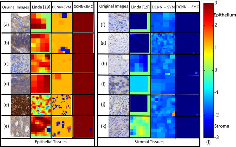
The probability maps rendered by the different DCNN based approaches (Columns 3 and 4) and [19] (in Column 2) for classifying EP ((a)–(e) in the left block, Column 1) and ST ((f)–(k) in the right block, Column 1) patches on D2. The false-color (defined by the heat map (l)) of sub-images in Columns 2–4 reflect the confidence score in predicting them as EP/ST regions via Linda [19], DCNN+SVM, and DCNN+SMC, respectively. The various colors in the heat map (l) correspond to the predicted confidence scores (red=EP with 100% likelihood and blue=ST with 100% likelihood). (For interpretation of the references to color in this figure caption, the reader is referred to the web version of this paper.)
Fig. 6.
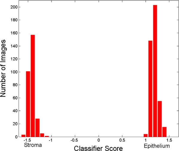
A plot of the score value on the X-axis versus the number of image patches on the Y-axis for the model DCNN-SW-SVM on dataset D2.
4.6.2. Evaluating DCNN across different sub-image generation methods
We compared the SP algorithm with fixed-size SW scheme for generating the sub-images. Also, in order to show the performance of different SP algorithms in terms of generation of the sub-images, we applied two popular algorithms: Ncut [23] and SLIC [1] for generating the atomic regions.
4.6.3. Evaluating DCNN with different supervised classifiers
In order to show the efficiency of DCNN for learning high-level feature, we compared the performance of DCNN coupling to different machine learning classifiers. We compared the DCNN+SMC with the DCNN+SVM. For the DCNN+SVM model, we first trained the DCNN+SMC model with training data. The model parameters for the DCNN model were thus learnt and then fixed for the testing phase. The output of the DCNN was then fed to a Support Vector Machine (SVM) classifier which was then further trained with sub-images in the training set.
4.6.4. Evaluating the effect of window size on the DCNN
The segmentation accuracy of the DCNN+SMC model was determined in terms of ROC curves, generated across all the test images in D1 as a function of the window size.
The performance of the automated segmentation and classification approaches provided by different models is quantified in terms of measurements [22] shown in Table 1. The Receiver Operating Characteristic (ROC) curves are also drawn to assess the classification performance provided by the different models.
Table 1.
Enumeration of the symbols used in the paper.
| Symbol | Description | Symbol | Description |
|---|---|---|---|
| DCNN | Deep Convolutional Neural Networks | SMC | Softmax classifier |
| EP | Epithelial region | ST | Stromal region |
| LBP | Local Binary Patterns | SVM | Support Vector Machine |
| F1 | F1 score | ACC | Accuracy |
| TP | True Positive | FP | False positive |
| FN | False Negative | TN | True negative |
| MCC | Matthews Correlation Coefficient | ROC | Receiver Operating Characteristic |
| TMAs | Tumor tissue microarrays | IHC | Immunohistochemistry |
| H&E | Hematoxylin and Eosin | DL | Deep learning |
| SP | Superpixel | SW | Sliding window |
| layer | Convolutional layer | layer | max-pooling layer |
| layer | Full connection layer | ROI | Region of interest |
| D1 | Dataset 1 | D2 | Dataset 2 |
| NKI | Netherlands Cancer Institute Dataset | VGH | Vancouver General Hospital Dataset |
| SLIC | Simple Linear Iterative Clustering algorithm | Ncut | Normalized cuts algorithm |
| DCNN+SMC | DCNN plus SMC | DCNN+SVM | DCNN plus SVM |
5. Experimental results and discussion
5.1. Qualitative results
The qualitative segmentation results of the DCNN (Fig. 3(c)–(h)) and color feature extraction based (Fig. 3(i)) models for a histological image in D1 (Fig. 3(a)) are shown in Fig. 3. In Fig. 3(b)–(i), green and red regions represent epithelial and stromal regions that were accurately segmented with respect to the pathologist determined ground truth (Fig. 3(b)). The black areas in Fig. 3(b)–(i) were identified as background regions and hence not worth computationally interrogating. As the qualitative results in Fig. 3(c)–(h) suggest, the segmentation results from the SP-based methods are visually different from the SW-based methods which were prone to producing zigzag boundaries while the SP-based methods produced natural boundaries. Although SP-based methods produced erroneous boundaries as well, the errors appeared more subtle and less egregious, possibly since the superpixel based algorithms represent a natural partitioning of visual scenes. The results of pixel-wise classification on EP (Fig. 4(a)–(e)) and ST (Fig. 4(f)–(k)) patches in D2 are shown in Fig. 4. In Fig. 4(a)–(k), the colors in the heat map (i) correspond to the predicted confidence scores (red=EP with 100% and blue=ST with 100%). The results in Fig. 3 appear to suggest that DCNN based models outperform handcrafted feature extraction based models. Also, DCNN+SMC appears to outperform DCNN+SVM.
Fig. 3.
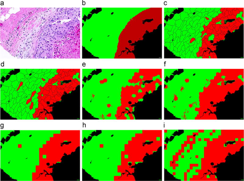
Segmentation of epithelial (red) and stromal (green) regions on a tissue image (a) using the different segmentation approaches on D1. (b) The ground truth (a) annotations of stromal and epithelial regions by an expert pathologist. The classification results are shown for DCNN-Ncut-SVM (c), DCNN-Ncut-SMC (d), DCNN-SLIC-SVM (e), DCNN-SLIC-SMC (f), DCNN-SW-SVM (g), DCNN-SW-SMC (h), and Color-SW-SVM (i), respectively. (For interpretation of the references to color in this figure caption, the reader is referred to the web version of this paper.)
5.2. Quantitative results
The quantitative performance for tissue segmentation and classification for the different models on D1 and D2 are shown in Table 4. The DCNN based approach yields a perfect result (100%) in terms of True Positive Rate (TPR), True Negative Rate (TNR), Positive Predictive Value (PPV), Negative Predictive Value (NPV), Accuracy (ACC), F1 Score (F1), and Matthews Correlation Coefficient (MCC) and outperforms the approaches described in [6] and [19] respectively. Fig. 5(a) and (b) shows the ROC curves corresponding to segmentation accuracy for DCNN-Ncut-SMC, DCNN-SLIC-SMC, DCNN-Ncut-SVM, DCNN-SLIC-SVM, DCNN-SW-SVM, Color-SW-SVM, Linda [19] on NKI (Fig. 5(a)) and VGH ((Fig. 5(b)) of D1. The AUC values suggest that the DCNN based models outperform the handcrafted feature based approaches (Color-SW-SVM model and approaches in [19]), with the DCNN-Ncut-SVM is emerging as marginally better than the other models. Fig. 6 shows the histogram for the DCNN-SW-SVM model for EP and ST patch based classification for D2. Fig. 6 is a plot of number of images (Y-axis) versus the confidence score (X-axis) for the SVM classifier. The two types of image patches appear to be well separated. Finally, in terms of the comparison between two different SP algorithms, Table 4 shows that the performance of Ncut is slightly better than SLIC on D1. Additionally, the SVM classifier slightly outperforms SMC on D1.
Table 4.
The quantitative evaluation of segmentation and classification results on D1 and D2 with different models. The bolded numbers reflect the best performance for a specific performance measure within the data set.
| Models | Datasets | TPR (%) | TNR (%) | PPV (%) | NPV (%) | FPR (%) | FDR (%) | FNR (%) | ACC (%) | F1 (%) | MCC (%) | |
|---|---|---|---|---|---|---|---|---|---|---|---|---|
| Linda[19] | D1 | NKI | 46.60 | 90.14 | 83.82 | 60.64 | 9.86 | 16.18 | 53.40 | 67.39 | 59.90 | 40.41 |
| VGH | 97.29 | 41.64 | 66.18 | 92.92 | 58.36 | 33.82 | 2.71 | 71.69 | 78.77 | 47.96 | ||
| D2 | 98.64 | 95.53 | 93.87 | 99.02 | 4.47 | 6.13 | 1.36 | 96.84 | 96.20 | 93.53 | ||
| Bianconi[6] | D1 | NKI | ||||||||||
| VGH | ||||||||||||
| D2 | 95.25 | 98.12 | 97.23 | 96.75 | 1.88 | 2.77 | 4.75 | 96.94 | 96.23 | 93.68 | ||
| DCNN-SW-SVM | D1 | NKI | 70.40 | 93.87 | 92.63 | 74.33 | 6.13 | 7.37 | 29.60 | 81.60 | 80.00 | 65.60 |
| VGH | 87.01 | 82.20 | 85.15 | 84.36 | 17.80 | 14.85 | 12.99 | 84.79 | 86.07 | 69.36 | ||
| D2 | 100 | 100 | 100 | 100 | 0 | 0 | 0 | 100 | 100 | 100 | ||
| Color-SW-SVM | D1 | NKI | 89.86 | 58.59 | 70.40 | 84.05 | 41.41 | 29.60 | 10.14 | 74.94 | 78.95 | 51.36 |
| VGH | 86.69 | 66.42 | 75.19 | 80.95 | 33.59 | 24.81 | 13.31 | 77.36 | 80.53 | 54.60 | ||
| D2 | ||||||||||||
| DCNN-SW-SMC | D1 | NKI | 77.95 | 80.68 | 81.63 | 76.86 | 19.32 | 18.37 | 22.05 | 79.25 | 79.75 | 58.56 |
| VGH | 82.18 | 86.12 | 87.46 | 80.40 | 13.88 | 12.54 | 17.82 | 83.99 | 84.74 | 68.08 | ||
| D2 | ||||||||||||
| DCNN-Ncut-SVM | D1 | NKI | 81.09 | 86.39 | 86.71 | 80.67 | 13.61 | 13.27 | 18.91 | 83.62 | 83.81 | 67.43 |
| VGH | 88.29 | 88.40 | 89.93 | 86.55 | 11.60 | 10.07 | 11.71 | 88.34 | 89.10 | 76.59 | ||
| D2 | ||||||||||||
| DCNN-Ncut-SMC | D1 | NKI | 88.92 | 67.94 | 75.23 | 84.85 | 32.06 | 24.77 | 11.08 | 78.91 | 81.05 | 58.45 |
| VGH | 89.37 | 86.63 | 88.67 | 87.42 | 13.37 | 11.31 | 10.63 | 88.11 | 89.03 | 76.05 | ||
| D2 | ||||||||||||
| DCNN-SLIC-SVM | D1 | NKI | 80.63 | 85.79 | 86.13 | 80.18 | 14.21 | 13.87 | 19.37 | 83.09 | 83.29 | 66.37 |
| VGH | 88.51 | 83.68 | 86.41 | 86.13 | 16.32 | 13.59 | 11.49 | 86.28 | 87.45 | 72.36 | ||
| D2 | ||||||||||||
| DCNN-SLIC-SMC | D1 | NKI | 86.31 | 82.15 | 84.11 | 84.60 | 17.85 | 15.89 | 13.66 | 84.34 | 85.21 | 68.60 |
| VGH | 87.88 | 82.13 | 85.22 | 85.25 | 17.87 | 14.78 | 12.12 | 85.23 | 86.53 | 70.24 | ||
| D2 | ||||||||||||
Fig. 5.
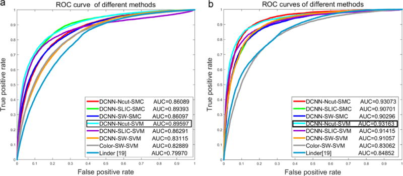
The ROC curves for the different models (see Table 3) for detecting EP and ST regions on NKI (a) and VGH (b) data cohorts within D1.
5.3. Sensitivity analysis
Fig. 7 shows the sensitivity of window size (X-axis) on the segmentation accuracy (Y-axis) for the DCNN-SW-SVM model D1. Fig. 7 suggests that the DCNN-SW-SVM model achieves the best AUC value when the window size is around 50 × 50 pixels. As a result, we chose a window size of 50 × 50 for all our subsequent experiments.
Fig. 7.
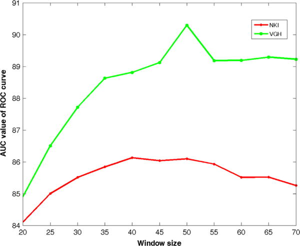
Plot of AUC versus window size for the DCNN-SW-SVM model on NKI and VGH datasets within D1.
6. Concluding remarks
In this paper we presented a new Deep Convolutional Neural Network (DCNN) based model for segmentation and classification of epithelial and stromal regions within Hematoxylin and Eosin (H & E) and Immunohistochemistry (IHC) images of breast and colon cancer. DCNN uses a deep architecture to learn complex features in a data-driven fashion and that has been shown in multiple applications outperform the classification accuracy obtained via handcrafted features. We compared the DCNN based models with extant handcrafted features and showed that for the task of separating stroma from epithelium, the DCNN based models consistently outperformed handcrafted features based models. Future work will entail evaluation of our approach on tissue partitioning for other types of cancers as well.
Acknowledgments
Research reported in this publication was supported by National Natural Science Foundation of China (No. 61273259); Six Major Talents Summit of Jiangsu Province (No. 2013-XXRJ-019), and Natural Science Foundation of Jiangsu Province of China (No. BK20141482); Jiangsu Innovation & Entrepreneurship Group Talents Plan; the National Cancer Institute of the National Institutes of Health under award numbers R01CA136535-01, R01CA140772-01, R21CA167811-01, R21CA179327-01; the National Institute of Diabetes and Digestive and Kidney Diseases under award number R01DK098503-02, the DOD Prostate Cancer Synergistic Idea Development Award (PC120857); the DOD Lung Cancer Idea Development New Investigator Award (LC130463), the Ohio Third Frontier Technology development Grant, the CTSC Coulter Annual Pilot Grant, and the Wallace H. Coulter Foundation Program in the Department of Biomedical Engineering at Case Western Reserve University.
Biographies

Jun Xu received his M.S. degree in Applied Mathematics from the University of Electronic Science and Technology of China, Chengdu, China, in 2004, and the Ph.D. degree in Control Science and Engineering from the Zhejiang University, Hangzhou, China, in 2007. From 2008 to 2011, he had been a postdoctoral associate and research assistant at Department of Biomedical Engineering, Rutgers University, USA. In the summer of 2014, he had been a Visiting Assistant Professor at Department of Biomedical Engineering, Case Western Reserve University, USA. He is currently a full professor at School of Information & Control, Nanjing University of Information Science and Technology, China. His research interests include medical image analysis, computer vision, machine learning, digital pathology, and computer-aided detection, diagnosis, and prognosis on cancer. He authored more than thirty papers in various leading international journals and conferences. His research work has received grant funding from National Science Foundation of China.
Xiaofei Luo received the B.S. degrees from the Nanjing University of Information Science and Technology, Nanjing, China, in 2013. He is currently working toward the M.S. degree in the School of Information and Control, Nanjing University of Information Science and Technology. His current research interests is machine learning and its application in computer-aided diagnosis on cancers.
Guanhao Wang received his B.S. and M.S. degrees from the Nanjing University of Information Science and Technology, Nanjing, China, in 2012 and 2015, respectively. His research interest is pattern recognition. He is now working at Novatek Inc. in Shanghai, China.

Hannah Gilmore MD is the Director of Surgical Pathology and Director of the Breast Pathology Service at University Hospitals Case Medical Center. She is an Assistant Professor in the Department of Pathology at Case Western Reserve University and is a member of the Case Comprehensive Cancer Center. She is a clinical expert in the diagnosis of breast diseases and is a member of the College of American Pathologists Advanced Multidisciplinary Breast Program. Gilmores research in breast disease spans the clinical, translational and basic science spectrum and has been published in numerous peer-reviewed journals. In addition to receiving research and teaching awards, her work has been funded by the National Cancer Institute, the Department of Defense, the American Cancer Society as well as from Industry.

Anant Madabhushi is the Director of the Center for Computational Imaging and Personalized Diagnostics (CCIPD) and a Professor in the Departments of Biomedical Engineering, Pathology, Radiology, Radiation Oncology, Urology, General Medical Sciences, and Electrical Engineering and Computer Science at Case Western Reserve University. Madabhushi has authored over 240 peer-reviewed publications in leading international journals and conferences. He has 10 issued patents with over 20 patents pending in the areas of medical image analysis, computer-aided diagnosis, and computer vision. He is an Associate Editor for IEEE Transactions on Biomedical Engineering, IEEE Transactions on Biomedical Engineering Letters, BMC Cancer, BMC Medical Imaging, Journal of Medical Imaging and Medical Image Analysis (MedIA). He is also on the Editorial Board of the Journal Analytical and Cellular Pathology. He has been the recipient of a number of awards for both research as well as teaching, including the Department of Defense New Investigator Award in Lung Cancer (2014), the Coulter Phase 1 and Phase 2 Early Career award (2006, 2008), and the Excellence in Teaching Award (2007–2009), along with a number of technology commercialization awards. He is also a Wallace H. Coulter Fellow, a Fellow of the American Institute of Medical and Biological Engineering (AIMBE), and a Senior IEEE member. In 2015 he was named by Crains Cleveland Business Magazine as one of Forty under 40 making positive impact to business in North East Ohio. His research work has received grant funding from the National Cancer Institute (NIH), National Science Foundation, the Department of Defense, private foundations, and from Industry.
He is also the co-founder of Ibris Inc. a startup company focused on developing image based assays for breast cancer prognosis. He is also the conference chair for the new Digital Pathology Conference to be held annually in conjunction with the SPIE Medical Imaging Symposium.
References
- 1.Achanta R, Shaji A, Smith K, Lucchi A, Fua P, Susstrunk S. SLIC superpixels compared to state-of-the-art superpixel methods. IEEE Trans Pattern Anal Mach Intell. 2012;34(11):2274–2282. doi: 10.1109/TPAMI.2012.120. [DOI] [PubMed] [Google Scholar]
- 2.Ali S, et al. Spatially aware cell clusters graphs: predicting outcome in HPV associated oropharyngeal tumors. Medical Image Computing and Computer-Assisted Intervention. 2013;8149:412–519. doi: 10.1007/978-3-642-40811-3_52. [DOI] [PubMed] [Google Scholar]
- 3.Amaral T, McKenna S, Robertson K, Thompson A. Classification and immunohistochemical scoring of breast tissue microarray spots. IEEE Trans Biomed Eng. 2013 Oct;60(10):2806–2814. doi: 10.1109/TBME.2013.2264871. [DOI] [PubMed] [Google Scholar]
- 4.Beck AH, et al. Systematic analysis of breast cancer morphology uncovers stromal features associated with survival. Sci Transl Med. 2011;3:108ra113. doi: 10.1126/scitranslmed.3002564. [DOI] [PubMed] [Google Scholar]
- 5.Bengio Y, Lamblin P, Popovici D, Larochelle H, et al. Greedy layer-wise training of deep networks. Adv Neural Inf Process Syst. 2007;19:153. [Google Scholar]
- 6.Bianconi F, lvarez Larrn A, Fernndez A. Discrimination between tumour epithelium and stroma via perception-based features. Neurocomputing. 2015;154(0):119–126. 〈 http://www.sciencedirect.com/science/article/pii/S0925231214016762〉. [Google Scholar]
- 7.Chang CC, Lin CJ. LIBSVM: a library for support vector machines. ACM Trans Intell Syst Technol. 2011;2:27:1–27:27. software available at URL 〈 http://www.csie.ntu.edu.tw/~cjlin/libsvm〉. [Google Scholar]
- 8.Chang H, Zhou Y, Borowsky A, Barner K, Spellman P, Parvin B. Stacked predictive sparse decomposition for classification of histology sections. Int J Comput Vis. 2015;113(1):3–18. doi: 10.1007/s11263-014-0790-9. URL 〈 http://dx.doi.org/10.1007/s11263-014-0790-9〉. [DOI] [PMC free article] [PubMed] [Google Scholar]
- 9.Ciresan DC, et al. Medical Image Computing and Computer-Assisted Intervention (MICCAI 2013) Vol. 8150. Springer; Nagoya, Japan: 2013. Mitosis detection in breast cancer histology images with deep neural networks; pp. 411–418. (Lecture Notes in Computer Science). [DOI] [PubMed] [Google Scholar]
- 10.Cruz-Roa A, et al. Medical Image Computing and Computer-Assisted Intervention (MICCAI 2013) Vol. 8150. Springer; Nagoya, Japan: 2013. A deep learning architecture for image representation, visual interpretability and automated basal-cell carcinoma cancer detection; pp. 403–410. [DOI] [PubMed] [Google Scholar]
- 11.De Wever O, Mareel M. Role of tissue stroma in cancer cell invasion. J Pathol. 2003;200(4):429–447. doi: 10.1002/path.1398. [DOI] [PubMed] [Google Scholar]
- 12.Downey CL, Simpkins SA, White J, Holliday DL, Jones JL, Jordan LB, Kulka J, Pollock S, Rajan SS, Thygesen HH, Hanby AM, Speirs V. The prognostic significance of tumour-stroma ratio in oestrogen receptor-positive breast cancer. Br J Cancer. 2014 Apr;110(7):1744–1747. doi: 10.1038/bjc.2014.69. URL 〈 http://dx.doi.org/10.1038/bjc.2014.69〉. [DOI] [PMC free article] [PubMed] [Google Scholar]
- 13.Eramian M, et al. Segmentation of epithelium in H&E stained odontogenic cysts. J Microsc. 2011;244(3):273–292. doi: 10.1111/j.1365-2818.2011.03535.x. [DOI] [PubMed] [Google Scholar]
- 14.Hiary H, et al. Automated segmentation of stromal tissue in histology images using a voting Bayesian model. Signal Image Video Process. 2013;7(6):1229–1237. URL 〈 http://dx.doi.org/10.1007/s11760-012-0393-2〉. [Google Scholar]
- 15.Jia Y, Shelhamer E, Donahue J, Karayev S, Long J, Girshick R, Guadarrama S, Darrell T. Caffe: convolutional architecture for fast feature embedding. 2014 arXiv preprint arxiv:1408.5093. [Google Scholar]
- 16.Keys R. Cubic convolution interpolation for digital image processing. IEEE Trans Acoust Speech Signal Process. 1981 Dec;29(6):1153–1160. [Google Scholar]
- 17.Lahrmann B, Halama N, Sinn HP, Schirmacher P, Jaeger D, Grabe N. Automatic tumor-stroma separation in fluorescence TMAs enables the quantitative high-throughput analysis of multiple cancer biomarkers. PLoS One. 2011 Dec;6(12):e28048. doi: 10.1371/journal.pone.0028048. [DOI] [PMC free article] [PubMed] [Google Scholar]
- 18.LeCun Y, Bengio Y, Hinton G. Deep learning. Nature. 2015 May;521(7553):436–444. doi: 10.1038/nature14539. URL 〈 http://dx.doi.org/10.1038/nature14539〉. [DOI] [PubMed] [Google Scholar]
- 19.Linder N, et al. Identification of tumor epithelium and stroma in tissue microarrays using texture analysis. Diagn Pathol. 2012;7(1):22. doi: 10.1186/1746-1596-7-22. URL 〈 http://www.diagnosticpathology.org/content/7/1/22〉. [DOI] [PMC free article] [PubMed] [Google Scholar]
- 20.Madabhushi A, Shi J, Rosen M, Tomaszeweski J, Feldman M. Graph embedding to improve supervised classification and novel class detection: application to prostate cancer. In: Duncan J, Gerig G, editors. Medical Image Computing and Computer-Assisted Intervention? MICCAI 2005. Vol. 3749. Springer; Berlin, Heidelberg: 2005. pp. 729–737. (Lecture Notes in Computer Science). [DOI] [PubMed] [Google Scholar]
- 21.Ojala T, Pietikainen M, Maenpaa T. Multiresolution gray-scale and rotation invariant texture classification with local binary patterns. IEEE Trans Pattern Anal Mach Intell. 2002 Jul;24(7):971–987. [Google Scholar]
- 22.Powers D. Technical Report. Adelaide, Australia: 2007. Evaluation: from Precision, Recall and F-factor to ROC, Informedness, Markedness & Correlation. [Google Scholar]
- 23.Ren X, Malik J. Learning a classification model for segmentation. International Conference on Computer Vision (ICCV 2003) 2003;1:10–17. [Google Scholar]
- 24.Shi J, Malik J. Normalized cuts and image segmentation. IEEE Trans Pattern Anal Mach Intell. 2000;22(8):888–905. [Google Scholar]
- 25.Su H, Xing F, Kong X, Xie Y, Zhang S, Yang L. Robust cell detection and segmentation in histopathological images using sparse reconstruction and stacked denoising autoencoders. In: Navab N, Hornegger J, Wells W, Frangi A, editors. Medical Image Computing and Computer-Assisted Intervention: MICCAI 2015. Vol. 9351. Springer International Publishing; Munich, Germany: 2015. pp. 383–390. (Lecture Notes in Computer Science). [DOI] [PMC free article] [PubMed] [Google Scholar]
- 26.Wang H, et al. Mitosis detection in breast cancer pathology images by combining handcrafted and convolutional neural network features. J Med Imaging. 2014;1(3):034003. doi: 10.1117/1.JMI.1.3.034003. URL 〈 http://dx.doi.org/10.1117/1.JMI.1.3.034003〉. [DOI] [PMC free article] [PubMed] [Google Scholar]
- 27.Weller DS, Ramani S, Nielsen JF, Fessler JA. Monte carlo sure-based parameter selection for parallel magnetic resonance imaging reconstruction. Magn Reson Med. 2014;71(5):1760–1770. doi: 10.1002/mrm.24840. [DOI] [PMC free article] [PubMed] [Google Scholar]
- 28.Xu J, Xiang L, Hang R, Wu J. 2014 IEEE 11th International Symposium on Biomedical Imaging (ISBI) IEEE; Beijing, China: 2014. Stacked sparse autoencoder (SSAE) based framework for nuclei patch classification on breast cancer histopathology; pp. 999–1002. [Google Scholar]
- 29.Xu J, Xiang L, Liu Q, Gilmore H, Wu J, Tang J, Madabhushi A. Stacked sparse autoencoder (SSAE) for nuclei detection on breast cancer histopathology images. IEEE Trans Med Imaging. 2016 Jan;35(1):119–130. doi: 10.1109/TMI.2015.2458702. [DOI] [PMC free article] [PubMed] [Google Scholar]
- 30.Xu J, Xiang L, Wang G, Ganesan S, Feldman M, Shih NN, Gilmore H, Madabhushi A. Sparse non-negative matrix factorization (SNMF) based color unmixing for breast histopathological image analysis. Comput Med Imaging Graph. 2015;46(Part 1):20–29. doi: 10.1016/j.compmedimag.2015.04.002. sparsity Techniques in Medical Imaging. URL 〈 http://www.sciencedirect.com/science/article/pii/S0895611115000774〉. [DOI] [PubMed] [Google Scholar]
- 31.Yuan Y, et al. Quantitative image analysis of cellular heterogeneity in breast tumors complements genomic profiling. Sci Transl Med. 2012;4(157):157ra143. doi: 10.1126/scitranslmed.3004330. [DOI] [PubMed] [Google Scholar]
- 32.Zhang X, Liu W, Dundar M, Badve S, Zhang S. Towards large-scale histopathological image analysis: hashing-based image retrieval. IEEE Trans Med Imaging. 2015 Feb;34(2):496–506. doi: 10.1109/TMI.2014.2361481. [DOI] [PubMed] [Google Scholar]
- 33.Zhang X, Liu W, Zhang S. Mining histopathological images via hashing-based scalable image retrieval. 2014 IEEE 11th International Symposium on Biomedical Imaging (ISBI) 2014 Apr;:1111–1114. [Google Scholar]
- 34.Zhang X, Su H, Yang L, Zhang S. Fine-grained histopathological image analysis via robust segmentation and large-scale retrieval. IEEE Conference on Computer Vision and Pattern Recognition (CVPR) 2015 Jun; [Google Scholar]


