Biostatistics Series Module 7: The Statistics of Diagnostic Tests

Abstract

Crucial therapeutic decisions are based on diagnostic tests. Therefore, it is important to evaluate such tests before adopting them for routine use. Although things such as blood tests, cultures, biopsies, and radiological imaging are obvious diagnostic tests, it is not to be forgotten that specific clinical examination procedures, scoring systems based on physiological or psychological evaluation, and ratings based on questionnaires are also diagnostic tests and therefore merit similar evaluation. In the simplest scenario, a diagnostic test will give either a positive (disease likely) or negative (disease unlikely) result. Ideally, all those with the disease should be classified by a test as positive and all those without the disease as negative. Unfortunately, practically no test gives 100% accurate results. Therefore, leaving aside the economic question, the performance of diagnostic tests is evaluated on the basis of certain indices such as sensitivity, specificity, positive predictive value, and negative predictive value. Likelihood ratios combine information on specificity and sensitivity to expresses the likelihood that a given test result would occur in a subject with a disorder compared to the probability that the same result would occur in a subject without the disorder. Not all test can be categorized simply as “positive” or “negative.” Physicians are frequently exposed to test results on a numerical scale, and in such cases, judgment is required in choosing a cutoff point to distinguish normal from abnormal. Naturally, a cutoff value should provide the greatest predictive accuracy, but there is a trade-off between sensitivity and specificity here - if the cutoff is too low, it will identify most patients who have the disease (high sensitivity) but will also incorrectly identify many who do not (low specificity). A receiver operating characteristic curve plots pairs of sensitivity versus (1 − specificity) values and helps in selecting an optimum cutoff – the one lying on the “elbow” of the curve. Cohen's kappa (κ) statistic is a measure of inter-rater agreement for categorical variables. It can also be applied to assess how far two tests agree with respect to diagnostic categorization. It is generally thought to be a more robust measure than simple percent agreement calculation since kappa takes into account the agreement occurring by chance.

Introduction

Clinical practice makes use of numerous diagnostic tests, some for screening, and some for confirmation of disease. Since crucial therapeutic decisions will often be based on diagnostic tests, it is important for clinicians to understand the strengths and limitations of every test they use. Therefore, every new test or a new application of an existing test needs to be evaluated against some gold standard. Although things such as blood tests, biopsies, cultures, and radiological investigations are obvious diagnostic tests, it is to be borne in mind that specific clinical examination procedures, scoring systems based on physiological or psychological evaluation, and ratings based on questionnaires are also diagnostic tests and therefore merit similar evaluations before application to a wide spectrum of subjects.

In the simplest scenario, a diagnostic test should give either a positive or negative result or a reading that makes disease either likely or unlikely. In an ideal world, all those with disease should be categorized by the test as positive and all those without the disease as negative. Unfortunately, few diagnostic tests will give 100% accurate results. Therefore, leaving aside the economic question, the performance of diagnostic tests is evaluated on the basis of a number of indices.

Accuracy versus Precision

Accuracy (also called validity) is the degree of conformity of a measured or calculated quantity to its actual or true value. Precision denotes the degree of mutual agreement or repeatability among a series of measurements or calculations under similar conditions.

An analogy often used to explain accuracy and precision in the context of repeated measurements is the firing of shotgun pellets at a target [Figure 1]. Accuracy signifies the proximity of the shots to the bullseye at the center of the target. Pellets that strike closer to the bullseye would be considered more accurate. Precision would be signified by the size of the pellet cluster. When the shots are grouped tightly together, the cluster is considered precise since the shots all struck close to the same spot, but not necessarily near the bullseye. If the cluster is close to the bullseye, the shots are accurate as well as precise; if not they are precise but not accurate. However, it is not possible to achieve a high degree of accuracy without precision - if the shots are not grouped close to one another, they cannot all be close to the bullseye.

Figure 1.

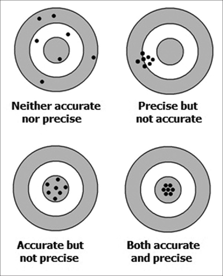
The concept of accuracy versus precision

Like measurements, diagnostic tests too need to be both accurate and precise to a sufficient degree to be acceptable. The accuracy and precision of a measurement process are usually established by repeatedly measuring a reference standard. The accuracy may be quantified as the difference between the mean of the measurements and the reference value - the bias. Establishing and correcting for bias are necessary for calibration of the test. Precision is usually characterized in terms of the standard error of the measurements.

Precision is sometimes stratified into:

• Repeatability: The variation possible when all efforts are made to keep conditions constant using the same instrument and operator and repeating during a short period

• Reproducibility: The variation possible using the same measurement process among different instruments and operators and over longer time periods.

Robustness

Diagnostic tests and procedures require us to assume that specific conditions are met during testing. Given that these conditions are met, the tests will return accurate and reliable results. In practice, however, testing will often be carried out in conditions which deviate to some extent from ideal conditions. A test would be considered to be robust if it still returns valid results despite these variations, provided of course that the variations are not too large.

Sensitivity, Specificity, Predictive Values, and Likelihood Ratios

These are a standard set of performance criteria for any diagnostic test that returns a dichotomous (positive or negative) result.

Sensitivity denotes the probability of a positive test result when disease is present. It is calculated as the percentage of individuals with a disease who are correctly categorized as having the disease. A test would be considered sensitive, in general if it is positive for most individuals having the disease.

Specificity denotes the probability of a negative test result when disease is absent. It is calculated as the percentage of individuals without the disease who are correctly categorized as not having the disease. A test would be considered specific, in general, if it is positive for only a small fraction of those without the disease.

In a nutshell, sensitivity of a test is the true positive rate while specificity is the true negative rate. Obviously, we would like to have a test that is both highly sensitive as well as specific, i.e., both sensitivity and specificity values close to 100%. Unfortunately, we cannot have the best of both worlds, and, in practice, we gain sensitivity at the expense of specificity and vice versa. Whether or not, we aim for a high sensitivity or a high specificity depends on the disease in question and the clinical and socioeconomic implications of the result for the subject and the society. For conditions that are readily treatable, we would prefer tests with the maximum possible sensitivity, whereas if the treatment is likely to be toxic or expensive, we would prefer high specificity to avoid treating a subject who actually does not have the disease. If the disease is serious, then we may adopt the strategy of using screening tests of high sensitivity and then confirming the diagnosis with highly specific confirmatory tests before initiating treatment. This is the typical scenario in the diagnosis of HIV/AIDS, where an ELISA test of high sensitivity is used for screening, and then, a Western blot of high specificity is used for confirming the diagnosis in ELISA-positive cases.

Positive predictive value (PPV) denotes the probability of disease being present when test is positive and is calculated as the percentage of individuals with positive test result who actually have the disease.

Negative predictive value (NPV) denotes the probability of disease being absent when test is negative and is calculated as the percentage of individuals with negative test result who are actually free from disease.

Predictive values enable us to summarize how likely an individual is in having or not having a disease given the test result. They are dependent on the prevalence of the disease in the underlying population. If the disease is common, the PPV of a given test would be higher than in a population where the disease is uncommon. The inverse is true for NPV.

We can derive the formulas for the above performance indicators from the following cross-tabulation.

• Sensitivity = a/(a + c)

• Specificity = d/(b + d)

• PPV = a/(a + b)

• NPV = d/(c + d).

Note that, we can consider a, b, c, and d as the number of true positive, false positive, false negative, and true negative results, respectively.

We can summarize information about a diagnostic test using a measure called the likelihood ratio (LR) that combines information about the sensitivity and specificity. It tells us how much a positive or negative test result changes the likelihood that a subject would have the disease.

• The LR of a positive test result (LR+) is sensitivity/(1 − specificity)

• The LR of a negative test result (LR−) is (1 − sensitivity)/specificity.

Thus, this index expresses the likelihood that a given test result would be expected in a patient with a certain disorder compared to the likelihood that the same result would occur in a patient without the disorder. For instance, the positive LR of computerized tomography (CT) scan in the diagnosis of acute appendicitis (sensitivity 94% and specificity 95%) is considered to be about +18.8; this indicates that an individual is about 19 times as likely to have CT scan finding positive when they do have acute appendicitis than when they do not have acute appendicitis. Thus, a positive CT scan in a patient presenting with clinical signs and symptoms suggestive of acute appendicitis indicates a very strong likelihood (any LR> +10 is considered to indicate strong likelihood that the diagnosis is correct). On the other hand, the LR − for CT scan in acute appendicitis is 0.06, which indicates that there is minimum likelihood of the disease being present when the test is negative. For ultrasonography (USG) in the diagnosis of acute appendicitis (sensitivity 86% and specificity 81%), the LR+ and LR− figures are 4.5 and 0.17 respectively. Note that the decision to order a test is also based on the initial assessment of the likelihood of the disease in question and how important it is to rule-in or rule-out disease. For example, a CT scan might have a good LR for ruling in (or out) appendicitis in a child with abdominal pain, but if the physician believes that the child has simple abdominal colic and that appendicitis is very unlikely, CT should not be ordered given the cost and radiation exposure involved. Hence, beginning with ultrasound and only getting CT if the results remain unclear or if the patient does not improve is a more prudent option. The issue of prior probability of a disease and its contribution to ultimate clinical interpretation, combining with the LR information, merits extensive discussion which we will leave for the future.

It is to be noted that LR, when stated without qualification as to positive or negative, usually indicates the LR of a positive test result.

To illustrate the above performance indicators, consider this example. Testing for HLA-DR3 in blood has been proposed as a screening test for psoriasis in adults over 50 years age. Here are the results when applied to 203 subjects.

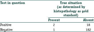
• Sensitivity = 2/(2 + 1) = 66.67%

• Specificity = 182/(18 + 182) = 91.00%

• PPV = 2/(2 + 18) = 10.00%

• NPV = 182/(1 + 182) = 99.45%

• LR+ = Sensitivity/(1 − specificity) =66.67%/(1 − 91%) = 7.40

• LR− = (1 − sensitivity)/specificity = (1 − 66.67%)/91% = 0.37.

Here, with the relatively large numbers of false positives and few false negatives, a positive HLA-DR3 test result is in itself poor at confirming psoriasis (PPV = 10%) and further investigations must be undertaken. However, as a screening test, a negative result is very good at reassuring that a patient does not have psoriasis (NPV = 99.5%). As an initial screen, the test will pick up only 66.7% (the sensitivity) of all psoriasis cases but will correctly identify 91% (the specificity) of those who do not have psoriasis. An individual who tests positive is 7.4 times as likely to have this skin disease than an individual who tests negative.

Note that these results have been obtained from a sample. To provide an idea of these performance indicators in the underlying population, one should state sensitivity, specificity, etc., along with their 95% confidence interval (CI) values. Most current versions of statistical software will provide these values. Ideally, the lower bound of the 95% CI should also be sufficiently high (say at least 70%) to consider that index as satisfactory.

Comparing Two Diagnostic Tests that Return Dichotomous Results

Apart from comparing sensitivities and specificities, if raw data on performance of the tests are available, then formal comparisons can be done. The appropriate test to use for comparison depends on the setting. If the diagnostic tests were studied on two independent groups of patients, then two sample tests for binomial proportions, such as the Chi-square test or Fisher's exact probability test, are appropriate. However, if both the tests were performed on the same series of subjects, then paired data result and methods that account for the correlated binary outcomes are necessary, such as the McNemar's test and Chi-square test.

As an example consider that sputum smear examination for acid-fast bacilli and chest X-rays are done for 100 subjects with clinical suspicion of pulmonary tuberculosis. The data are summarized in the following table:

The patients with a (+, +) result and the patients with a (−, −) result do not distinguish between the two diagnostic tests. The information for comparing the sensitivities of the two diagnostic tests comes from those subjects with a (+, −) or (−, +) result. The appropriate test statistic for this situation is McNemar's test. The test returns P- 0.149 indicating that the observed difference between the two modalities is not statistically significant.

The Positivity Criterion

Calculation of sensitivity and specificity in the manner specified above is appropriate for test outcomes that are dichotomous. Many laboratory tests and other investigation modalities will, however, return results as a measurement on a numerical scale. Since the distribution of numerical test results for diseased and disease-free individuals are likely to overlap, there will be false-positive and false-negative results. The positivity criterion is the cutoff value on a numerical scale that separates normal result from abnormal result. It determines which results can be considered positive (indicative of disease) and which as negative (disease-free). The sensitivity and specificity of the test are then stated as sensitivity and specificity of this cutoff point.

It is not advisable to choose this positivity criterion by guesswork or clinical judgment. Consider Figure 2. Suppose the test values are likely to be higher in diseased individuals, and a relatively low value is selected for the cutoff point. The chosen cutoff value will then yield good sensitivity because nearly all of the diseased individuals will have a positive result. Unfortunately, many of the healthy individuals also will have a positive result (false positives), so this cutoff value will yield poor specificity. Conversely, if a high-cutoff value is chosen, it will yield poor sensitivity because many of the diseased individuals will have a negative result (false negatives). On the other hand, nearly, all of the healthy individuals will have a negative result, so the chosen cutoff value will yield good specificity.

Figure 2.

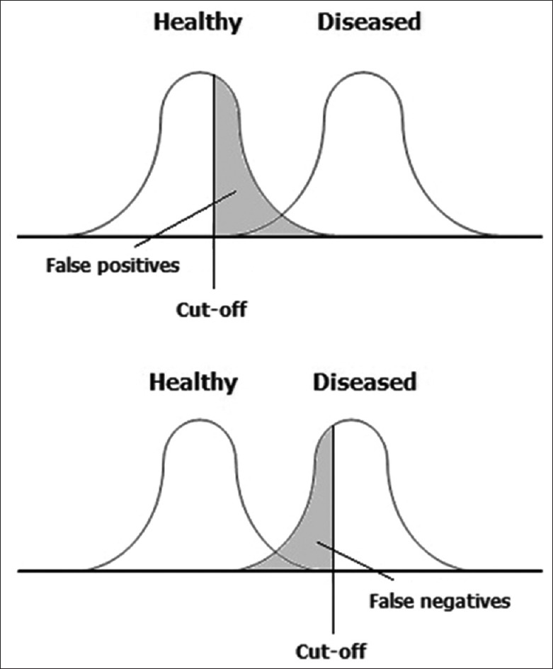
The dilemma in selection of the positivity criterion

Receiver Operating Characteristic Curve

The dilemma in the selection of cutoff value can be addressed through the receiver operating characteristic (ROC) curve which is a graphical representation of the relationship between sensitivity and specificity for a diagnostic test returning results on a numerical scale. Figure 3 depicts a ROC curve which is utilized in selecting an optimum cutoff value. This is simply a plot of the sensitivity values of a series of potential cutoffs along the Y-axis versus corresponding (1 − specificity) values along the X-axis. The (1 − specificity) value has also been called the false positive rate. At least three cutoff points, and preferably five, should be used to plot the curve. The broken line signifies no predictive ability. In general, the best cutoff point lies at or near the elbow (highest point at the left) of the curve. However, the important consideration is for the intended clinical circumstances to guide the final choice of cutoff point. If the consequences of false positives outweigh those of false negatives, then a lower point on the curve (to the left) can be chosen.

Figure 3.

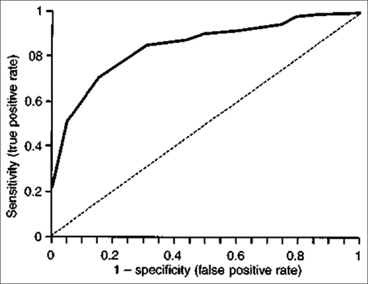
Receiver operating characteristic curve. The broken line signifies no predictive ability

An ROC curve plots the relationship between sensitivity and specificity, which are independent of prevalence; therefore, it will not be affected by changes in prevalence. The slope of the ROC curve represents the ratio of sensitivity (true positive rate) to the false positive rate. The line of equality (slope = 1.0) signifies no predictive ability. The steeper the slope, the greater the gain in PPV. The area under an ROC curve (ROC area) represents the diagnostic (or predictive) ability of the test. An ROC area of 0.5 occurs with the curve of equality (the line y = x) and signifies no predictive ability. Most good predictive scores have an ROC area of at least 0.75. Two or more predictive, or risk scores, can be compared by measuring their ROC areas.

An ROC curve may also be employed to decide on the optimum circumstances (e.g., temperature) for performing a laboratory test. The test is performed under different circumstances, and the sensitivity and specificity values obtained (in relation to a gold standard) plotted in an ROC curve. The circumstances that fall at or near the elbow of the curve are selected.

Figure 4 shows four ROC curves with different ROC areas. A perfect test (A) has an area under the ROC curve of 1. The chance diagonal (D, the line segment from 0, 0 to 1, and 1) has an area under the ROC curve of 0.5. ROC curves of tests with some ability to distinguish between those subjects with and those without a disease (Band C) lie between these two extremes. Test B with the higher area under the ROC curve has a better overall diagnostic performance than test C.

Figure 4.

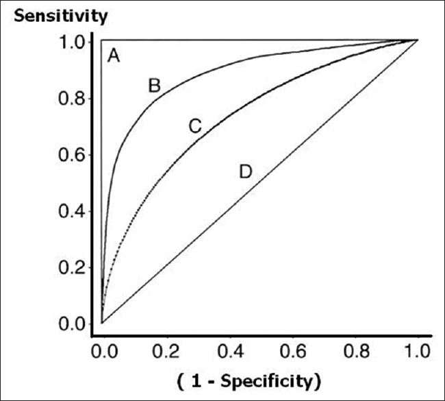
Receiver operating characteristic curves with varying area under curve

The ROC curve was first developed by electrical and radar engineers during World War II for detecting enemy objects in battlefields, which activity came within the purview of signal detection theory. In signal detection theory, an ROC curve is a graphical plot of the sensitivity versus (1 − specificity) for a binary classifier system as its discrimination threshold is varied. The name has stuck even in its application to medicine and life sciences.

Reference Range

Diagnostic test results reported as numbers are not meaningful by themselves. Their meaning comes from comparison to reference values. A reference range or reference interval denotes the “normal” range of measurements, i.e., the range to be expected if measurements are conducted repeatedly in healthy individuals. The limits of the range have been called the upper reference limit (URL) or upper limit of normal and the lower reference limit (LRL) or lower limit of normal.

Laboratory reference ranges are usually calculated from a large number of healthy volunteers, assuming a normal distribution in the population, as mean ± 1.96 standard deviations. The values of 95% of healthy individuals are then expected to fall within this range. It is acceptable that 2.5% of the time a sample value will be less than the LRL, and 2.5% of the time it will be larger than the URL.

Occasionally, only one side of the reference range is of interest, such as with tumor marker antigens, where it is generally without any clinical significance to have a value below what is usual in the population. Therefore, in such cases, only one limit of the reference range is given, and such values are rather like cutoff values or threshold values.

Alternatively, a percentile range may be adopted as the reference range. For instance, a 10^th–90^th percentile range is often taken as the reference range for anthropometric measurements. In India, these boundaries are depicted in the weight for age charts used to plot the growth of under-five children. If variation is expected to be large, the interquartile range (25^th–75^th percentile range) may be taken as the reference range. Thus, the reference price of a branded medicine in India is often expressed as the interquartile range of the prices of brands having at least 1% market share.

The use of standard score is another way of expressing numerical measurements and gauging their deviation from normality. A standard score is derived from a raw score (i.e., measured result) in a particular manner. The usual method of standardizing is to subtract the population mean from an individual raw score and then divide the difference by the population standard deviation. The resultant dimensionless quantity is popularly called the Z-score or Z-value. A positive Z-score indicates a value above the mean, while a negative score indicates value below the mean. Thus, a Z-score of – 2.5 indicates that the measured value is 2.5 times standard deviation below the mean. Note that, the Z-score is only defined if we know the population parameters; if we have only sample data for reference, then the analogous computation with sample mean and sample standard deviation yields t-score rather than Z-score. One advantage of using standard scores is to become independent of the unit of measurement that will allow comparison between different methods of measurement. Historically, bone density measurements have been expressed as Z-score, the computation of which requires reference tables showing the mean and standard deviation for the applicable race, age, gender, and skeletal site.

Agreement between Tests that Express Results in Categories - the Kappa Statistic

Jacob Cohen, in 1960, proposed the kappa (κ) statistic as a measure of inter-rater agreement on categorical variables. It is generally regarded as a more robust measure than simple percent agreement calculation since κ takes into account the agreement occurring by chance. Kappa can be used to compare the ability of different raters to classify subjects into two or more categories. Kappa can also be used to assess the agreement between alternative techniques of categorical assessment when new techniques are under study.

If the raters or tests are in complete agreement, then κ = 1. If there is no agreement among the raters or tests at all (other than what would be expected by chance), then κ = 0. The calculation of Cohen's kappa is relatively simple and can be done by hand. Use of computer software additionally allows ready estimation of the 95% CI.

As an example consider that a researcher is using USG and also CT on the same set of 273 subjects to categorize abdominal lesions as cyst, benign lump, or malignant lump. The values that he gets are as follows:

Here, the values 61, 129, and 36 are the concordant values (falling along the diagonal of concordance) and represent 82.78% agreement between the two diagnostic modalities. Kappa can be calculated as 0.711 (95% CI, 0.637–0.786), indicating fairly strong agreement between USG and CT in differentiating abdominal masses.

In general, 0≤ κ ≤1 although negative values do occur occasionally. Cohen's kappa is ideally suited for nominal (nonordered) categories. Weighted kappa can be calculated for tables with ordinal categories.

Landis and Koch (Landis JR, Koch GG. The measurement of observer agreement for categorical data. Biometrics 1977;33:159-74) suggested the following boundaries for interpreting κ values. These values, however, are arbitrary and are not accepted universally. The number of categories and subjects will affect the magnitude of the value. The kappa tends to be higher when there are fewer categories.

Interpretation of κ:

• 0.00–0.20: Poor agreement

• 0.21–0.40: Fair agreement

• 0.41–0.60: Moderate agreement

• 0.61–0.80: Substantial agreement

• 0.81–1.00: Almost perfect agreement.

Note that, Cohen's kappa measures agreement between two raters only. Fleiss’ kappa (after Joseph L. Fleiss, 1981) statistic has been used for a similar measure of agreement in categorical rating when there are more than two raters. However, Fleiss’ kappa can be used only with binary or nominal scale ratings. No version is available for ordered categorical ratings.

Financial support and sponsorship

Nil.

Conflicts of interest

There are no conflicts of interest.