SEIZURE FORECASTING AND THE PREICTAL STATE IN CANINE EPILEPSY

Abstract

The ability to predict seizures may enable patients with epilepsy to better manage their medications and activities, potentially reducing side effects and improving quality of life. Forecasting epileptic seizures remains a challenging problem, but machine learning methods using intracranial electroencephalographic (iEEG) measures have shown promise. A machine-learning-based pipeline was developed to process iEEG recordings and generate seizure warnings. Results support the ability to forecast seizures at rates greater than a Poisson random predictor for all feature sets and machine learning algorithms tested. In addition, subject-specific neurophysiological changes in multiple features are reported preceding lead seizures, providing evidence supporting the existence of a distinct and identifiable preictal state.

1. Introduction

Epilepsy affects 0.5–1% of the world’s population¹ and is characterized by recurrent, spontaneous seizures. Anti-epileptic medications are effective in many cases, but in 20–40% of cases they do not eliminate seizures². Resective surgery³ and neurostimulation^4,5 can be effective treatments if medications fail, but for many patients seizures persist despite these procedures. Further, a significant aspect of epilepsy-related disability beyond the occurrence of the seizures is their unpredictability^6–8. One consequence is that patients taking medication typically do so daily, and incur considerable side effects to prevent a condition that may happen only a few times per year^2,9,10. During initialization of treatment with anti-epileptic drugs, systemic toxicity causes treatment failure as often as lack of efficacy in controlling seizures¹¹. So, the ability to reliably forecast seizures may not only have therapeutic benefits, it might also permit patients to manage their daily activities and medications to minimize what might otherwise be a significant side-effect profile¹². In addition, a closed-loop seizure forecasting system capable of neurostimulation during preseizure warnings could abort seizures before they begin by altering the preseizure neurodynamics underlying the brain’s seizure-prone state.

Prior reports of seizure forecasting approaches follow a similar hypothesis and sequence of data processing methods^13–16: The fundamental hypothesis tested is that there exists a preictal (pre-seizure) state associated with an increased probability of seizure occurrence that can be distinguished from brain state(s) with low probability of seizure occurrence (interictal). Measurements of brain state are derived from some physiological signal (e.g., scalp EEG, intracranial (iEEG), functional MRI, or other modalities). Features are extracted from the brain state measurement to characterize the important pre-seizure changes in the underlying signals. These features are used with a labeled set of training data to create a predictive model of the brain’s state changes before a seizure event. The accuracy of the predictive model is estimated using cross validation against a portion of the labeled training data, reserved for testing¹⁷. If the accuracy estimated from cross validation is adequate, the predictive algorithm can be applied to new data, and ultimately in real time as the data is acquired¹⁸. Prior studies suggest that the characteristics and timing of the preictal brain state are subject-dependent¹⁹ and may require retraining of the predictive algorithm for every subject. Moreover, some measures of the brain state change over time²⁰. This suggests that predictive algorithms may need to be revised periodically to maintain their accuracy, and that the ability of signal-acquisition components (e.g., electrodes) to faithfully detect neurophysiologic data also changes over time.

While prior studies have demonstrated the effectiveness of machine learning methods at forecasting seizures^12,16,18,19, progress has been limited by the lack of high-quality, open-access recordings allowing direct comparison of different feature sets and algorithms²¹. In addition, the exact nature and characteristics of the changes in the iEEG signal that precede seizures remain unclear. Understanding these dynamics would assist in selection of predictive features for seizure forecasting and may provide clues to the physiological processes that generate seizures.

This study investigates the dynamics of the pre-seizure state and describes the development of a processing pipeline for seizure forecasting. Three features were evaluated for observable preictal changes and compared with the performance of cross frequency coupling reported by Alvarado-Rojas, C., et al²². The results are assessed and validated using open-access iEEG recordings from canines with naturally occurring epilepsy (see https://www.ieeg.org/ and http://msel.mayo.edu). The relative contributions of different feature sets, preprocessing methods, and predictive modeling approaches are described and assessed. The machine learning based pipeline was able to predict seizures, using a 90-minute prediction window, with an average Area Under ROC curve 0.83±0.07. The investigation on pre-seizure dynamics provided evidence supporting the existence of a distinct and identifiable preictal state.

2. Subjects and Methods

Approval of the Institutional Animal Care and Use Committee (IACUC) at Mayo Clinic, the University of Minnesota, and University of Pennsylvania were obtained for acquisition of the data analyzed in this paper.

2.1. Subjects

The NeuroVista Seizure Advisory System^23,24 was implanted in eight canine subjects with naturally occurring epilepsy and spontaneous seizures. The dogs were housed in the University of Minnesota and University of Pennsylvania veterinary clinics. The subjects were continuously monitored with video and iEEG. Anti-epileptic medications were provided as needed to the dogs during this study. Five dogs had an adequate number of seizures and length of interictal recordings for algorithm training and testing (Table 1), and data from these five dogs was used for analysis (Table 1).

Table 1.

Subjects and Seizures. The number of recorded seizures and lead (separated by 4 hours) seizures varied for each canine subject. Three canines (2, 5, and 8) had insufficient seizures and were omitted from further study.

Dog	Implanted	Recording Duration (d)	Recorded Data (d)	Annotated Seizures	Lead (4h) Seizures	Interictal Windows	Preictal Windows
1	7/30/09	476	342	47	40	166170	328
2	7/15/09	398	255	2	2
3	8/27/09	452	213	104	18	159808	345
4	5/7/12	393	298	29	27	145788	606
5	5/8/12	338	29	0	0
6	5/14/12	287	168	144	86	286	261
7	5/15/12	294	80	22	8	33649	264
8	5/16/12	290	126	0	0

2.2. Device

The NeuroVista system is pictured in Figure 1. The NeuroVista Seizure Advisory System (Figure 1) was used to acquire continuous iEEG recordings over multiple months from freely behaving canines^23,24. The system consists of (1) an Implantable Lead Assembly (ILA), (2) an Implantable Telemetry Unit (ITU); and (3) an external Personal Advisory Device (PAD), which is contained in a vest worn by the canine. The iEEG signals are recorded from the ILA contacts, filtered, amplified, and digitized (sampling rate 400 Hz) within the ITU and then wirelessly transmitted to the external PAD device. The ITU is charged daily for approximately an hour via an external inductive charging device. The PAD collected continuous iEEG data wirelessly from the ITU and stored data on removable flash media. The PAD has the capability to run embedded seizure detection algorithms, and to provide seizure warnings via a wireless data link and audible alarms²⁴, but this capability was not used in the present study.

Fig. 1.

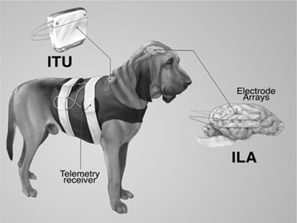
Seizure Advisory System (SAS) in Canines with Epilepsy. The implantable device for recording and storing continuous iEEG includes the Implantable Lead Assembly (ILA) consisting of four subdural electrode strips. The Implantable Telemetry Unit (ITU) is implanted beneath the dog’s shoulder and connected to the ILA. The system acquires 16 channels of iEEG and wirelessly transmits the data to the receiver.

3. Data

3.1. Acquisition

Sixteen-channel iEEG recordings sampled at 400 Hz were wirelessly transmitted to the PAD, stored on a flash memory card, and regularly uploaded to shared, central, cloud-based servers. A high sensitivity automated seizure detector was used to detect seizure-like events²⁵. Candidate iEEG detections were visually reviewed, and a synchronized recorded video was reviewed to verify and identify clinical and subclinical seizures. Intracranial EEG data from this study are freely available from Mayo Clinic (http://msel.mayo.edu/data.html) and the iEEG portal (https://www.ieeg.org/).

3.2. Data Preprocessing

Wireless telemetry between the ITU and PAD was prone to interference and short data dropouts. Data loss could also occur due to changing removable storage, battery failure in the recording device, and occasional equipment maintenance. Because of these factors, the recorded iEEG data exhibits occasional gaps, which appear as discontinuities in the recording. Figure 2 shows a recording with discontinuities and groupings of seizures. Seizures tend to occur in clusters clinically²⁶, and prediction of lead seizures is a more meaningful clinical problem. In addition, restricting analysis to lead seizures prevents postictal phenomena from contaminating the preictal iEEG data. Seizures that were not preceded by another seizure in the 4 preceding hours were considered as lead seizures. Seizures that had a recording gap greater than 5 minutes during the preceding four hours were not counted as lead seizures to allow for the possibility that the discontinuity could contain a seizure. The proportion of recorded seizures that qualified as lead seizures is listed in Table 1.

Fig. 2.

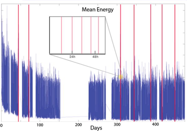
iEEG Recording with Discontinuities. Mean energy in the low frequency band illustrates occasional gaps, or discontinuities in the recorded data from device signal dropout. Seizures are marked by vertical red lines, and the expanded view shows a grouping of seizures over approximately 60 hours. Post-surgical changes in the data were noted in the first 70 days post surgery in all the recordings, and these regions were excluded from analysis.

Due to the large number of brief discontinuities, data gaps less than 20 seconds in duration were ignored and processed along with continuous data segments. Data discontinuities longer than 20 seconds were flagged, and analysis segments were chosen to avoid these gaps. The iEEG recording was classified into four categories (Figure 3) or phases: 1) the ictal period, representing recorded seizure activity of variable duration, 2) the postictal period, characterized by synchronous slow-wave activity following termination of the seizure, 3) the interictal period, which represents normal baseline activity, and 4) the preictal period, which represents a seizure-prone state, from which seizures are likely to arise. In this study we restricted the interictal iEEG periods to be a minimum of 1 week removed from marked seizures.

Fig. 3.

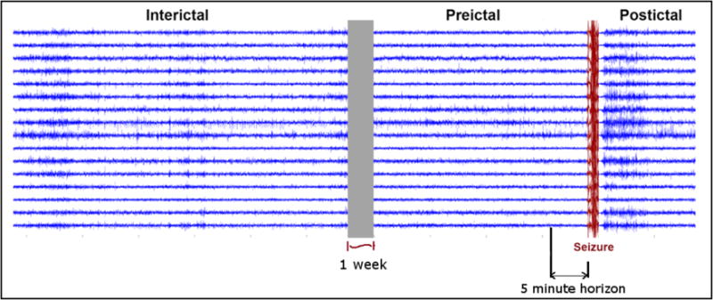
Interictal, Preictal, and Postictal Periods in Canine iEEG Recording. Interictal segments are taken at least one week prior to a seizure event. Interictal periods are treated as baseline. Preictal periods are the periods of time prior to a seizure, with a 5-minute horizon used as a test of validity. The ictal (seizure) period (marked in red) has a variable length, while the postictal period is characterized by synchronous slow-wave activity following termination of the seizure.

This very conservative standard was used to ensure the interictal training data truly represented baseline data and had the minimum possible chance of contamination with any type of pre-ictal effects. In addition, seizures occurring less than 4 hours apart from one another were excluded to minimize the potential for contamination of the preictal iEEG data by lingering subtle postictal characteristics. To ensure seizure forecasting rather than early detection of seizures and to allow for possible subtle ictal changes undetected by the expert reviewer, a 5-minute forecast horizon was used. The seizure warning had to occur at least 5 minutes before seizure onset to be counted as a valid forecast. This horizon may also enable fast-acting interventions (medications or neurostimulation) to forestall seizures in a real world application.

The raw iEEG data was transformed into derived features that may be relevant to pre-seizure activity. These features were computed on the iEEG of the interictal and preictal data for each 1-minute data window. Prior studies have shown some ability to forecast seizures using univariate spectral power in band (PIB) features^14,16, and bivariate channel synchrony measures^13,19. To analyze these classes of features, we have calculated PIB features, as well as time domain correlations (TMCO) and spectral coherence (SPCO) between different pairs of channels. The data segments were divided into non-overlapping, one-minute analysis windows. Each of these segments contained one minute of iEEG recording across all 16 recorded channels. The PIB, TMCO, and SPCO features were evaluated for each one-minute data segment.

PIB features were calculated for each channel, as power in each 1-Hz frequency band from 0–50 Hz, power in 5-Hz bands in 50–100 Hz, and power in 10-Hz bands between 100–180 Hz. The higher resolution used in calculating the powers in the lower part of the spectrum reflects the power law in EEG²⁷. Power of the signal within a frequency range [f1 – f2], P_r is obtained from Equation 3.1, where X is the Discrete Fourier Transformation (DFT) of the time domain iEEG segment.

$$P_r={\displaystyle \sum _{i=f1}^{f2}X{\left(i\right)}^2}$$ (3.1)

This produced 69 features for each channel and therefore 1104 features for a one-minute analysis window.

TMCO features were calculated as the linear absolute correlation coefficient between different pairs of channels in a one-minute clip. TMCO features were calculated for each distinct pair of the 16 channels, producing 120 TMCO features for each one-minute clip.

SPCO features were calculated as the magnitude squared coherence between different pairs of channels in a one-minute clip. The coherence function (at frequency w) of two signals x and y is given by Equation 3.4.

$$C_{xy}\left(w\right)=\frac{P_{xy}\left(w\right)}{\sqrt{P_{xx}\left(w\right)P_{yy}\left(w\right)}}$$ (3.1)

where P_xx, P_yy are power spectral densities of x, y and P_xy is the cross power spectral density of x and y. For a Fourier domain signal of N discrete frequencies, since only real frequencies are considered including DC (0Hz), a PSD of length N/2 + 1 is obtained. Since PSDs are length of N/2 + 1, spectral coherence also has a length of N/2 + 1. Magnitude squared coherences of pairs of channels at each real frequency is taken as the SPCO features.

We considered the adjacent pairs, vertical pairs, and left-right pairs (Figure 1, ILA) producing 28 pairings of electrodes. The DFT was taken with 128 points, and frequencies above the Nyquist limit were discarded, producing a 65-point spectrum and 1820 SPCO features per one-minute analysis window.

4. Prediction Algorithms

For the purpose of analyzing the iEEG data in a sequential and structured fashion, the various processing steps were incorporated into a seizure prediction pipeline with interchangeable algorithms at each step (Figure 4). The pipeline consists of four distinct steps: feature extraction, dimensionality reduction, a machine learning classifier, and forecasting and assessment. The four components are implemented modularly in MATLAB so that different techniques can be employed at each step to individually assess each component’s contribution to overall performance. The software was developed using MATLAB version 2014a and the machine learning components were implemented using MATLAB’s packages.

Fig. 4.

Predictive Pipeline Top-Level Flow Diagram. Feature Extraction from iEEG dealt with resolving Power in Band (PIB), Time Correlation (TMCO), Spectral Coherence (SPCO). Dimensionality Reduction was performed with PCA or PLS. Machine Learning Classifier analysis involved Artificial Neural Network (ANN), Support Vector Machine (SVM), and Random Forest Classifier (RFC). Forecasting was evaluated by traditional statistical means.

4.1. Feature Extraction

For each one-minute analysis window, the features PIB, TMCO and SPCO were extracted as explained in section 3. As a result, each one-minute clip had an 1104 dimensional power-in-band feature vector, a 120-dimensional time-correlation feature vector, and an 1820 dimensional spectral coherence feature vector.

4.2. Dimensionality Reduction

The dimensionality reduction (DR) block took the features extracted by the feature extraction block as input and produced a set of features with reduced dimensionality. Dimensionality reduction decreases the size of the feature set while maintaining useful information. It reduces computational time for model training, and may improve overall performance by reducing over-fitting by the ML algorithm. Two widely used DR techniques were investigated and compared to simple averaging of adjacent features, and model training without DR. Principal component analysis (PCA) is an unsupervised dimensionality reduction technique²⁸ that reduces the dimension of the data by finding orthogonal linear combinations of the original variables accounting for the largest variance in the data. Partial least squares (PLS) regression is a supervised dimensionality reduction technique that finds constituents in the feature set that contribute to the discriminability of the different classes²⁹.

In contrast to PCA, PLS regression identifies components from the features that are relevant to the different classes as linear combinations of those components. Specifically, PLS regression performs a simultaneous decomposition of the features and the classes with the requirement that the components explain the covariance between the features and the classes as much as possible. This is followed by a regression step where this decomposition is used to predict the classes.

In all trials, the dimensionality of the reduced dataset was kept constant at 50 coefficients, maintaining approximately 90% of the variance of the original data. This was kept constant over all trials to maintain a consistent comparison between techniques. For comparison the ML algorithms were also trained on the full feature set with no DR, and a set of features computed by summing every 4 adjacent features (e.g. summing every 4 frequency bins in PIB). The full PIB and SPCO feature sets overran Matlab’s memory buffers, and we trained on every 50th interictal sample. Computational time required for model training was measured for each DR method.

4.3. Machine Learning

The machine-learning block took a set of training features, corresponding labels, and a set of test features as inputs. It applied a machine learning algorithm to produce the labels and likelihood probabilities of the given test features. This block was implemented using three different ML techniques used successfully in a recent online seizure prediction competition (Brinkmann et. al., in review): Support Vector Machine³⁰ (SVM), Artificial Neural Networks³¹ (ANN) and Random Forests Classifier³² (RFC). Box constraint and misclassification costs for SVM, number of neurons, number of layers, misclassification costs for ANN, input fraction used for training, and misclassification costs for RFC were chosen by tuning on a subset of the labeled training data and achieving the best classifier performance for each subject.

4.4. Forecast Assessment

The forecast assessment block generated seizure warnings and quantified the accuracy of prediction. The seizure-forecasting algorithm generates a seizure warning when the ML algorithm’s preictal likelihood probability exceeds a defined seizure risk threshold. In the present study the seizure risk threshold was varied to create a receiver operator characteristic (ROC) curve for assessment, but in an implanted device this threshold could be tuned to optimize the balance between false positive and false negative warnings for a patient’s particular situation or preference. Once triggered, the seizure warning persisted for 90 minutes in the present study, to provide direct comparison with prior results. The total time in warning state was used as a measure of false negative rate in this study. This is a stringent measure, as a perfect seizure predictor could have up to 90 minutes of warning preceding each seizure. However this is consistent with our prior work, and it fundamentally addresses the effectiveness of a seizure-forecasting device while avoiding assumptions about sequential warnings and choice of warning duration.

The preictal state represents a period of increased seizure probability, and seizures could occur at any time during the warning period. If a seizure does not occur at some point during the warning period the warning is counted as a false positive forecast. If a seizure warning was not generated less than five minutes before a seizure, it is counted as a false negative.

Statistical significance of the seizure forecasting algorithm’s performance was evaluated against a random Poisson-process chance prediction profile, as described by Snyder et al.³³. The Poisson-process model computes p-values using identical warning duration time, warning persistence rules, and forecasting horizon as the candidate algorithm. A forecasting algorithm must perform significantly (p<0.05) better than a matched chance predictor to be considered capable of seizure forecasting. The assessment block computes several metrics, including the fraction of the lead seizures that were correctly predicted (lead sensitivity), the fraction of the total time spent in seizure warnings (time in warning), and the p-value measure for the forecasting algorithm.

The overall computational flow of the forecasting pipeline was run using a top-level wrapper (Fig. 5) that controlled which features were calculated, the dimensionality reduction method used, and the machine-learning algorithm selected, which returns the algorithm assessment. The final results are determined by a five-fold cross-validation applied with shuffling to equalize the proportion of preictal and interictal points in each cross-validation fold. Two-thirds of the one-minute windows were chosen randomly for training, while the remaining one-third were used for testing and assessment with each iteration. This produced 5 randomly overlapping training and test sets. Performance for each combination of features, dimensionality reduction, and machine learning algorithm is reported as the mean and standard deviation area under the ROC curve (AUC) for the five cross-validation folds. While sensitivity (Sn) and specificity (Sp) are practical metrics, these measures assume a specific operating point on the ROC curve. We report sensitivity at 75% specificity so as to compare the predictability at a consistent operating point, but in a real seizure forecasting device the operating point would be chosen by the patient and physician to provide the greatest possible benefit to the patient.

Fig. 5.

Seizure Forecasting Overview. The seizure forecasting workflow extracts features from the iEEG data and applies a dimensionality reduction technique to reduce the feature space for both training and testing data. For training, the labeled features are used to train a machine learning classifier, or predictor, which is used to classify the unlabeled testing data. Following classification of the testing data, performance is estimated and compared to a random predictor.

5. Results

Figure 6 shows the forecasting results using different features and analytical methods. AUC- metrics for lead seizures for each combination of techniques were averaged over all the canines to produce the means (μ) and standard errors (SE) listed in Figure 6 (A). The number of canines for which a given combination of features and methods generated a forecasting method with p<0.05, and the sensitivity of the algorithm at 75% specificity are reported in Figure 6 (B) and Figure 6 (C) respectively. The performances of the two DR techniques are compared against (i) not using any DR techniques and (ii) using a less complex DR technique (denoted as ‘SUM’ in the legends). When using PCA and PLS, the dimensionality of the features were reduced such that 95% of the variance was kept in the data. SUM method was implemented by adding adjacent k features together. The value k was chosen as 5 for PIB and 6 for SPCO. TMCO features were used as they were because of its low dimensionality.

Fig. 6.

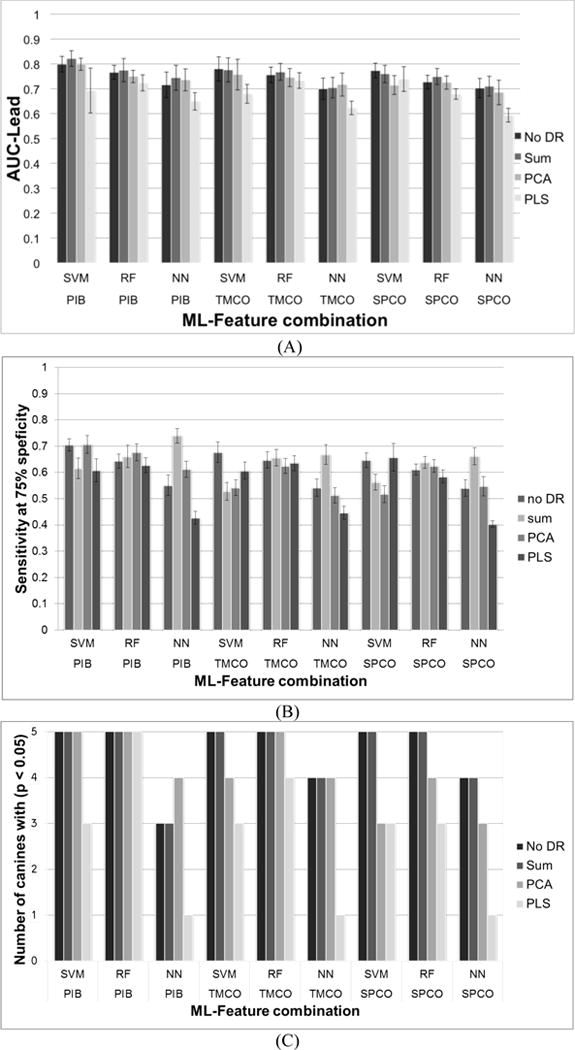
Forecasting AUC (A), Sensitivity and specificity (B), and per canine statistical significance (C) comparing the learning algorithms, features, and dimensionality reduction algorithms investigated.

Table 2 lists the measured running times for model training of each ML classifier used in the prediction framework. These running times were generated for the largest feature set (SPCO features of Subject 3) among all. The mean values and standard errors (SE) were calculated by averaging the running times over 5 cross-validations.

Table 2.

Training time of each ML classifier for different DR methods

ML	Time for model training (in seconds) – mean (SE)
	No DR	Sum	PCA	PLS
SVM	115.4 (4.2)	1132.27 (104.8)	74.8 (20.7)	1053.420 (58.6)
RFC	3.0 (0.06)	1.6 (0.3)	1.4 (0.01)	1.5 (0.05)
NN	41.9 (0.04)	22.9 (0.05)	20.2 (0.09)	18.9 (0.03)

6. Discussion

6.1. Algorithm Performance

While the SVM algorithm with PIB features had the highest mean AUC, the RF algorithm may have generalized better, achieving forecasting greater than a chance predictor in all five canines studied. The ANN learning algorithm did not perform as well as the SVM and RF algorithms in any trial, suggesting it may not be as accurate or robust as the other methods. The simple sum DR method and full feature set gave the best performance for all features and ML algorithms The DR methods reduced the feature space and algorithm training time, but in many trials PCA and PLS degraded performance somewhat.

Overall the PLS DR technique and neural network ML algorithm performed poorly compared to other techniques in many trials, suggesting these methods could be eliminated in future explorations. Good performance was obtained for all feature sets studied, suggesting preictal changes may be present and identifiable in all three feature sets.

6.2. Preictal and Postictal Data Characteristics

These results suggest that machine learning algorithms can identify subtle changes in iEEG-derived features preceding seizures. It may be possible to analyze and derive specifically what changes are occurring prior to a seizure for each subject, and this information could help us better understand the physiological changes underlying ictogenesis. Identifying the changes in the iEEG data during the transition from the interictal baseline to a preictal, seizure-permissive state is complicated by the fact that the exact timing of this transition is unknown. Prior seizure forecasting studies have analyzed data between 30 and 90 minutes preceding seizure onset. In this context, the analysis in this paper was begun 120 minutes before the seizure to ensure adequate coverage of the preictal period. Similarly, the duration of postictal effects following seizure termination is variable, and subtle effects may persist beyond visible changes in the iEEG. Two hours post seizure was also analyzed, as this extends beyond published postictal studies³⁴.

For each one-minute analysis window, PCA was applied to the 1109 PIB features, 120 TMCO features and 1820 SPCO features, and the first 10 PCs were computed for each feature group. To quantify the 10 PCs as a single numerical value, the sum of the squared (squared L2 norm) 10 PCs was calculated. The means and variances of the numerical measures were calculated considering all the lead seizure data segments for each specific subject. In addition, we reviewed cross-frequency coupling²² as a potential indicator of preictal activity. Mean power in the (30–55 Hz) and high gamma (65–100 Hz) ranges was correlated to the phase envelope of the signal in the 1–20 Hz range. The mean and variance of these correlations were plotted over the 120-minute preictal and postictal ranges. These data plots are presented for each of the five canines studied individually in Figure 6(a)–(e).

Postictal changes in the mean and variance of multiple measures were observable in most of the canine data, and the duration of these changes appeared to be specific to each canine subject. Preictal changes in the mean and variance of these metrics were observed in many of the canine subjects and preceded the seizure (where present) by 10–60 minutes. In some cases, preictal changes appeared only in the variance envelope of the metric, while the mean appeared unchanged. While this is perhaps not as instructive or practically useful for seizure forecasting as cases in which the mean value deviates (e.g., Dog 6), it does represent a change in the underlying iEEG features and may indicate the timing of a physiological preictal change. Of note, however, is that no specific feature was predictive in all dogs. This is not unexpected, as physiologic aspects of each dog’s seizure onset, seizure type, and seizure etiology are not the same. In human patients, this pathophysiologic heterogeneity would also be present, possibly to a greater extent. This fact necessitates certain engineering considerations for any future seizure-prediction device based on the paradigm presented in this report. An iterative machine learning approach would need to be used on a patient-by-patient basis and would need to use a combination of features, dimensionality reduction techniques, and machine learning paradigms that proved robust in trials such as those presented here. It would also be necessary to retrain the algorithms and reevaluate performance over time. This is because impedance changes occur at electrodes, neuroplasticity takes place, medication adjustments occur, and epileptogenic boundaries change over time.³⁵

7. Conclusions

These results demonstrate changes in multiple of iEEG features prior to seizures and support the hypothesis of a distinct, measurable, preictal (pre-seizure) state that has an increased probability of seizure occurrence. All sets of features, dimensionality reduction, and machine learning techniques investigated showed some capability to forecast seizures, but SVM and RF machine learning classifiers performed consistently better than ANN. All feature sets tested produced forecasting results greater than chance in all five canines studied with some combination of dimensionality reduction and machine learning algorithms. Preictal changes in mean and variance PIB, TMCO, and SPCO metrics as well as low gamma (30–55 Hz) and high gamma (65–100 Hz) were observed in multiple canines and occurred as early as 40 minutes before seizures (Figure 7). These results may provide insight into the timing and duration of the underlying physiological changes that lead to seizures.

Fig. 7.

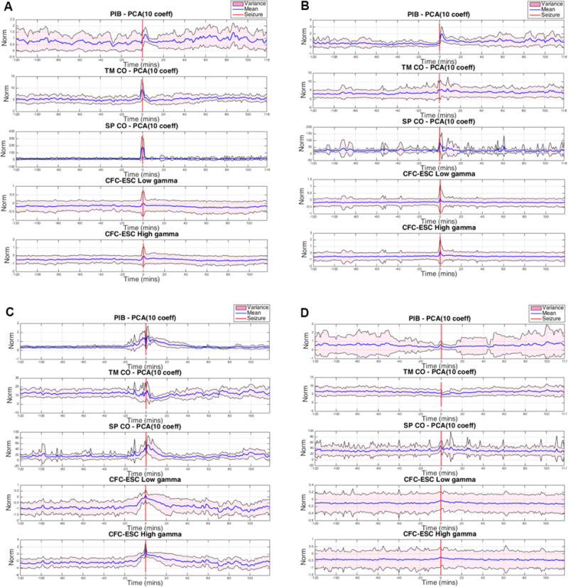
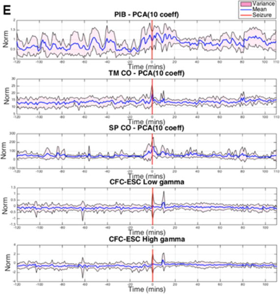
of PIB, TMCO, SPCO, and CFC Low-Gamma and High-Gamma are shown for A. Dog 1, B. Dog 3, C. Dog 4, D. Dog 6, and E. Dog 7 for two hours before and two hours after lead seizures. The red line indicates seizure onset; The mean across all seizures is plotted in blue, while the variance is shown in pink. In nearly every case, ictal changes occurred in mean and variance. Depending on the feature and dimensionality reduction combination, mean and/or variance changes occurred preictally and postictally.

References

- 1.Shorvon SD, Farmer PJ. Epilepsy in developing countries: A review of epidemiological, sociocultural, and treatment aspects. Epilepsia. 1988;29.s1:S36–S54. doi: 10.1111/j.1528-1157.1988.tb05790.x. [DOI] [PubMed] [Google Scholar]
- 2.Kwan Patrick, Brodie Martin J. Early identification of refractory epilepsy. New England Journal of Medicine. 2000;342.5:314–319. doi: 10.1056/NEJM200002033420503. [DOI] [PubMed] [Google Scholar]
- 3.Téllez-Zenteno José F, et al. Surgical outcomes in lesional and non-lesional epilepsy: A systematic review and meta-analysis. Epilepsy Research. 2010;89.2:310–318. doi: 10.1016/j.eplepsyres.2010.02.007. [DOI] [PubMed] [Google Scholar]
- 4.Fisher Robert, et al. Electrical stimulation of the anterior nucleus of thalamus for treatment of refractory epilepsy. Epilepsia. 2010;51.5:899–908. doi: 10.1111/j.1528-1167.2010.02536.x. [DOI] [PubMed] [Google Scholar]
- 5.Sun Felice T, Morrell Martha J, Wharen Robert E. Responsive cortical stimulation for the treatment of epilepsy. Neurotherapeutics. 2008;5.1:68–74. doi: 10.1016/j.nurt.2007.10.069. [DOI] [PMC free article] [PubMed] [Google Scholar]
- 6.Schulze-Bonhage Andreas, Kühn Anne. Unpredictability of seizures and the burden of epilepsy. Seizure Prediction in Epilepsy: From Basic Mechanisms to Clinical Applications. 2008 [Google Scholar]
- 7.Schulze-Bonhage Andreas, et al. Views of patients with epilepsy on seizure prediction devices. Epilepsy & Behavior. 2010;18.4:388–396. doi: 10.1016/j.yebeh.2010.05.008. [DOI] [PubMed] [Google Scholar]
- 8.Fisher Robert S. Epilepsy from the patient’s perspective: Review of results of a community-based survey. Epilepsy & Behavior. 2000;1.4:S9–S14. doi: 10.1006/ebeh.2000.0107. [DOI] [PubMed] [Google Scholar]
- 9.Kwan Patrick, Brodie Martin J. Effectiveness of first antiepileptic drug. Epilepsia. 2001;42.10:1255–1260. doi: 10.1046/j.1528-1157.2001.04501.x. [DOI] [PubMed] [Google Scholar]
- 10.Bonnett Laura J, et al. Treatment outcome after failure of a first antiepileptic drug. Neurology. 2014;83.6:552–560. doi: 10.1212/WNL.0000000000000673. [DOI] [PMC free article] [PubMed] [Google Scholar]
- 11.Cook Mark J, et al. Prediction of seizure likelihood with a long-term, implanted seizure advisory system in patients with drug-resistant epilepsy: A first-in-man study. The Lancet Neurology. 2013;12.6:563–571. doi: 10.1016/S1474-4422(13)70075-9. [DOI] [PubMed] [Google Scholar]
- 12.Schachter Steven C. Advances in the assessment of refractory epilepsy. Epilepsia. 1993;34.s5:S24–S30. doi: 10.1111/j.1528-1157.1993.tb05920.x. [DOI] [PubMed] [Google Scholar]
- 13.Andrzejak Ralph G, et al. Seizure prediction: Any better than chance? Clinical Neurophysiology. 2009;120.8:1465–1478. doi: 10.1016/j.clinph.2009.05.019. [DOI] [PubMed] [Google Scholar]
- 14.Howbert J Jeffry, et al. Forecasting seizures in dogs with naturally occurring epilepsy. PloS One. 2014;9.1:e81920. doi: 10.1371/journal.pone.0081920. [DOI] [PMC free article] [PubMed] [Google Scholar]
- 15.Mormann Florian, et al. On the predictability of epileptic seizures. Clinical Neurophysiology. 2005;116.3:569–587. doi: 10.1016/j.clinph.2004.08.025. [DOI] [PubMed] [Google Scholar]
- 16.Park Yun, et al. Seizure prediction with spectral power of EEG using cost-sensitive support vector machines. Epilepsia. 2011;52.10:1761–1770. doi: 10.1111/j.1528-1167.2011.03138.x. [DOI] [PubMed] [Google Scholar]
- 17.Bradley Andrew P. The use of the area under the ROC curve in the evaluation of machine learning algorithms. Pattern Recognition. 1997;30.7:1145–1159. [Google Scholar]
- 18.Ramgopal Sriram, et al. Seizure detection, seizure prediction, and closed-loop warning systems in epilepsy. Epilepsy & Behavior. 2014;37:291–307. doi: 10.1016/j.yebeh.2014.06.023. [DOI] [PubMed] [Google Scholar]
- 19.Brinkmann Benjamin H, et al. Forecasting seizures using intracranial EEG measures and SVM in naturally occurring canine epilepsy. PloS One. 2015;10.8 doi: 10.1371/journal.pone.0133900. [DOI] [PMC free article] [PubMed] [Google Scholar]
- 20.Wong Kin Foon Kevin, et al. Modelling non-stationary variance in EEG time series by state space GARCH model. Computers in Biology and Medicine. 2006;36.12:1327–1335. doi: 10.1016/j.compbiomed.2005.10.001. [DOI] [PubMed] [Google Scholar]
- 21.Wagenaar Joost B, et al. Neural Engineering (NER), 2013 6th International IEEE/EMBS Conference on. IEEE; 2013. A multimodal platform for cloud-based collaborative research. [Google Scholar]
- 22.Alvarado-Rojas C, et al. Slow modulations of high-frequency activity (40–140 [emsp14] Hz) discriminate preictal changes in human focal epilepsy. Scientific Reports. 2014;4 doi: 10.1038/srep04545. [DOI] [PMC free article] [PubMed] [Google Scholar]
- 23.Davis Kathryn A, et al. A novel implanted device to wirelessly record and analyze continuous intracranial canine EEG. Epilepsy Research. 2011;96.1:116–122. doi: 10.1016/j.eplepsyres.2011.05.011. [DOI] [PMC free article] [PubMed] [Google Scholar]
- 24.Coles Lisa D, et al. Feasibility study of a caregiver seizure alert system in canine epilepsy. Epilepsy Research. 2013;106.3:456–460. doi: 10.1016/j.eplepsyres.2013.06.007. [DOI] [PMC free article] [PubMed] [Google Scholar]
- 25.Gardner Andrew B, et al. One-class novelty detection for seizure analysis from intracranial EEG. The Journal of Machine Learning Research. 2006;7:1025–1044. [Google Scholar]
- 26.Haut SR. Seizure clustering. Epilepsy & Behavior. 2006;8(1):50–55. doi: 10.1016/j.yebeh.2005.08.018. [DOI] [PubMed] [Google Scholar]
- 27.Wold Svante, Esbensen Kim, Geladi Paul. Principal component analysis. Chemometrics and Intelligent Laboratory Systems. 1987;2.1:37–52. [Google Scholar]
- 28.Ferree Thomas C, Hwa Rudolph C. Power-law scaling in human EEG: relation to Fourier power spectrum. Neurocomputing. 2003;52:755–761. [Google Scholar]
- 29.Geladi Paul, Kowalski Bruce R. Partial least-squares regression: A tutorial. Analytica Chimica Acta. 1986;185:1–17. [Google Scholar]
- 30.Cortes Corinna, Vapnik Vladimir. Support-vector networks. Machine learning. 1995;20.3:273–297. [Google Scholar]
- 31.Hopfield John J. Neural networks and physical systems with emergent collective computational abilities. Proceedings of the national academy of sciences. 1982;79.8:2554–2558. doi: 10.1073/pnas.79.8.2554. [DOI] [PMC free article] [PubMed] [Google Scholar]
- 32.Breiman Leo. Random forests. Machine learning. 2001;45.1:5–32. [Google Scholar]
- 33.Snyder David E, et al. The statistics of a practical seizure warning system. Journal of Neural Engineering. 2008;5.4:392. doi: 10.1088/1741-2560/5/4/004. [DOI] [PMC free article] [PubMed] [Google Scholar]
- 34.So Norman K, Blume Warren T. The postictal EEG. Epilepsy & Behavior. 2010;19.2:121–126. doi: 10.1016/j.yebeh.2010.06.033. [DOI] [PubMed] [Google Scholar]
- 35.Dudek FE, Staley KJ. Jasper’s Basic Mechanisms of the Epilepsies. 4th. Oxford University Press; Oxford: 2012. The time course and circuit mechanisms of acquired epileptogenesis; pp. 405–415. [PubMed] [Google Scholar]