Effect of Logarithmic and Linear Frequency Scales on Parametric Modelling of Tissue Dielectric Data

Abstract

The dielectric properties of biological tissues have been studied widely over the past half-century. These properties are used in a vast array of applications, from determining the safety of wireless telecommunication devices to the design and optimisation of medical devices. The frequency-dependent dielectric properties are represented in closed-form parametric models, such as the Cole-Cole model, for use in numerical simulations which examine the interaction of electromagnetic (EM) fields with the human body. In general, the accuracy of EM simulations depends upon the accuracy of the tissue dielectric models. Typically, dielectric properties are measured using a linear frequency scale; however, use of the logarithmic scale has been suggested historically to be more biologically descriptive. Thus, the aim of this paper is to quantitatively compare the Cole-Cole fitting of broadband tissue dielectric measurements collected with both linear and logarithmic frequency scales. In this way, we can determine if appropriate choice of scale can minimise the fit error and thus reduce the overall error in simulations. Using a well-established fundamental statistical framework, the results of the fitting for both scales are quantified. It is found that commonly used performance metrics, such as the average fractional error, are unable to examine the effect of frequency scale on the fitting results due to the averaging effect that obscures large localised errors. This work demonstrates that the broadband fit for these tissues is quantitatively improved when the given data is measured with a logarithmic frequency scale rather than a linear scale, underscoring the importance of frequency scale selection in accurate wideband dielectric modelling of human tissues.

I. Introduction

The dielectric properties of biological materials have been studied widely at microwave and radio frequencies since the early 1950s [1]–[4]. These properties are of importance in both basic and applied research. The dielectric properties can be measured using numerous techniques [5]–[7]; however the open-ended coaxial probe method is most common. This method can measure the dielectric properties of biological tissues over broad frequency ranges, is non-invasive and does not require any special sample preparation [8], [9], thus enabling both in-vivo and ex-vivo measurements. The measurement procedure consists of placing the probe in contact with the sample and recording the frequency-dependent complex reflection coefficient (which is directly related to the permittivity and conductivity of the material) using a network analyser.

Computational investigation of the interaction of electromagnetic (EM) fields with biological tissues is regularly required when studying the safety of EM technologies (for example, WIFI or cell phones), and in the design of medical diagnostic or therapeutic techniques (microwave imaging, hyperthermia and ablation). Complex simulation techniques are used in order to model the effect of fields propagating in and around the body. One of the most common techniques is the finite-difference time-domain (FDTD) method [10], [11]. Other methods include, but are not limited to, the frequency-dependent FDTD (FD²DT) [12] and transmission line matrix (TLM) [13] methods. Reliable numerical simulations require accurate dielectric properties of the tissues, otherwise the results will not match well with the physical or experimental reality. In order to capture measured tissue dielectric properties in the simulations, closed form parametric models are often used. A number of parametric models have been developed; the Cole-Cole [14] model is one of the most well-known and most utilized parametric models. The Cole-Cole model is defined as:

$$\hat{\epsilon }(\omega )={\epsilon }_{\infty }+\frac{\mathrm{\Delta }{\epsilon }_c}{{(1+j\omega {\tau }_c)}^{(1-\alpha )}}+\frac{{\sigma }_s}{j\omega {\epsilon }_0}$$ (1)

where ε_∞ is the highest frequency permittivity, Δε_c is the change in the permittivity, σ_s is the static ionic conductivity, τ_c is the relaxation constant and α is an empirical parameter to broaden the dispersion. The exponent α is a positive fractional constant with a value 0 ≤ α ≤ 1, and is used to describe different spectral shapes. In general, the Cole-Cole model is used to represent wideband tissue properties in simulations. To do this, the Cole-Cole parameters must be optimised in order to obtain the best fit to the measured dielectric data.

The quality of parametric model fitting to measured data can be quantified using statistical methods. This entails examining the residuals, i.e., the errors obtained as the differences between the observed (measured) and predicted (modelled) data. The residuals can also be thought of as elements of variation unexplained by the fitted model. The general assumptions for the residuals are that they are normally and independently distributed with a mean of zero and a constant variance [15]. This implies that the model predicted values should be higher and lower than the actual data with equal probability, and the magnitude of the error should be independent of the number of data points. In other words, a high-quality fit should result in a residual distribution that is normal, whereas lower quality fits will have non-normal distributions. The normality of the distribution of a group of residuals can be assessed using one of the two most common graphical methods, a histogram or a normal probability plot. The residual analysis indicates whether the model is appropriate and the results are reasonable [15]. Different statistical tests are available to measure and validate the goodness of the curve fitting routine. The chi-squared goodness of fit, also called Pearson’s chi-squared test, is a commonly used method to describe the discrepancy between measured and predicted data points.

The quality of the fit of the data to the model can be affected by the number of poles that are used in the model. Several studies have fitted Cole-Cole models with different numbers of poles to tissue data sets over various frequency ranges. For example, Stoy et al. [16] fitted a one-pole Cole-Cole model to different mammalian tissues over the frequency range of 0.1–100 MHz. Gabriel et al. [17] formulated a four-pole Cole-Cole model for 17 different body tissues for a wide frequency range of 10 Hz–20 GHz. Lazebnik et al. [18], [19] investigated one- and two-pole Cole-Cole models over 0.5–20 GHz for healthy and malignant breast tissues. O’Rourke et al. [20] used a one-pole Cole-Cole model to fit to ex vivo normal, malignant and cirrhotic liver tissues from 0.5 to 20 GHz. More recently, Abdilla et al. [21] fit a one-pole Cole-Cole model to data from muscle and liver tissues over 0.5–40 GHz. Finally, in Sugitani et al [22], a two-pole Cole-Cole model was used to fit breast tumor, stroma and adipose tissues over 0.5–20 GHz. In general, for an optimal representation of the data, the number of poles used should correspond to the number of dielectric relaxations of the tissue over the investigated frequency range. If too small a number of poles is used than can adequately represent the dispersion regions, information will be lost. If too large a number of poles is used, then there is a risk that the Cole-Cole parameters are being fitted to noise variations and not to the data itself. Thus, selection of an appropriate number of poles is key.

Finally, there are also different ways of collecting data that may affect the quality of the fit. In this instance, we consider the effect of the frequency scale on the fitting of tissue dielectric data to Cole-Cole parametric models. In particular, we examine and quantify the difference between measurements conducted on the same tissues both with a logarithmic frequency scale and a linear frequency scale. The effect of logarithmic and linear frequency scales have never been examined quantitatively, and their impact on the quality of Cole-Cole parameter optimisation is unknown. However, in the majority of recent dielectric property studies, the linear scale is the standard choice [18], [21], [23], while logarithmic frequency spacing was mainly used in early studies [14], [16], [22], [24]–[28]. These studies have rarely provided specific justification for the selection of a linear or logarithmic frequency scale for measurements. Yet, early studies clearly state that the logarithmic frequency scale provides more evenly spaced data points around the Cole-Cole plot [14]. As a result, use of the logarithmic scale may result in fitting that is more accurate with less fit error over large frequency bands, thus resulting in more accurate dielectric models. Therefore, the aim of this paper is to examine curve fitting to the Cole-Cole model for linear and logarithmic spaced frequencies using experimental data, and to quantitatively assess whether one is superior to the other using parameter estimation metrics. To best of authors’ knowledge, this is the first and only study that quantifies the effect of logarithmic versus linear measurements on fitted dielectric data.

II. Methodology

This section describes the experimental design, the background assumptions used in the statistical analysis, and the validation tests performed.

A. Experimental Design

Two set of dielectric measurements were performed, one at the Thayer School of Engineering, Dartmouth College and the second at the National University of Ireland Galway (NUIG). At both locations, the experiments were conducted using the same dielectric probes and measurement protocol.

1) Measurements at Dartmouth

Dielectric measurements were performed on samples of bovine muscle tissue at the Thayer School of Engineering, Dartmouth College. The measurements were conducted using the commercially available slim form probe from Keysight Technologies. The 85070E dielectric probe kit was connected to the Keysight Technologies E5071B ENA series vector network analyser (VNA). The measurements were recorded at room temperature over the frequency range of 200 MHz–8.5 GHz. The selected frequency range covered the maximum frequency range of the measurement equipment. For each scale, 80 frequency points were taken. Room temperature was used as the aim of this study is to assess the linear and logarithmic scales, and these are not temperature sensitive.

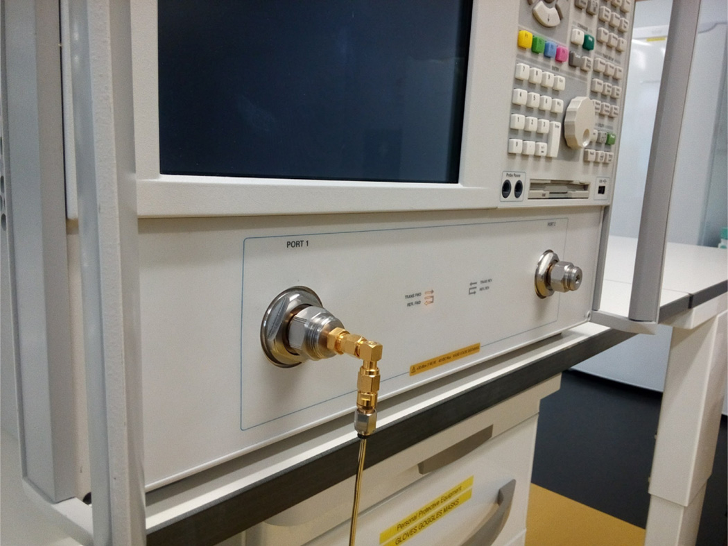
It was found through experience and multiple measurements that the cable connected to the probe is one of the main factors for uncertainty in the measurements. For this reason, in this experimental design the cable was removed and the probe was connected directly to the port of the network analyser using an N-type to SMA right angle connector, as shown in Fig. 1. The removal of the cable improved not only the stability and repeatability of the measurements, but also removed the measurement sagging effect and the requirement to regularly refresh the calibration during repeated measurements.

Fig. 1.

Photograph of the slim form probe connection with the network analyser.

The VNA was calibrated using the common open/short/load calibration mechanism. The Smith chart was visually inspected to ensure a proper short for the calibration. Deionised water was used as the load in the calibration process. All calibrations were validated with standard reference materials before conducting measurements. The measurements were performed on the same tissue sample with both linear and logarithmic frequency scales. The sample was placed in good contact with the probe and five measurements at five different points were recorded with the same number of sample points for each scale.

2) Measurements at NUIG

The second set of dielectric measurements was performed at the National University of Ireland Galway, with a broader frequency range and a selection of tissue types. Measurements were conducted on bovine muscle, bovine fat, ovine liver and ovine kidney tissues. The Keysight Technologies slim form probe from the 85070E dielectric probe kit was used and was connected to the Agilent Technologies E8362B ENA series vector network analyser (VNA). The measurements were recorded at room temperature over the larger frequency range of 200 MHz–20 GHz using 80 frequency points for each scale. The experimental protocol, calibration, and measurement conditions were matched to those of the experiment at Dartmouth. The probe was connected directly to the port of the VNA using an N-type to SMA right angle connector, without the need for a cable. The sample was placed in good contact with the probe and five measurements at each point were recorded for five different points on each sample using logarithmic and linear scales. The five measurements at each point were averaged to form one measurement.

The tissue samples for both sets of experiments were obtained from an abattoir. Standard handling procedures were followed to ensure the samples were not contaminated. Handling was consistent across all samples and measurements. All measurements on a given sample were performed within 30 minutes to avoid the tissue drying effect. To examine the uncertainty in the measurement system, measurements were performed on standard reference materials. In particular, 15 measurements were performed over three calibrations of the network analyser on the reference material 0.1 M NaCl (saline) at 22°C. These measurements were used to calculate the total combined uncertainty (TCU) as in [29]. The errors were calculated for each measured parameter separately. The TCU was found to be = 2.1 for the relative permittivity, and = 3.4 for the conductivity. For the relative permittivity, the repeatability is within 2.1% and the accuracy is within 0.26%. For the conductivity, the repeatability in the measurement is within 2.3% and the accuracy is within 4.2%. The same measurements were also conducted on ethanol (at 19.1°C), in order to validate measurements of lower permittivity materials. In this case, the total uncertainty was found to be less than 3.5%, across all frequencies. Note that no drift or cable movements were included in this uncertainty analysis as there was no cable in place during the measurements, and the measurements were always performed immediately following calibration thus drift was negligible.

3) Data Processing

Once the measurements were completed, the Cole-Cole model was used to fit the measured data. As discussed in the Introduction, the Cole-Cole model is selected because it is one of the most commonly used parametric model in well known dielectric studies. According to the literature [17], [30], each dispersion region is the manifestation of a polarization mechanism characterized by a single relaxation frequency. This implies that one pole is sufficient to characterize one dispersion region. Thus, the number of poles to be used in the Cole-Cole model of the data is typically based on the number of relaxations within the frequency range of interest. Within our frequency range, two relaxations exist [3], [31], [32]; thus, the two-pole Cole-Cole model is an appropriate choice. However, one-pole Cole-Cole model was also fitted to our data in order to compare the results with literature where the simplified one-pole Cole-Cole has been commonly used.

Accordingly, one-pole and two-pole Cole-Cole models were separately fitted to the measured data using a genetic algorithm (GA) [33] for both frequency scales. The choice of GA over the traditional least square method (LSM) is based on the fact that the GA does not require an initial estimation. The values of the parameters Δε, σ_s, ε_∞ and τ were allowed to vary within the GA. The values of these parameters typically differ by many orders of magnitude. To overcome this problem, logarithmic values of parameters were used rather than their linear values. The cost function C_GA minimized by the GA is given below:

$$C_{GA}=\sum _{i=1}^N[{\mathit{\text{log}}}_{10}{(m_r({\omega }_i)-c_r({\omega }_i)]}^2+{[{\mathit{\text{log}}}_{10}(m_i({\omega }_i)-c_i({\omega }_i))]}^2$$ (2)

The function is the sum of the squared differences between the measured data and the multi-pole Cole-Cole model. m_r(ω_i) and m_i(ω_i) are the real and the imaginary parts of the measured data, respectively; and c_r(ω_i) and c_i(ω_i) are the real and the imaginary parts of the Cole-Cole function, respectively. The population size for the GA was 1000 individuals. The tournament selection method was used with parameter value of 20. The mutation probability and crossover fraction were set to 0.1 and 0.9, respectively.

Bound value ranges were applied to each of the parameters in order to ensure that the GA did not converge towards local optima. The bound values, shown in Table I, were selected in accordance with the literature [34]. The fitted curves and the measured data were then used to calculate the residuals as the fractional errors. The residuals were calculated for the real and imaginary parts of the complex permittivity and then combined to form a set of total residuals for each fitted curve.

TABLE I.

Bound value ranges for the parameters of GA

Parameter	Value range
ε∞	1–50
Δε	1–100
σs	0.0001 – 1
τ	1 µs – 10 ps

B. Background Assumptions

A statistical analysis is based on a set of assumptions. These assumptions relate to the characteristics of the data under analysis. If these assumptions are not met then the results can be misleading or erroneous. In particular, and key to this study, the validity of these assumptions determines the goodness of a fitted model. The background assumptions for residual analysis are as follows [15]:

1. The data is of a single category;

2. The residuals are normally distributed (the residuals are equally distributed around the mean forming a bell-shaped curve);

3. The residuals have zero mean;

4. The residuals are independent (the behaviour of the residuals is not affected by changes in the frequency range or the sample size);

5. The residuals are random (the model is predicting values higher and lower than the actual values with equal probability);

6. The residuals have constant variance.

C. Assumption Validation Tests

In order to quantitatively assess the fitting results using the linear and logarithmic scale data, different statistical tests have been applied to the calculated residuals. The validation of the above-mentioned assumptions by the statistical test quantifies the goodness of the fitting results. In other words, a high-quality fit will have residuals that meet the requirements specified by all of the noted assumptions.

The normality of the residuals was first visualised by obtaining the histogram of each set of residuals. The overall pattern of the residuals should be similar to the bell-shaped pattern for normal distribution. The histogram provided an initial visual validation for the distribution of the residuals. For a more accurate judgement of the residuals distribution, a normality test was applied. The test sorted the residuals into ascending order and then calculated the cumulative probability of each residual:

$$P(i_{\mathit{\text{th}}}\mathit{\text{residual}})=\frac{i}{(N+1)}$$ (3)

where P denotes the cumulative probability, i is the order of the residual and N is the total number of residuals. The calculated p-values are then used to obtain the normal probability plot (also known as a Q-Q plot). An approximate straight line in the plot confirms that the residuals are independent and normally distributed.

Once it is confirmed that the residuals satisfy the above mentioned conditions, the chi-squared goodness-of-fit test is used to quantitatively examine the quality of the fit by measuring how well the predicted data corresponds to the measured data. In particular, the chi-squared test, also referred to as χ² test, estimates the probability of the residuals under the assumption of no association (also known as the “null hypothesis”) [15]. Low probability values reject the null hypothesis and validate that the fitted curve is close to the measured data. The test is defined as:

$${\chi }^2=\sum _{i=1}^n\frac{{(O_i-E_i)}^2}{E_i}$$ (4)

where O_i is the observed or calculated data, E_i is the expected or actual measured data, and n is total number of data points.

III. Results

In the first subsection, the fitting results of the two-pole Cole-Cole model are presented and discussed. The second subsection describes the statistical analysis of residuals obtained from the two-pole Cole-Cole model fitting. The third subsection compares the results of using single-pole versus two-pole for both the linear and logarithmic spacing.

A. Fitting Results

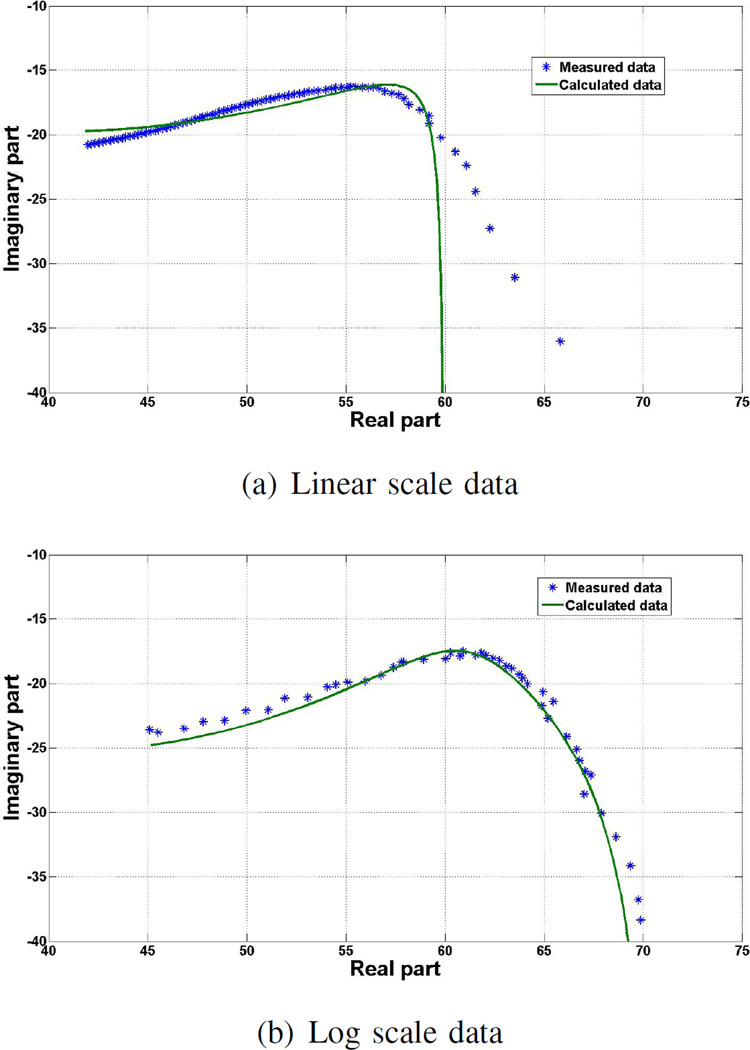
Fig. 2 shows the Cole-Cole plots for one of the five measurements performed at Dartmouth using linear and logarithmic scales.

Fig. 2.

Cole-Cole plots of a) linear and b) log scale data: model shown with the measured data points using bovine muscle tissue over the frequency range of 200 MHz–8.5 GHz.

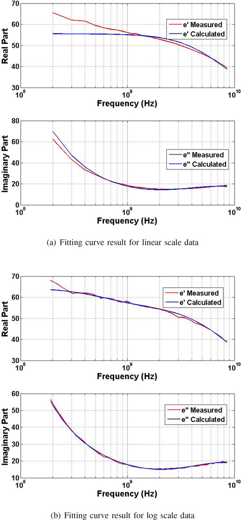
As expected, Fig. 2 shows that the points in the Cole-Cole plots are more evenly spaced for measurements with the logarithmic scale as compared to measurements with the linear scale [14]. The linear scale only has a few data points at the lower frequencies, while most of the data points are grouped at higher frequencies. Using the logarithmic scale, the points are evenly distributed over the entire frequency range. An uneven distribution of data points with the linear scale will result in poor fitting results at the lower frequencies, as can be seen in Fig. 3. There is a significant difference between the measured and modelled data up to about 1 GHz when using linear frequency scale. Further, with the logarithmic scale, the points are well distributed over the relaxation frequency where the shape of the curve is changing most rapidly and the difference between the modelled and measured data is smaller than with linear scale.

Fig. 3.

Cole-Cole model fitting results of the complex permittivity for: a) linear and b) log scale data.

The poor fitting at the lower frequencies as a result of uneven spacing in the linear scale may not be observed if the overall average error of the fitted curve is used as a performance metric, because the large number of points at higher frequencies (where the error is low) will “average out” the larger errors at low frequencies. Furthermore, the different number of data points around each relaxation do not lead to a proper representation of the measurement behaviour.

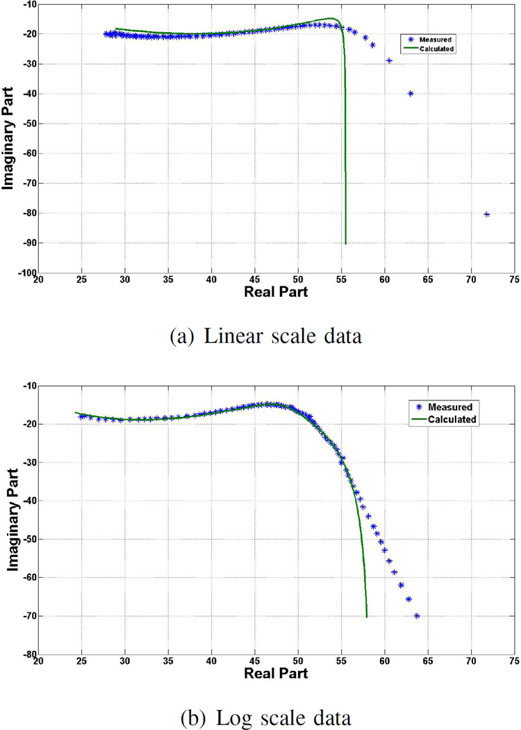
Similar results can be seen Fig. 4, which shows a sample Cole-Cole plot for one of the five measurements performed on ovine kidney tissue at NUIG. Although the fitting at the lower frequencies is not perfect with logarithmic scale data, this fitting is still observably superior to that of the linear scale data. Furthermore, the difference between the measured and model data across the relaxation frequency using the logarithmic scale is again smaller than with linear scale. At higher frequencies, the curve is well behaved in both cases due to the fact that the change in dielectric properties at high frequencies is quite small as compared to at low frequencies.

Fig. 4.

Cole-Cole plots of a) linear and b) log scale data: model shown with the measured data points using ovine kidney tissue over the frequency range of 200 MHz–20 GHz.

B. Statistical Analysis

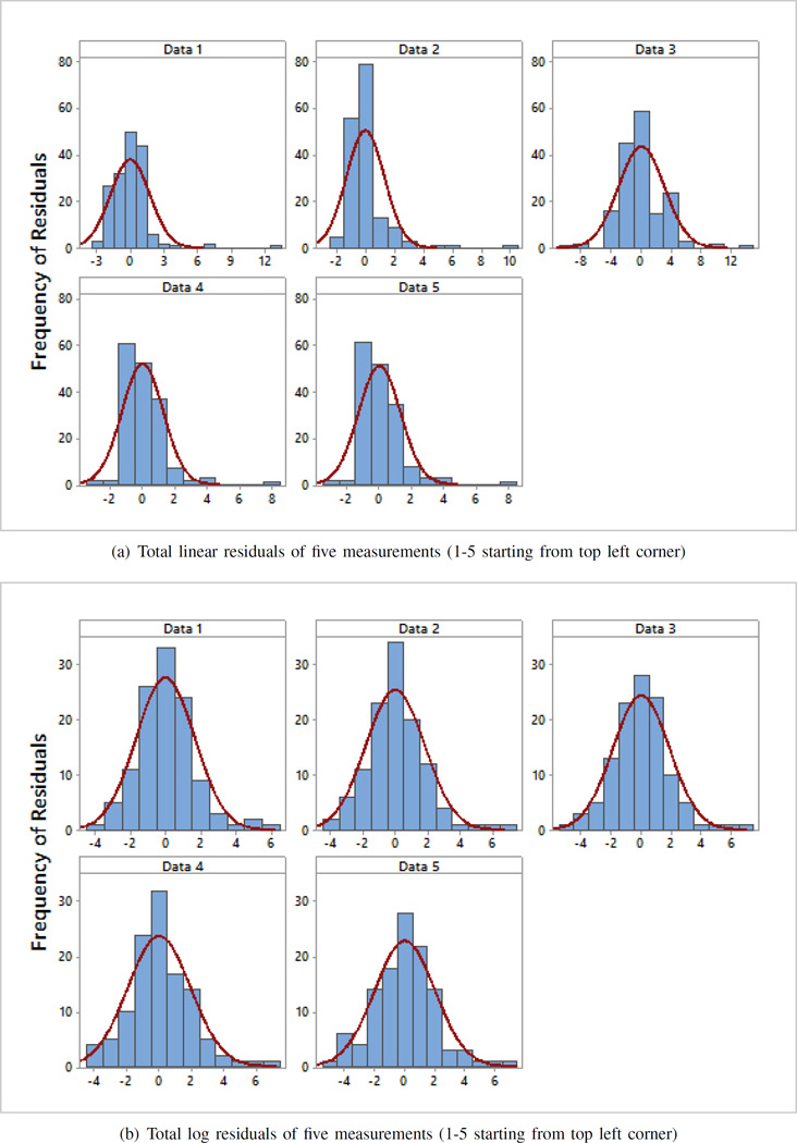
Histograms of the residuals of the fit to the Cole-Cole model are presented in Fig. 5 for all measurements performed at Dartmouth using both linear and logarithmic scales.

Fig. 5.

Histograms of residuals for five measurements using a) linear and b) log scale. The red envelope is the distribution curve in each plot. These results demonstrate that the residuals from the log scale measurements are more normally distributed than the residuals from the linear scale measurements. This indicate that the error in logarithmic case is random and independent.

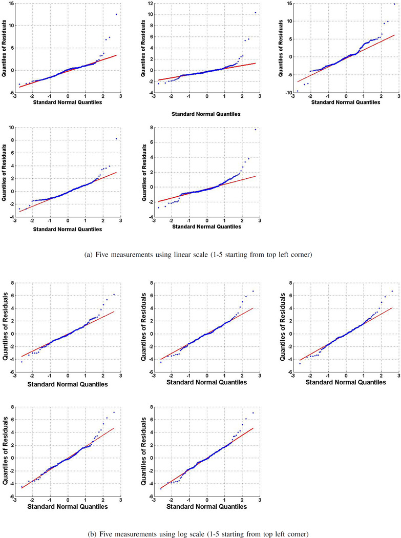
The histograms show that the residuals for logarithmic scale are more normally distributed around the mean than the residuals for linear scale. The histograms also show that in almost all cases, logarithmic residuals are in the range of −4 to 6, whereas, the ranges for linear residuals vary. The histograms visually validate the normality of residuals, but in order to quantify the normality, the Kolmogorov-Smirnov normality test [15] is applied on all residual sets. The resultant Q-Q plots are shown in Fig. 6. The p-values for all five sets of linear residuals are less than 0.05, rejecting the null hypothesis that the data is normally distributed. In the case of logarithmic residuals, the p-values for all five sets are more than 0.05, thus the residuals are normally distributed.

Fig. 6.

Q-Q plots of residuals for five measurements using a) linear and b) log frequency scales. These plots demonstrate that the residuals from the log scale measurements are normally distributed; whereas the residuals from the linear scale measurements are not. This suggests that the error in logarithmic case is random and independent.

Next, the chi-squared goodness of fit test is applied to the residuals and the resultant values are presented in Table II. The chi-squared values for the logarithmic scale data are in the range of 3 to 12 for all measurements. For linear scale measurements, the chi-squared values are higher, ranging from 8 to 55. The large chi-squared values indicate poor data fitting to the model.

TABLE II.

Chi-squared values for linear and log scale fitting results using two-pole Cole-Cole (200 MHz–8.5GHz)

(a) Linear scale
Linear Scale	Chi-squared Value
Data 1	34.06
Data 2	55.34
Data 3	8.48
Data 4	24.80
Data 5	23.06

(b) Log scale
Log Scale	Chi-squared Value
Data 1	4.78
Data 2	11.69
Data 3	3.53
Data 4	4.85
Data 5	5.55

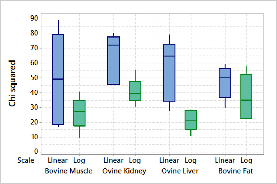
Similar results are obtained from the dielectric measurements at NUIG. In all cases, the normality tests have demonstrated that the logarithmic scale residuals are more normally distributed compared to the linear scale residuals except the results of bovine fat where the choice of scale has no significant impact on the fitting results. The reason for this is that fat has the lowest permittivity values and the change in the permittivity over frequency is small relative to the other tissues. The chi-squared test values for the measurements performed at NUIG are summarized in Fig. 7.

Fig. 7.

Box plot of chi-squared values for log and linear measured data of bovine muscle, ovine kidney, ovine liver and bovine fat tissues over the frequency range of 200 MHz–20 GHz using the two-pole Cole-Cole model.

For all tissues, the median chi-squared value across measurements is lower (implying better fit) for logarithmic data than for linear data. Further, the highest (worst) chi-squared values for each tissue also come from the linear data. These results suggest that the quality of the fit is generally better with logarithmic scale measurements than with linear scale measurements, for this broadband test scenario.

C. Comparison with One-pole Cole-Cole

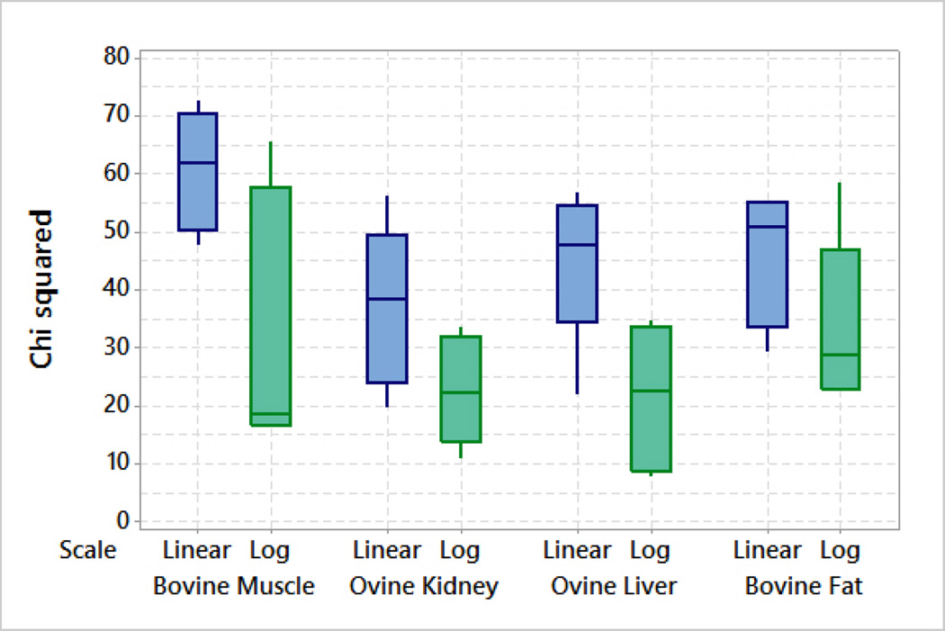
As many studies have used one-pole Cole-Cole model, the one-pole Cole-Cole model is also fitted to the measured dielectric data for completeness. The chi-squared test is then applied to quantify the goodness of fit obtained for all measurements with both frequency scales. The resulting chi-squared test values for the measurements performed at Dartmouth are presented in Table III and for the measurements performed at NUIG are summarized in the box plot in Fig. 8. For all tissues, the median chi-squared values are lower with the logarithmic scale data. Thus, the logarithmic scale consistently provides a better fit than the linear scale for these data sets.

TABLE III.

Chi-squared values for linear and logarithmic scale fitting results using the one-pole Cole-Cole model (200 MHz–8.5GHz)

(a) Linear scale
Linear Scale	Chi-squared Value
Data 1	18.57
Data 2	21.66
Data 3	15.92
Data 4	28.33
Data 5	35.36

(b) Log scale
Log Scale	Chi-squared Value
Data 1	16.82
Data 2	14.09
Data 3	17.39
Data 4	9.42
Data 5	14.82

Fig. 8.

Box plot of chi-squared values for bovine muscle, ovine kidney, ovine liver and bovine fat tissues over the frequency range of 200 MHz–20 GHz using one pole Cole-Cole model.

IV. Conclusions

In this paper, dielectric measurements were performed on bovine muscle, bovine fat, ovine kidney and ovine liver tissues using both linear and logarithmic frequency scales. The measured data was analysed to quantitatively assess the effects of frequency spacing on parametric model fitting of the measured data. The analysis has shown that the logarithmic scale distributes the frequency points in such a way that there are more points in the frequency regions where the largest changes in dielectric properties occur (i.e. around the relaxation points). This distribution of points results in more accurate modelling of the measured data, especially at low frequencies. While it has been known that a logarithmic frequency scale provides a more even distribution of measurement data on a Cole-Cole plot than linear frequency scale [14], use of the log scale has not been regularly incorporated into modern research studies of wideband tissue properties. The results of this work demonstrate that the residuals produced using logarithmic scale are more normally distributed than the linear scale residuals, and the chi-squared values demonstrate that the goodness of fit to logarithmic scale data is better than the fitting to linear scale data. This is the first and only study that quantitatively assesses the effect of logarithmic and linear measurements on the fitted dielectric data.

In general, the choice of scale depends on the experimental requirements. If only a narrow frequency band is used in the measurement, the linear scale may produce a high quality fit. Further, if the overall average error is more important that the quality of the fit, the linear scale may be used even with wideband measurements as it will produce less average error than the logarithmic scale due to the large number of data points at high frequencies that have lower error than the data points at low frequencies. However, if the broadband quality of the fitted curve is important, then logarithmic scale can provide better fitting results. Significantly, a better quality fit results in less error both in dielectric models, and in the EM simulations that they are used in. Moreover, the choice of performance metrics also depends on the experimental requirements. The use of a well established statistical framework not only summarises the overall error of the fitted curve but also quantitatively evaluates the quality of the fitted curve. This work has conclusively shown that the measurements taken in logarithmic scale represent the dielectric properties more accurately than the measurements taken in linear scale for a variety of tissues, when the frequency range is wide, and when it includes more than one relaxation.

References

- 1.England T. Dielectric properties of the human body for wavelengths in the 1–10 cm range. Nature. 1950;16:480–481. doi: 10.1038/166480b0. [DOI] [PubMed] [Google Scholar]
- 2.Cook HF. The dielectric behaviour of some types of human tissues at microwave frequencies. British Journal of Applied Physics. 1951;2(10):295. [Google Scholar]
- 3.Schwan HP. Electrical properties of tissue and cell suspensions. Advances Biological and Medical Physics. 1957;5:147–209. doi: 10.1016/b978-1-4832-3111-2.50008-0. [DOI] [PubMed] [Google Scholar]
- 4.Peyman A, Gabriel C, Grant EH, Vermeeren G, Martens L. Variation of the dielectric properties of tissues with age: the effect on the values of SAR in children when exposed to walkie-talkie devices. Physics in medicine and biology. 2009;54(2):227–241. doi: 10.1088/0031-9155/54/2/004. [Online]. Available: http://www.ncbi.nlm.nih.gov/pubmed/19088390. [DOI] [PubMed] [Google Scholar]
- 5.Westphal WB. Dielectric Materials and Applications, AR von Hippel. New York: Wiley; 1954. Dielectric measuring techniques; pp. 63–122. [Google Scholar]
- 6.Bussey HE. Measurement of RF Properties of Materials A Survey. Proceedings of the IEEE. 1967;55(6):1046–1053. [Google Scholar]
- 7.Afsar MN, Birch JR, Clarke R, Chantry G. The Measurement of the Properties of Materials. Proceedings of the IEEE. 1986;74(1):183–199. [Google Scholar]
- 8.Marsland T, Evans S. Dielectric measurements with an open-ended coaxial probe. IEE Proceedings H-Microwaves, Antennas and Propagation. 1987;134(4):341. [Google Scholar]
- 9.Athey TW, Stuchly MA, Stuchly SS. Measurement of radio frequency permittivity of biological tissues with an open-ended coaxial line: Part I. IEEE Transactions on Microwave Theory and Techniques. 1982;30(1):82–86. [Google Scholar]
- 10.Young JL. Propagation in Linear Dispersive Media: Finite Difference Time-Domain Methodologies. 1995;43(4):422–426. [Google Scholar]
- 11.Kelley DF, Luebbers RJ. Piecewise linear recursive convolution for dispersive media using FDTD. IEEE Transactions on Antennas and Propagation. 1996;44(6):792–797. [Google Scholar]
- 12.Feliziani M. FD2TD Analysis of Electromagnetic Field Propagation in Multiploe Debye Media With and Without Convolution. Progress In Electromagnetics Research B. 2012;42(July):181–205. [Google Scholar]
- 13.Russer P, Russer JA. Application of the Transmission Line Matrix (TLM) method to EMC problems. Asia-Pacific Symposium on Electromagnetic Compatibility, APEMC 2012 - Proceedings. 2012:141–144. [Google Scholar]
- 14.Cole KS, Cole RH. Dispersion and Absorption in Dielectrics I. Alternating Current Characteristics. The Journal of Chemical Physics. 1941;9(4):341. [Google Scholar]
- 15.Hines WW. Probability and Statistics in Engineering and Management Science. Vol. 3 John Wiley and Sons; 1999. [Google Scholar]
- 16.Stoy RD, Foster KR, Schwan HP. Dielectric properties of mammalian tissues from 0.1 to 100 MHz: a summary of recent data. Physics in medicine and biology. 1982;27:501–513. doi: 10.1088/0031-9155/27/4/002. [DOI] [PubMed] [Google Scholar]
- 17.Gabriel S, Gabriel C, Lau RW. The dielectric properties of biological tissues: III. Parametric models for the dielectric spectrum of tissues. Physics in medicine and biology. 1996;41(11):2271–2293. doi: 10.1088/0031-9155/41/11/003. [DOI] [PubMed] [Google Scholar]
- 18.Lazebnik M, Popovic D, McCartney L, Watkins CB, Lindstrom MJ, Harter J, Sewall S, Ogilvie T, Magliocco A, Breslin TM, Temple W, Mew D, Booske JH, Okoniewski M, Hagness SC. A large-scale study of the ultrawideband microwave dielectric properties of normal, benign and malignant breast tissues obtained from cancer surgeries. Physics in medicine and biology. 2007 Oct;52(20):6093–6115. doi: 10.1088/0031-9155/52/20/002. [DOI] [PubMed] [Google Scholar]
- 19.Lazebnik M, McCartney L, Popovic D, Watkins CB, Lindstrom MJ, Harter J, Sewall S, Magliocco A, Booske JH, Okoniewski M, Hagness SC. A large-scale study of the ultrawideband microwave dielectric properties of normal breast tissue obtained from reduction surgeries. Physics in medicine and biology. 2007;52(10):2637–2656. doi: 10.1088/0031-9155/52/10/001. [DOI] [PubMed] [Google Scholar]
- 20.O’Rourke AP, Lazebnik M, Bertram JM, Converse MC, Hagness SC, Webster JG, Mahvi DM. Dielectric properties of human normal, malignant and cirrhotic liver tissue: in vivo and ex vivo measurements from 0.5 to 20 GHz using a precision open-ended coaxial probe. Physics in medicine and biology. 2007;52(15):4707–4719. doi: 10.1088/0031-9155/52/15/022. [Online]. Available: http://www.ncbi.nlm.nih.gov/pubmed/17634659. [DOI] [PubMed] [Google Scholar]
- 21.Abdilla L, Sammut C, Mangion L. Dielectric properties of muscle and liver from 500 MHz–40 GHz. Electromagnetic Biology and Medicine. 2013;32(2):244–252. doi: 10.3109/15368378.2013.776436. [DOI] [PubMed] [Google Scholar]
- 22.Sugitani T, Kubota SI, Kuroki SI, Sogo K, Arihiro K, Okada M, Kadoya T, Hide M, Oda M, Kikkawa T. Complex permittivities of breast tumor tissues obtained from cancer surgeries. Applied Physics Letters. 2014;104(25):253 702. (1–5) [Google Scholar]
- 23.Lazebnik M, Converse M, Booske JH, Hagness SC. Ultrawideband temperature-dependent dielectric properties of animal liver tissue in the microwave frequency range. Physics in medicine and biology. 2006;51(7):1941–1955. doi: 10.1088/0031-9155/51/7/022. [DOI] [PubMed] [Google Scholar]
- 24.Davidson DW, Cole RH. Dielectric Relaxation in Glycerol, Propylene Glycol, and n-Propanol. The Journal of Chemical Physics. 1951;19(12):1484. [Google Scholar]
- 25.Schwan HP, Foster KR. RF Field Interactions with Biological Systems: Electrical Properties and Biopphysical Mechanisms. Proceedings of the IEEE. 1980;68(1):104–113. [Google Scholar]
- 26.Surowiec A, Stuchly SS, Eidus L, Swarup A. In vitro dielectric properties of human tissues at radiofrequencies. Physics in medicine and biology. 1987;32(5):615. doi: 10.1088/0031-9155/32/5/007. [DOI] [PubMed] [Google Scholar]
- 27.Dias CJ. Determination of a distribution of relaxation frequencies using a combination of time and frequency dielectric spectroscopies. IEEE Conference on Electrical Insulation and Dielectric Phenomena. 1997;2(5):475–478. [Google Scholar]
- 28.Kun S, Peura RA. The influence of measurement frequencies on the accuracy of tissue impedance parametric modeling. Proceedings of the First Joint BMES/EMBS Conference. 1999;2:820. [Google Scholar]
- 29.Gabriel C, Peyman A. Dielectric measurement: error analysis and assessment of uncertainty. Phys. Med. Biol. 2006;51(23):6033–6046. doi: 10.1088/0031-9155/51/23/006. [DOI] [PubMed] [Google Scholar]
- 30.Grant PEH, Ph D, P F. Biological effects of microwaves and radio waves. 1981;128(9):8–12. [Google Scholar]
- 31.Foster KR, Schepps JL, Schwan HP. Microwave dielectric relaxation in muscle. a second look. Biophysical journal. 1980;29(2):271. doi: 10.1016/S0006-3495(80)85131-9. [DOI] [PMC free article] [PubMed] [Google Scholar]
- 32.Schwan H. Electrical properties of tissues and cell suspensions: mechanisms and models; Proceedings of 16th Annual International Conference of the IEEE Engineering in Medicine and Biology Society; 1994. pp. 70–71. [Google Scholar]
- 33.Clegg J, Robinson MP. A genetic algorithm for optimizing multipole Debye models of tissue dielectric properties. Physics in Medicine and Biology. 2012;57:6227–6243. doi: 10.1088/0031-9155/57/19/6227. [DOI] [PubMed] [Google Scholar]
- 34.Gabriel S, Gabriel C, Lau RW. The dielectric properties of biological tissues: II. Measurements in the frequency range 10 Hz to 20 GHz. Physics in medicine and biology. 1996;41(11):2251–2269. doi: 10.1088/0031-9155/41/11/002. [DOI] [PubMed] [Google Scholar]