Bounded-observation Kalman Filtering of Correlation in Multivariate Neural Recordings

Abstract

A persistent question in multivariate neural signal processing is how best to characterize the statistical association between brain regions known as functional connectivity. Of the many metrics available for determining such association, the standard Pearson correlation coefficient (i.e., the zero-lag cross-correlation) remains widely used, particularly in neuroimaging. Generally, the cross-correlation is computed over an entire trial or recording session, with the assumption of within-trial stationarity. Increasingly, however, the length and complexity of neural data requires characterizing transient effects and/or non-stationarity in the temporal evolution of the correlation. That is, to estimate dynamics in the association between brain regions. Here, we present a simple, data-driven Kalman filter-based approach to tracking correlation dynamics. The filter explicitly accounts for the bounded nature of correlation measurements through the inclusion of a Fisher transform in the measurement equation. An output linearization facilitates a straightforward implementation of the standard recursive filter equations, including admittance of covariance identification via an autoregressive least squares method. We demonstrate the efficacy and utility of the approach in an example of multivariate neural functional magnetic resonance imaging data.

I. INTRODUCTION

In neural signal processing, functional connectivity refers to the characterization of statistical association between brain regions [1]. Several spectrotemporal metrics may be used to determine this association. Functional connectivity intends to describe the extent to which disparate brain regions exhibit synchronized activity. It may, or may not, correspond to anatomical connections [2]. The outcome of any application of functional connectivity analysis amounts to a weighted graph, where the recorded regions are the nodes and the statistical associations constitute the edge weights. For electrophysiological recordings, increasing effort has been directed at elucidating these weights in a directed fashion (see e.g., [3], [4] and the references therein). Despite these advances, the Pearson correlation coefficient – the simple, zero-lag correlation between time series – remains a familiar, reliable and widely used association metric, particularly in neuroimaging [5].

The Pearson correlation (hereafter referred to as the cross-correlation) is usually obtained over a single trial. Implicit in this use is stationarity of the underlying data. When trials are long, such an assumption is problematic. For instance, a ‘medium’ correlation value (e.g., 0.5), may arise between regions that are consistently associated across the trial, or, between regions that alternate between strong and weak association. In order to disambiguate these scenarios, one requires a way to track correlations on a finer time scale. Computing correlations on shorter sub-trial windows (i.e., binning) can provide such resolution at the expense of increased noise susceptibility. In this note, we propose a simple Kalman-filter based method to estimate the underlying dynamic evolution of correlation structure. The filter operates on the time series constructed by computing correlations in successive bins. We note that, while similar approaches have been developed for this purpose [6], they do not constrain the observation (i.e., the cross-correlation). As a consequence, the resulting estimate may lie outside of the limits [−1, 1]. In the formulation presented herein, we assume that each successive correlation arises from a standard autoregressive model, transformed through a Fisher transform (a normalizing nonlinearity that constrains the random walk between [−1, 1]). The Fisher transform is commonly used for performing correlation statistical significance testing [7].

Due to the nature of the nonlinearity, the problem reduces to a straightforward Kalman approach after an inversion step. We proceed by presenting the filter equations and demonstrating their efficacy in tracking dynamic correlations in synthetic networks. We show that the covariance matrices needed for implementation can be successfully obtained in a data driven way through the use of an autoregressive least squares method (ARLS). Finally, we demonstrate proof-of-concept by applying the method to an example of a high-dimensional neural data obtained via functional magnetic resonance imaging (fMRI). The overall method can be used as a front-end for dimensionality reduction methods for the purposes of classification and/or denoising.

The remainder of this note is organized as follows. In Section II we formulate the model and filter. In Section III we provide the relevant equations and provide simulation results, including use of ARLS. The example involving multivariate fMRI recordings is presented in Section III-D. Conclusions and Future work are discussed in Section IV.

II. MODEL FORMULATION

A. Dynamic Correlation Model

Let z_k, k = 1, 2, … be a vector time series of correlation values between pairs of brain regions. We assume that z_k arises from an underlying state x_k ∈ ℝ^N via

$${\mathbf{z}}_k={\mathbf{F}}^{-1}({\mathbf{x}}_k),$$ (1)

where the function F⁻¹ is vector-valued inverse Fisher transform which can be written as

$${\mathbf{F}}^{-1}\left(\right[\begin{array}{c}\hfill x^1\hfill \\ \hfill ⋮\hfill \\ \hfill x^N\hfill \end{array}\left]\right)=\left[\begin{array}{c}\hfill \text{tan}\mathrm{h}(x^1)\hfill \\ \hfill ⋮\hfill \\ \hfill \text{tan}\mathrm{h}(x^N)\hfill \end{array}\right].$$ (2)

Such a function bounds the state within [−1, 1] and is the standard transformation of the cross-correlation into a normally distributed variable[7]. We assume that x_k obeys a standard, linear state space model of the form

$${\mathbf{x}}_k={\mathbf{A}}_k{\mathbf{x}}_{k-1}+{\mathbf{w}}_{k-1},$$ (3)

$${\mathbf{y}}_k={\mathbf{F}}^{-1}({\mathbf{C}}_{\mathbf{k}}{\mathbf{x}}_k+{\mathbf{v}}_k).$$

Here, the state noise process w_k ∈ ℝ^N is an N-dimensional random vector with multivariate Gaussian distribution having zero mean and covariance matrix Q_w ∈ ℝ^{N × N}, the noise vector v_k ∈ ℝ^N is a zero-mean multivariate Gaussian random vector with covariance matrix R_v ∈ ℝ^{N × N}. Bounded nature of correlation coefficients result in a non-Gaussian noise for the observation vector y_k. The covariance Q_w determines the extent to which correlation can change in successive measurements, while R_v simply characterizes measurement noise. In this sense, the vector y_k consists of noisy observations of pairwise correlation values. We assume that state noise and measurement noise are uncorrelated.

We seek the optimal filter for obtaining the state estimate ẑ_k in the sense of minimum mean-squared error (MMSE), i.e.,

$$\underset{{\mathbf{ẑ}}_k}{\text{min }}𝔼\left[{\Vert {\mathbf{ẑ}}_{\mathbf{k}}-{\mathbf{z}}_{\mathbf{k}}\Vert }_2^2\right].$$ (4)

Central to this problem is the calculation of the probability density function (p.d.f.) of the state vector at any given time k, conditioned on 𝒴_k = {y₀, y₁, …, y_k}, the set of all the past observations. The presence of the nonlinearity (2) complicates this calculation, but only slightly since F is smooth and invertible. Thus, it follows immediately that we can obtain a surrogate measurement

$${\mathbf{d}}_k=\mathbf{F}({\mathbf{y}}_k),$$ (5)

such that d_k is linear in the state x_k. Note that (1) directly yields the p.d.f. of z_k from that of x_k. Thus, the problem (4) reduces to the classical Kalman filter to obtain the (Gaussian) p.d.f. of x_k given 𝒴_k [8], [9], based on the measurements d_k.

III. RESULTS

A. Filter Equations

It follows directly from (3)–(5) that the p.d.f. p(y_k|x_k) can be written as

$$p({\mathbf{y}}_k|{\mathbf{x}}_k)=\frac{1}{|{\mathbf{J}}_k|}p({\mathbf{v}}_k=\mathbf{F}({\mathbf{y}}_k)-{\mathbf{C}}_{\mathbf{k}}{\mathbf{x}}_k),$$ (6)

where p (v_k = F(y_k) − C_kx_k) is p.d.f. of v_k, a zero-mean multivariate Gaussian with covariance matrix R_v. A standard Bayesian approach thus yields the posterior density p (x_k|𝒴_k), which is Gaussian with covariance matrix (Σ) and mean (μ) as

$$\mathbf{\Sigma }={({{\mathbf{P}}_{\mathbf{k}|\mathbf{k}-\mathbf{1}}}^{-1}+{{\mathbf{C}}_{\mathbf{k}}}^T{{\mathbf{R}}_{\mathbf{v}}}^{-1}{\mathbf{C}}_{\mathbf{k}})}^{-1},$$ (7)

$$\mu =\mathbf{\Sigma }\times ({{\mathbf{P}}_{\mathbf{k}|\mathbf{k}-\mathbf{1}}}^{-\mathbf{1}}{\hat{\mathbf{x}}}_{\mathbf{k}|\mathbf{k}-\mathbf{1}}+{{\mathbf{C}}_{\mathbf{k}}}^{\mathbf{T}}{{\mathbf{R}}_{\mathbf{v}}}^{-\mathbf{1}}\mathbf{F}({\mathbf{y}}_{\mathbf{k}})).$$

The Kalman update equations are thus

$${\hat{\mathbf{x}}}_{k|k-1}={\mathbf{A}}_k{\hat{\mathbf{x}}}_{k-1|k-1},$$

$${\mathbf{P}}_{\mathbf{k}|\mathbf{k}-\mathbf{1}}={\mathbf{A}}_k{\mathbf{P}}_{\mathbf{k}-\mathbf{1}|\mathbf{k}-\mathbf{1}}{\mathbf{A}}_k^T+{\mathbf{Q}}_{\mathbf{w}},$$

$${\hat{\mathbf{x}}}_{k|k}={({{\mathbf{P}}_{\mathbf{k}|\mathbf{k}-\mathbf{1}}}^{-1}+{{\mathbf{C}}_{\mathbf{k}}}^T{{\mathbf{R}}_{\mathbf{v}}}^{-1}{\mathbf{C}}_{\mathbf{k}})}^{-1}\times ({{\mathbf{P}}_{\mathbf{k}|\mathbf{k}-\mathbf{1}}}^{-1}{\hat{\mathbf{x}}}_{k|k-1}+{{\mathbf{C}}_{\mathbf{k}}}^T{{\mathbf{R}}_{\mathbf{v}}}^{-1}\mathbf{F}({\mathbf{y}}_k)),$$ (8)

$${\mathbf{P}}_{\mathbf{k}|\mathbf{k}}={({{\mathbf{P}}_{\mathbf{k}|\mathbf{k}-\mathbf{1}}}^{-1}+{{\mathbf{C}}_{\mathbf{k}}}^T{{\mathbf{R}}_{\mathbf{v}}}^{-1}{\mathbf{C}}_{\mathbf{k}})}^{-1}.$$

In the subsequent results, we assume an initial multivariate Gaussian prior x_0|−1 with mean x̂_0|−1 and covariance of P_0|−1. We note that, for the problem (4), (8) returns the optimal estimate. After obtaining state estimate x̂_k|k, the correlation coefficients ẑ_k are approximated as ẑ_k = F⁻¹(x̂_k|k).

B. Example: Simulation

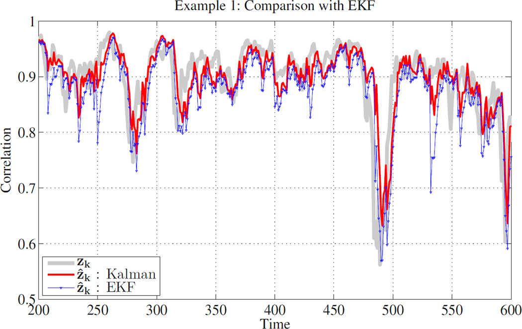
To illustrate the proposed filter, we simulate a univariate example of the system (3) with A = C = 1, Q_w = 0.1 and R_υ = 0.05. Fig. 1 shows the estimate of the correlation, i.e., z_k, using the proposed filter, as well as the results of naive application of the Extended Kalman Filter (EKF) based on linearization of (2) [10], [11]. Clearly, state estimation using proposed optimal filter is closest to the true state of the system. This result is expected because EKF is simply a linearization of F⁻¹(), which will produce poor results when the argument of the function is large (i.e., large correlation values).

Fig. 1.

Example 1: Estimation of the state in system (3) with A = C = 1, Q_w = 0.1 and R_υ = 0.05 using optimal non-linear filter for bounded observation (red) and naive application of EKF (blue).

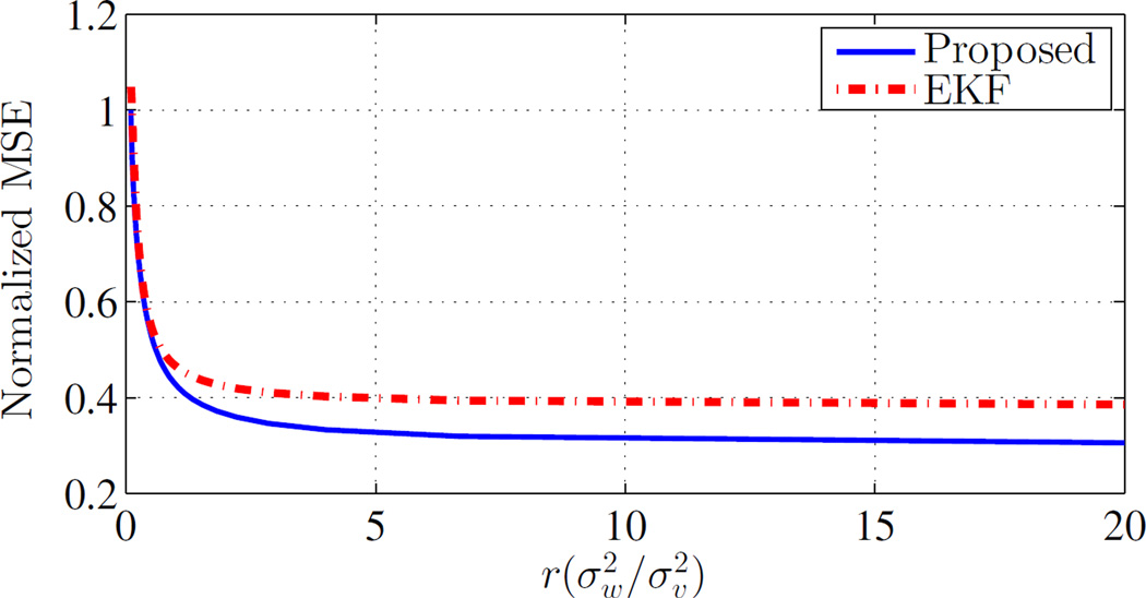
Fig. 2 illustrates mean-square error (MSE) for the proposed optimal filtering compared to EKF for different noise parameter values. In this simulation, a 4-dimensional system with A = C = I₄ is considered. The process and measurement noise are considered in the form of ${\mathbf{Q}}_{\mathbf{w}}={\sigma }_{\mathbf{w}}^{\mathbf{2}}{\mathbf{I}}_{\mathbf{4}}$, ${\mathbf{R}}_{\mathbf{v}}={\sigma }_{\mathbf{v}}^{\mathbf{2}}{\mathbf{I}}_{\mathbf{4}}$ and each time MSE is calculated for a specific ratio of $r={\sigma }_{\mathbf{w}}^2/{\sigma }_{\mathbf{v}}^2$. It can be seen in this figure that by increasing r, MSE is decreased for both filters. Also, It can be seen that optimal filter always has better performance in term of MSE compare to EKF.

Fig. 2. Normalized MSE versus the ratio of process and measurement noise.

Here, $r={\sigma }_{\mathbf{w}}^2/{\sigma }_{\mathbf{v}}^2$ with A = C = I₄, ${\mathbf{Q}}_{\mathbf{w}}={\sigma }_{\mathbf{w}}^{\mathbf{2}}{\mathbf{I}}_{\mathbf{4}}$ and ${\mathbf{R}}_{\mathbf{v}}={\sigma }_{\mathbf{v}}^{\mathbf{2}}{\mathbf{I}}_{\mathbf{4}}$.

C. Covariance Estimation

The most significant obstacle in implementation of filters of the form (8) is selection of the covariance matrices Q_w and R_v. Here, we use the popular autoregressive least squares (ARLS)[12]–[14] method to compute, in a data-driven fashion, estimates of our filter covariances. In ARLS, a prior value is assigned for each of the covariances and the innovations of the subsequent filter is used to update the estimates of Q_w and R_v in the next iteration. More explicitly, assuming the the model (3) is time-invariant, we obtain an filtered estimate of the observations with non-exact covariance matrices. By computing the innovations and steady-state distributions, the problem of estimating Q_w and R_v then becomes a one-step least-squares optimization problem. In our case, the ALS solution is again facilitated by using the output linearized measurement (5).

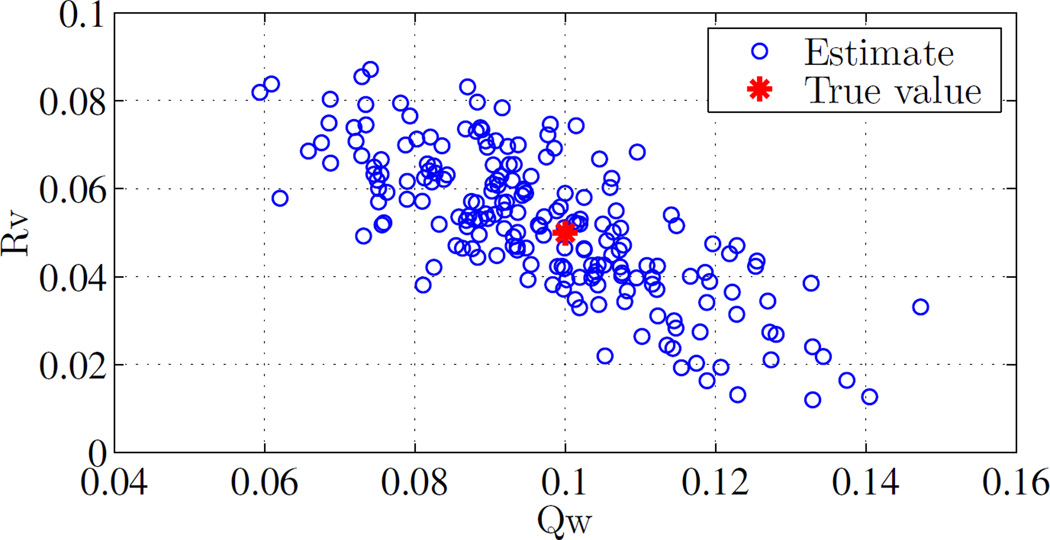
Figure 3 shows the outcome of ALS when applied in a Monte Carlo (n = 200) fashion to the system described above. It is clear that the estimate covariances are in agreement of the true values.

Fig. 3.

Estimation of Q_w and R_υ using auto-regressive least squares. Outcome of n = 200 Monte Carlo trials is shown, demonstrating concentration around the true value. System is as specified in the example of Section III-B.

D. Application to Multivariate Functional Magnetic Resonance Imaging (fMRI)

The Kalman-filtering approach outlined above is particularly useful under the assumption of edge independence, i.e., the matrix A in (3) is the identity matrix. In this case, the n–dimensional update problem decomposes into n 1-dimensional problems, alleviating computational issues related to high-dimensionality. In brain imaging applications involving large numbers of recording sites, this yield a highly practical front-end correlation estimator.

To demonstrate the utility of the method, we apply it to an example of neural recordings obtained via fMRI in human volunteers¹. For this particular dataset, we concatenated trials to create a single long recording. The concatenation creates known time-points at which the temporal structure of the correlation would be expected to change. This particular dataset contains 160 brain regions, yielding 12720 correlation pairs. We bin the data over 5 datapoints (sampling rate of 0.45Hz), yielding an effective correlation window of around 10 seconds. We note, however, that the final result is largely insensitive to bin size.

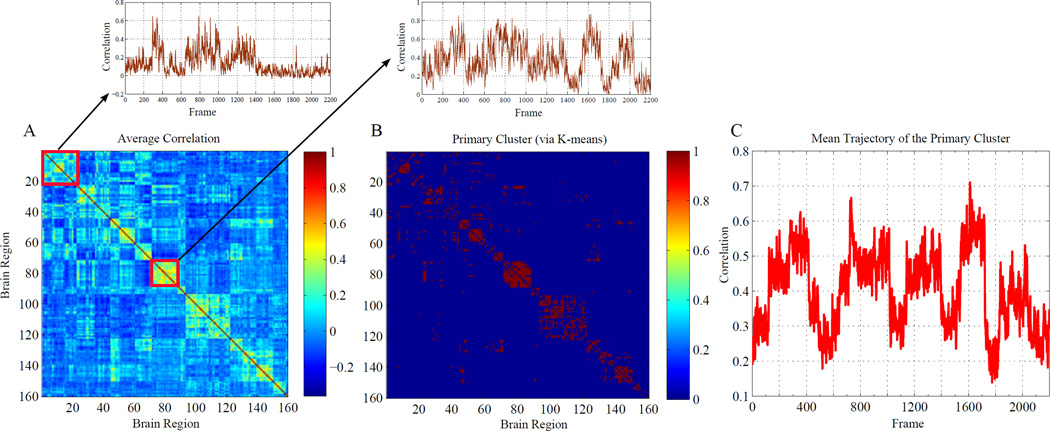
Figure 4 illustrates how the method can yield particular insight into the temporal evolution of correlation structure. In Figure 4A, the average correlation map, calculated over the entire recording, is shown. This map highlights clear regions of interest that exhibit seemingly significant correlation structure. What this static map cannot discern is the extent to which these correlations may be changing over the course of the recording. By applying the ARLS-parametrized filter (8) to the data, we can obtain estimates of the correlation trajectories. These trajectories can be subsequently processed with any flavor of clustering or dimensionality reduction technique. In our case, we use the standard unsupervised clustering algorithm k–means [20]. A Bayesian information criterion (BIC) is used to determine the number of clusters returned by the k-means procedure [21]. A salient cluster of edges emerges that closely matches the high-correlation edges in the static map (Fig. 4B). Figure 4C plots the average trajectory of this cluster, where it is clearly seen that regions of ‘high’ correlation in the static map actually consist of epochs of very correlated activity, interspersed by epochs that are more weakly correlated. As noted above, in the case of this example, this temporal structure is expected as a consequence of the data concatenation described above. In this sense, the result demonstrates the capacity of the method to deliver meaningful spatiotemporal structure, even in the case of high dimensional data.

Fig. 4. Disambiguating correlation dynamics.

(A) Static pairwise correlation for n = 160 channels of fMRI recordings. This ‘recording’ actually consisted of several concatenated datasets, thus creating artificial nonstationarity. Regions of interest are indicated by warmer colors. Application of the filtering procedure yields the temporal trajectory associated with each static correlation pair. The average of these trajectories over two regions of interest (indicated by red squares) are shown. (B) In total, we obtain 12720 pairwise correlation trajectories. Use of the standard clustering technique k-means yields a primary salient region of interest that closely matches the ‘warm’ regions in (A) (red indicates membership). (C) The mean of all trajectories represented in (B), illustrating the (expected) nonstationarity underlying the static characterization in (A).

IV. DISCUSSION & FUTURE WORK

This note presents a bounded-observation Kalman filter for estimating correlation dynamics in neural recordings. The metric of interest – the Pearson correlation coefficient – is constrained to [−1, 1], necessitating the inclusion of a Fisher transform in the filter equations. Inversion of data to create a surrogate measurement facilitates straightforward derivation of the recursive filter equations and data-driven parametrization via the autoregressive least squares technique.

Under assumptions of independence, the consequent solution can be tractably obtained, even in the case of high dimensional data. We apply it to an example of fMRI data, showing that it can yield meaningful trajectories. We note that the results are relatively insensitive to the size of the sub-windows used to obtain the correlation time series. In future work, we will explore more principled ways of determining this window size. We note, unsurprisingly, that in the absence of filtering, the raw time series are exceedingly noisy and difficult to visualize.

The method outlined here can serve as an efficient front-end to downstream classification algorithms for extracting salient spatiotemporal dynamics and/or rejecting artifacts and noise. In future work, we plan to deploy the method in this capacity in a more systematic study of correlation dynamics in several neuroimaging recording modalities.

REFERENCES

- 1.Sporns O, Tononi G, Edelman GM. Connectivity and complexity: the relationship between neuroanatomy and brain dynamics. Neural Networks. 2000;13(8–9):909–922. doi: 10.1016/s0893-6080(00)00053-8. [DOI] [PubMed] [Google Scholar]
- 2.Damoiseaux JS, Greicius MD. Greater than the sum of its parts: a review of studies combining structural connectivity and resting-state functional connectivity. Brain Struct. Funct. 2009;213(6):525–533. doi: 10.1007/s00429-009-0208-6. [DOI] [PubMed] [Google Scholar]
- 3.Kamiński M, Ding M, Truccolo WA, Bressler SL. Evaluating causal relations in neural systems: Granger causality, directed transfer function and statistical assessment of significance. Biological Cybernetics. 2001;85(2):145–157. doi: 10.1007/s004220000235. [DOI] [PubMed] [Google Scholar]
- 4.Friston KJ, Harrison L, Penny W. Dynamic causal modelling. NeuroImage. 2003;19(4):1273–1302. doi: 10.1016/s1053-8119(03)00202-7. [DOI] [PubMed] [Google Scholar]
- 5.Van Dijk KR, Sabuncu MR, Buckner RL. The influence of head motion on intrinsic functional connectivity MRI. NeuroImage. 2012;59(1):431–438. doi: 10.1016/j.neuroimage.2011.07.044. [DOI] [PMC free article] [PubMed] [Google Scholar]
- 6.Kang J, Wang L, Yan C, Wang J, Liang X, He Y. Characterizing dynamic functional connectivity in the resting brain using variable parameter regression and kalman filtering approaches. Neuroimage. 2011;56(3):1222–1234. doi: 10.1016/j.neuroimage.2011.03.033. [DOI] [PubMed] [Google Scholar]
- 7.Hotelling H. New light on the correlation coefficient and its transforms. J. R. Statist. Soc. B. 1953;15(2):193–232. [Google Scholar]
- 8.Kalman RE. A new approach to linear filtering and prediction problems. J. Basic Eng. 1960;82(1):35–45. [Google Scholar]
- 9.Kalman RE. Contributions to the theory of optimal control. Bol. Soc. Mat. Mexicana. 1960;5(2):102–119. [Google Scholar]
- 10.Chen Z. Bayesian filtering: From kalman filters to particle filters, and beyond. Statistics. 2003;182(1):1–69. [Google Scholar]
- 11.Einicke GA. Smoothing, filtering and prediction-estimating the past, present and future. New York: InTech; 2012. [Google Scholar]
- 12.Odelson BJ, Rajamani MR, Rawlings JB. A new autocovariance least-squares method for estimating noise covariances. Automatica. 2006;42(2):303–308. [Google Scholar]
- 13.Åkesson BM, Jørgensen JB, Poulsen NK, Jørgensen SB. A tool for kalman filter tuning. Comput.-Aided Chem. Eng. 2007;24:859–864. [Google Scholar]
- 14.Åkesson BM, Jørgensen JB, Poulsen NK, Jørgensen SB. A generalized autocovariance least-squares method for kalman filter tuning. J. Process Control. 2008;18(7):769–779. [Google Scholar]
- 15.Fox MD, Zhang D, Snyder AZ, Raichle ME. The global signal and observed anticorrelated resting state brain networks. J. Neurophysiol. 2009;101(6):3270–3283. doi: 10.1152/jn.90777.2008. [DOI] [PMC free article] [PubMed] [Google Scholar]
- 16.Power JD, Mitra A, Laumann TO, Snyder AZ, Schlaggar BL, Petersen SE. Methods to detect, characterize, and remove motion artifact in resting state fMRI. NeuroImage. 2014;84:320–341. doi: 10.1016/j.neuroimage.2013.08.048. [DOI] [PMC free article] [PubMed] [Google Scholar]
- 17.Smyser CD, Snyder AZ, Neil JJ. Functional connectivity MRI in infants: exploration of the functional organization of the developing brain. NeuroImage. 2011;56(3):1437–1452. doi: 10.1016/j.neuroimage.2011.02.073. [DOI] [PMC free article] [PubMed] [Google Scholar]
- 18.Power JD, Cohen AL, Nelson SM, Wig GS, Barnes KA, Church JA, Vogel AC, Laumann TO, Miezin FM, Schlaggar BL, et al. Functional network organization of the human brain. Neuron. 2011;72(4):665–678. doi: 10.1016/j.neuron.2011.09.006. [DOI] [PMC free article] [PubMed] [Google Scholar]
- 19.Raichle ME. The restless brain. Brain Connectivity. 2011;1(1):3–12. doi: 10.1089/brain.2011.0019. [DOI] [PMC free article] [PubMed] [Google Scholar]
- 20.Hartigan J. Clustering Algorithms, ser. Wiley Series in Probability and Mathematical Statistics. New York: 1975. [Google Scholar]
- 21.Goutte C, Hansen LK, Liptrot MG, Rostrup E. Feature-space clustering for fMRI meta-analysis. Human brain mapping. 2001;13(3):165–183. doi: 10.1002/hbm.1031. [DOI] [PMC free article] [PubMed] [Google Scholar]