Determining protein similarity by comparing hydrophobic core structure

Abstract

Formal assessment of structural similarity is − next to protein structure prediction − arguably the most important unsolved problem in proteomics. In this paper we propose a similarity criterion based on commonalities between the proteins’ hydrophobic cores. The hydrophobic core emerges as a result of conformational changes through which each residue reaches its intended position in the protein body. A quantitative criterion based on this phenomenon has been proposed in the framework of the CASP challenge. The structure of the hydrophobic core − including the placement and scope of any deviations from the idealized model − may indirectly point to areas of importance from the point of view of the protein’s biological function. Our analysis focuses on an arbitrarily selected target from the CASP11 challenge. The proposed measure, while compliant with CASP criteria (70–80% correlation), involves certain adjustments which acknowledge the presence of factors other than simple spatial arrangement of solids.

1. Introduction

The CASP (Critical Assessment of protein Structure Prediction) project was launched in 1994, originally as a global forum dedicated to prediction of protein structures on the basis of amino acid residue sequences. The goal of the project is to coordinate global efforts leading to improvements in protein structure prediction. The project maintains a set of known (although confidential and accessible only to members of the organizing committee) protein sequences, which are periodically made available to participants via e-mail. Results comprising evaluation statistics along with evaluation of individual targets are published on the project portal at [1].

Each participant is tasked with predicting the conformation of the input polypeptide chain (i.e. determine the spatial coordinates of each of its constituent atoms). The project operates in a biannual cycle, giving participants time to invent and develop structure prediction algorithms.

The CASP jury assesses the similarity of the models (structures proposed by project participants) and the target structures (determined using experimental means). All similarity metrics are based on geometric classification of the proposed system. Differences in the placement of each atom enable determination of prediction accuracy [2]. Progressive evolution of similarity metrics can be tracked by reviewing introductory publications which accompany each edition of CASP [3, 4, 5, 6, 7, 8, 9, 10, 11, 12, 13, 14, 15, 16, 17, 18, 19, 20, 21, 22, 23, 24, 25, 26].

Following superimposition of model and target folds, the distances between the positions of individual atoms serve as input for model accuracy assessment. This step involves various metrics which measure local as well as global similarity. Consequently, an important part of the CASP challenge is to validate the similarity assessment methods themselves.

While the predicted conformation of selected fragments may be perfectly accurate, these fragments may nevertheless be misaligned with the remainder of the molecule [27]. In such cases − as mentioned above − special algorithms are applied to assess local and global similarity. No universal similarity assessment algorithm exists − instead, many competing algorithms are proposed, each suited to a range of potential applications.

As already indicated, CASP is also interested in new algorithms and methods of comparing models with targets. This work proposes a method based on the similarity of hydrophobic cores in input structures. Our approach appears promising for the following reasons:

• 1.It supports a holistic assessment of the protein molecule since the hydrophobic core is an emergent property which depends on the spatial location of all residues.
• 2.It hints upon the location of biologically active sites within the protein body.
• 3.It acknowledges the influence of the aqueous environment, which is a critical aspect in protein folding studies. The fuzzy oil drop (FOD) model, which will be explained in the next section, can be used to predict various properties of the target protein, such as its solubility.

The novelty of applying the fuzzy oil drop model in the presented study hinges upon the fact that − rather than focusing on pair-wise interactions between individual atoms − our approach enables global assessment of the protein structure, factoring in the contribution of all residues to the emergent hydrophobic core.

The focus of our analysis is an arbitrarily selected target from the CASP11 challenge. Results of assessment using different methods published online [28] have been compared with the analysis of the hydrophobic core structure in the model structures submitted by participants. Our analysis focuses on publicly available models recognized as optimal by each team taking part in the project (labeled “_1”). Comparative analysis indicates generally good agreement of the FOD-based assessment results with the official metrics applied by CASP. In some cases, however, differing results have been obtained. Our goal is therefore to explain the reason for these differences. The structure of the hydrophobic core in native proteins seems to acknowledge aim-oriented deviations from the idealized hydrophobicity distribution as expressed by the fuzzy oil drop model. These local deviations very frequently correlate with the biological activity of the target protein.

2. Materials and methods

2.1. Structure prediction accuracy methods applied in the CASP project

Throughout its 20-year history CASP has proposed many methods to formally express the similarity between the “model” (predicted conformation) and the “target” (actual conformation as revealed by X-ray crystallography or NMR spectroscopy). The most basic method, focused on the geometric properties of protein bodies, is the RMS-D (Root Mean Square Distance) algorithm which superimposes both structures and then integrates the distances between the corresponding atoms (generally Cα atoms). The superimposition is deemed correct when the RMS-D coefficient attains its minimum value.

Below we briefly summarize methods used to determine the similarity of models and target.

RMS_ALL expresses RMS-D of all atoms in the sequence-dependent LGA [29] superposition. RMS_CA is similar to the former taking RMS-D limited to positions of Cα atoms in the sequence-dependent LGA superposition.

GDT_TS (Global Distance Test − Total Score) [30] is used as a major assessment criterion in CASP and is thought to provide a more accurate measurement than RMS-D. In particular, GDT is not as sensitive to poor modeling of non-important local fragments. Following superimposition of two structures, GDT is calculated as: GDT_TS = (GDT_P₁ + GDT_P₂ + GDT_P₄ + GDT_P₈)/4 where GDT_P_n denotes the percentage of residues under distance cutoff < = nÅ. GDT_TS adopts values from the (0; 100] range. Greater values indicate better alignment. Values below 20 are assumed to represent dissimilar structures.

GDT_HA (Global Distance Test − High Accuracy) uses lower distance cutoffs than in GDT_TS:

GDT_HA = (GDT_P_0.5 + GDT_P₁ + GDT_P₂ + GDT_P₄)/4 where GDT_P_n denotes the percentage of residues under distance cutoff < = nÅ.

Next modified versions of GDT measure is GDC_SC (Global Distance Calculation − Side Chains) which uses a characteristic atom near the end of each side chain type (instead of Cα) for the evaluation of residue-residue distance deviations.

$$GDT\_SC=100*2\frac{{\displaystyle \sum _{n=1}^{n\le 10}}(k+1-n)GDC\_P_n}{k(k+1)}$$

where k = 10 and GDC_P_n denotes the percentage of residues under distance cutoff < = 0.5nÅ.

GDC_ALL (Global Distance Calculation − All) is similar to GDC_SC but applied to all atoms of a structure.

TM-score − This metric is designed to solve two major problems with traditional metrics: TM-score measures global fold similarity (and is less sensitive to local structural variations), and is length-independent.

$$TM=\frac{1}{L}{\displaystyle \sum _{i=1}^N}\frac{1}{1+\frac{d_i^2}{d^2}}$$

N − number of corresponding residue pairs, L − total number of amino acid residues.

d_i − distance between two corresponding residues,

$d-1.24\sqrt[3]{N-15}-1.8$.

TM-score adopts values from the (0; 1] range. Greater values indicate better alignment. Values below 0.20 are assumed to represent dissimilar structures while values greater than 0.50 indicate good structural correlation.

SphGr (Sphere Grid) − For every residue, the RMSD value is calculated for a set of atoms belonging to a sphere with a certain radius (6Å) centered on the Cα. The final score is the percentage of residues with RMSD under the cutoff (2Å).

QCS (Quality Control Score) [31] QCS is designed to mimic human assessment methods. In order to compute this score several factors are calculated:

• •correct prediction of Secondary Structure Elements (SSE) measured by the length of SSEs;
• •relative position of pairs of SSEs measured by the distances between representative points on the SSEs;
• •relative angle between SSE pairs;
• •distances between the Cα atoms in the key contacts between SSEs;
• •handedness of SSE triplets;
• •aggregate Cα Contact Score (used in CASP5 and CASP9).

Dali − Several measurements of similarity (RMS-D, Z-Score, Aligned Residues, raw Dali) based on a publicly available software tool Dali [32]. RMS-D is computed for the subset of Cα atoms from the model that correspond to the residues from target structure or a subdomain in the sequence-independent LGA superposition. LDDT is computed by comparing inter-atomic interactions in models and targets [33]. RPF − Distances between all N/C atoms within D_max = 9Å are computed for both the target and model structures. Atom pairs within D_max in both structures are counted as TP (true positive). Atom pairs for which values are lower than D_max in the target structure but greater than D_max in the model structure are counted as FN (false negative). Atom pairs for which values are greater than D_max in the target structure but lower than D_max in the model structure are counted as FP (false positive).

Recall (TP / (TP + FN)), Precision (TP / (TP + FP)) and F2-measure are calculated accordingly.

$$F2=\left(1+2^2\right)·\frac{Precision·Recall}{\left(2^2·Precision\right)+Recall}$$

An F2-measure score for a random structure is also calculated. The RPF score corresponds to the normalized F2-measure score assuming RPF(random) = 0 and RPF(target) = 1.

CAD-score (CAD_AA and CAD_SS) [34] evaluates protein models against the target structure by quantifying differences between contact areas. Contact areas are derived by applying Voronoi tessellation to protein structure. CAD_AA takes into account all atoms whereas CAD_SS calculates only side chain atoms.

Molprobity Score (MolPrb_Score) [35] − MolProbity score is based only on properties of the predicted model such as steric clashes.

MolPrb-Score = 0.426 *ln(1 + Clash-Score) + 0.33 *ln(1 + max(0. Rot-out − 1)) + 0.25 *ln(1 + max(0. (100 − Ram-fv) − 2)) + 0.5

Where:

Rot-out (Rotamer Outliers Score) is the percentage of side chain conformations classified as rotamer outliers, from those side chains that can be evaluated.

Ram-fv (Ramachandran Favored Score) is the percentage of backbone Ramachandran conformations in the favored region.

Clash-Score (Clash Score) is the number of all-atom steric overlaps > 0.4 Å per 1000 atoms.

Lower Molprobity Scores correspond to better models. Models with a cumulative Molprobity Score below 4.0 can be considered stereochemically acceptable.

AL0_P expresses percentage of residues correctly aligned in the model based on the LGA sequence independent superposition generated with a 4Å distance cutoff. A model residue is considered correctly aligned if the Cα atom falls within 3.8Å of the corresponding experimental atom, and there is no other experimental structure Cα atom nearer.

AL4_P expresses percentage of residues that can be correctly aligned with allowance for 1–4 residue shift based on the LGA sequence independent superposition generated with a 4Å distance cutoff. A model residue is considered correctly aligned if the Cα atom falls within 3.8Å of the corresponding experimental atom.

LGA_S [29] can be defined as a combination of RMSD-based and distance-based methods, thus it not only calculates a “best” superposition between two proteins (meaning “under certain RMSD and distance cutoffs”), but also identifies regions of local similarity between input structures. For a given value of w (0.0 ≤ w ≤ 1.0), representing the weighting factor:

LGA_S = w * S(GDT) + (1−w) * S(LCS), where S(F) is defined as follows, assuming that in the structure alignment search procedure we have k generated lists of equivalent residues:

$$S\left(F\right)=\frac{{{\displaystyle \sum }}_{i=1}^k\frac{k-i+1}{k}·F_{v_i}}{\frac{1}{2}k\left(1+k\right)}$$

LCS_v_i is percentage of residues (continuous set) that can fit under an RMSD cutoff of v_i Å (for v_i = 1.0, 2.0, …) and GDT_vi is an estimation of the percentage of residues (largest set) that can fit under the distance cutoff of v_i Å (for v_i = 0.5, 1.0, …).

FlexE distinguishes biologically relevant conformational changes from random changes via incorporation of the thermal energy concept which expresses the degree of dissimilarity between dynamic forms. The assessment results published in [28] contain also methods derived from the above metrics used to judge the relative quality of prediction models for a particular CASP target:

RANK expresses the rank of the prediction among all predictions submitted for a given target according to the GDT_TS score.

Z-MA score group Z-MAs-GDT shows the relative quality of the model among all models submitted for a given target by server groups (based on the GDT_TS score). This metric is applicable to server groups only. Z-M1-GDT is the form of Z-score showing the relative quality of the model among the first models submitted for a given target by both human and server groups (based on the GDT_TS score). This metric is applicable to No. 1 models only. Z-M1s-GDT shows the relative quality of the model among the first models submitted for a given target by server groups (based on the GDT_TS score). This metric is applicable to No.1 models and server groups only. Z-M1s-AL0_p is the form of Z-score showing the relative quality of the model among the first models submitted for a given target by server groups (based on the AL0_P score). This metric is applicable to No. 1 models only. Z-MA-AL0_p is the next modification of Z-score showing the relative quality of the model among the all models submitted for a given target by both human and server groups (based on the AL0_P score).

The object of our analysis is the arbitrarily selected 2MQC target [36] which is referred to as T0857 in CASP11 nomenclature. The analysis concerns models labeled “_1” found in [28]. Comparison of model assessment methods is also derived from this source.

2.2. The fuzzy oil drop model as a means of describing the structure of the hydrophobic core

The fuzzy oil drop model, used here to evaluate structural comparison algorithms, is a modification of Kauzmann’s original oil drop model [37] which introduced a discretized description of hydrophobicity states in a folded protein − a highly hydrophobic core encapsulated by a hydrophilic shell. The model asserts that hydrophobic residues migrate towards the center of the protein body while hydrophilic residues are exposed on its surface (Fig. 1), ensuring entropically optimal interaction with the surrounding aqueous environment. The fuzzy oil drop model replaces this discrete distribution with a continuous one (Fig. 1). Hydrophobicity density is assumed to peak at the center of the protein body and then decrease along with distance from the center, reaching near-zero values on the surface.

Fig. 1.

Schematic presentation of differences between discrete and continuous model. Left − “oil drop” with a discrete distribution of hydrophobicity density. Hydrophobicity is assumed to be high in the central part of the molecule (dark grey) and low in the outer shell (white). Right − “fuzzy oil drop” with a continuous distribution of hydrophobicity density (as indicated by shades of grey). Below: discrete and continuous representation of the residues status. The figure intentionally mirrors Fig. 2. from [38] to underscore the evolution of theoretical models describing the structure of the hydrophobic core.

The continuous distribution can be mathematically expressed by a 3D Gaussian, which is a symmetrical function peaking at the center of the coordinate system (regarded as an input parameter). Values of the Gaussian decrease along with distance from the center, reaching near 0 at a distance equal to 3σ, where σ is referred to as standard deviation. The greater the value of σ, the “flatter” the corresponding bell curve. Its properties are adjusted separately for each of the three principal directions (x, y, z) so that the resulting form fully encapsulates the 3D protein body. Similar values of σ_x, σ_y and σ_z produce a near-spherical capsule while large differences between these coefficients result in elongated shapes.

The globular protein molecule is placed inside the capsule so that its geometric center coincides with the origin of the coordinate system (with X = Y = Z = 0) while lines connecting the center with the most distal atoms in each principal direction are aligned with coordinate system axes (X, Y and Z). Consequently, the molecule can be described by a Gaussian whose dimensions are taken as 3σ, 3σ_y and 3σ_z, with each σ coefficient computed as 1/3 of the distance between the center and the most distal atom along each axis. The Gaussian yields hydrophobicity density values at arbitrary points within the protein body. According to the three-sigma rule 99.99% of the function’s integral is confined to a range of ±3σ − we can therefore assume that our capsule fully contains the folded protein (Fig. 2A and B ).

Fig. 2.

Visualization of the 3D Gaussian restricted to two dimensions for the sake of clarity. A − meaning of σ parameters: σ_X >σ_Y produces a horizontally elongated capsule, B − simplified 3D visualization − the protein molecule immersed in a hydrophobic force field. Dark blue areas gradually changed to red in the center of the ellipsoid visualizes the increase of hydrophobicity density toward the central part.

Describing the volume of the protein molecule in terms of a 3D Gaussian carries a number of consequences. In particular, we are now able to calculate the hydrophobicity density at any point within the protein body. These values reflect the “idealized” (or “theoretical”) hydrophobicity density distribution which peaks at the exact center of the ellipsoid. The specific form of the Gaussian used in our study is as follows:

$$H{t}_j=\frac{1}{H{t}_{sum}}\text{exp}\left(\frac{-{\left(x_j-{\displaystyle \overline{x}}\right)}^2}{2{\sigma }_x^2}\right)\text{exp}\left(\frac{-{\left(y_j-{\displaystyle \overline{y}}\right)}^2}{2{\sigma }_y^2}\right)\text{exp}\left(\frac{-{\left(z_j-{\displaystyle \overline{z}}\right)}^2}{2{\sigma }_z^2}\right)$$

$H{t}_j$ is the theoretical hydrophobicity density (hence the t designation) at the jth point in the protein body. ${\displaystyle \overline{x}},{\displaystyle \overline{y}},{\displaystyle \overline{z}}$ correspond to the peak of the Gaussian in each of the three principal directions, while ${\sigma }_x,{\sigma }_y,{\sigma }_z$ denote the range of arguments for each coordinate system axis. These coefficients are selected in such a way that more than 99% of the Gaussian’s integral is confined to a range of ${\displaystyle \overline{x}}\pm 3{\sigma }_x$. Accordingly, values of the distribution can be assumed to equal 0 beyond this range.

If the molecule is placed inside a capsule whose dimensions are given by ${\displaystyle \overline{x}}\pm 3{\sigma }_x,{\displaystyle \overline{y}}\pm 3{\sigma }_y,{\displaystyle \overline{z}}\pm 3{\sigma }_z$, the values of the 3D Gaussian determine the idealized hydrophobicity density distribution for the target protein. Assuming the protein’s geometric center is located at (0,0,0), the corresponding values of ${\displaystyle \overline{x}},{\displaystyle \overline{y}},{\displaystyle \overline{z}}$ are 0.0. When ${\sigma }_x={\sigma }_y={\sigma }_z$ the capsule is perfectly spherical; otherwise it is an ellipsoid. The Gaussian gives hydrophobicity density values at arbitrary points in the protein body − for example at points which correspond to the placement of effective atoms (one per side chain). The position of each effective atom reflects the geometric mean of the positions of all actual atoms which comprise a given residue. $H{t}_j$ is the hydrophobicity density determined for the j-th amino acid while x, y and z indicate the placement of its effective atom.

The denominator of $\frac{1}{H{t}_{sum}}$ expresses the aggregate sum of all values given by the Gaussian for each amino acid making up the protein. This enables normalization of the distribution since $H{t}_j$ will always be equal to 1.0.

$H{t}_j$ values reflect the expected hydrophobicity density which should correspond to each amino acid j-th in order for the hydrophobic core to match theoretical predictions with perfect accuracy (with all hydrophobic residues internalized and all hydrophilic residues exposed on the protein’s surface). The closer to the surface the lower the expected hydrophobicity density.

While values of the 3D Gaussian can be computed for any point within the “capsule”. in practice the only points of interest are those which correspond to effective atoms representing each amino acid side chain. Having calculated values of H_t for each effective atom we can add them all up and perform normalization by dividing each individual value by the aggregate sum. The result is the expected hydrophobicity density which should correspond to each side chain under the assumption that the protein as a whole is a perfect match for theoretical predictions (i.e. its hydrophobicity density is a perfect bell curve described by the Gaussian and peaking at the center of the molecule).

Actual distribution depends on the placement of residues within the protein body, on their intrinsic hydrophobicity (which can be expressed using a variety of scales − in our research we apply the scale proposed in [39]), as well as on interactions with neighboring residues. The resulting distribution may therefore deviate from the idealized 3D Gaussian form.

In order to calculate the actual distribution of hydrophobicity density under the fuzzy oil drop model we apply Levitt's function described in [40]. Each residue interacts with its neighbors and thereby “reflects” the hydrophobicity density which characterizes its immediate neighborhood. Levitt's function is given as:

$$H{o}_j=\frac{1}{H{o}_{sum}}{\displaystyle \sum _{i=1}^N}(H_i^r+H_j^r)\{\begin{array}{l}\left[1-\frac{1}{2}\left(7{\left(\frac{r_{ij}}{c}\right)}^2-9{\left(\frac{r_{ij}}{c}\right)}^4+5{\left(\frac{r_{ij}}{c}\right)}^6-{\left(\frac{r_{ij}}{c}\right)}^8\right)\right]\text{for}{r}_{ij}\le c\\ 0\text{for}{r}_{ij}>c\end{array}$$

N is the number of amino acids in the protein. $H_i^r,H_j^r$ expresses the hydrophobicity parameter of the i-th and j-th residues while r_ij expresses the distance between two interacting residues (j-th effective atom and i-th effective atom). The c expresses the cutoff distance for hydrophobic interactions, which is taken as 9.0 Å (following [40]). Observed hydrophobicity density values $H{o}_j$ are calculated for the positions of effective atoms, i.e. geometric centers of each side chain.

The $H{o}_{sum}$ coefficient, representing the aggregate sum of all components, is needed to normalize the distribution which, in turn, enables meaningful comparisons between the observed and theoretical hydrophobicity density distributions.

Fig. 3 represents the status of improperly localized residues in discrete model (Fig. 3 – top left) and continuous model (Fig. 3 – top right). Corresponding graphs below (Fig. 3 - bottom) illustrate differences between theoretical (T) and observed (O) hydrophobicity distribution.

Fig. 3.

Discrete and continuous model in respect to improperly localized residues: Left top − white dots on the dark bottom and dark dots in the white area visualize the irregularity of the residues localization in protein body. Right top − improperly localize residues in continuous sphere. The profiles below represent appropriate distribution of hydrophobicity along the hypothetical polypeptide chain. T - theoretical distribution. O - observed distribution.

The fuzzy oil drop introduces an additional quantitative measure of the agreement between theoretical and observed distributions. This measure bases on Kullback-Leibler’s divergence entropy formula [41]:

$$D_{KL}(p|p^0)={\displaystyle \sum _{i=1}^N}{p}_i{\text{log}}_2(p_i/p_i^0)$$

The value of D_KL expresses the distance between two distributions: the target distribution (p°) and the analyzed distribution (p). In the fuzzy oil drop model the target distribution (T) is the idealized Gaussian while the analyzed distribution (O) consists of the observed hydrophobicity density values. For the sake of simplicity we introduce the following notation:

$$O|T={\displaystyle \sum _{i=1}^N}{O}_i{\text{log}}_2(O_i/T_i)$$

D_KL expresses the “distance” between both distributions (O versus T). The more divergent the distributions the higher the value of D_KL. This value however, cannot be interpreted on its own since it depends on the number of data points (chain length). Additionally, D_KL is a measure of entropy and requires a suitable reference. In order to facilitate meaningful comparisons, we have introduced another boundary distribution, opposite to the idealized one − the so-called unified distribution (labeled R) which corresponds to a situation where each effective atom possesses the same hydrophobicity density (R_i = 1/N for each i, where N is the number of residues in the chain). This distribution represents the status of molecule with no hydrophobicity concentration in any point of the protein body (in opposition to the 3D Gauss-based distribution). The relative distance between the observed and unified distribution is therefore given as:

$$O|R={\displaystyle \sum _{i=1}^N}{O}_i{\text{log}}_2(O_i/R_i)$$

Comparing O|T and O|R tells us whether the given protein more closely approximates the theoretical (O|T) or unified (O|R) distribution. Proteins for which (O|T) > (O|R) are regarded as lacking a clear hydrophobic core. In order to further simplify matters we introduce the following relative distance criterion:

$$RD=\frac{O|T}{O|T+O|R}$$

Here, RD < 0.5 indicates the presence of a hydrophobic core. To enable interpretation of RD values let us analyze the chart shown in Fig. 3 (bottom right). The RD value for the entire profile is equal to 0.730. It is interpreted as lack of an ordered hydrophobic core in the molecule.

The concept of D_KL may also be applied to determine the status of selected fragments of the polypeptide chain. In such cases the values of T_i and O_i (for all i belonging to the selected fragment) must be normalized so that their aggregate sum is equal to 1. Following this modification values of T_i and O_i (as well as of R_i = 1/NF where NF is the number of residues in the selected fragment) can be used to directly determine the fragment’s status vis a vis the FOD model. The polypeptide chain as shown in Fig. 3 (right bottom) when divided into two parts shows that the fragment (1–6) may be characterized by RD = 0.774 and the second one (7–10) by RD = 0.438. This suggests that general departure from the idealized distribution is due to fragment 1–6 while fragment 7–10 may be responsible for local stabilization in the sense of fuzzy oil drop model (ordered hydrophobic core in this area).

RD values may be calculated for arbitrary fragments of the polypeptide chain, including individual secondary folds, fragments involved in protein-protein complexation or intrinsically disordered fragments [42]. As such, the fuzzy oil drop model can be used to identify active sites, including ligand binding pockets and complexation sites (represented by local hydrophobicity deficiencies and local hydrophobicity excesses respectively) [43, 44].

In summary − the fuzzy oil drop model provides the following:

• 1.
  Mathematical formulation of the idealized hydrophobicity density distribution with a 3D Gaussian.

  • a.
    A way to insert the protein molecule into a suitable capsule which is described by the Gaussian parameters (T).
  • b.
    An algorithm for computing the corresponding theoretical (idealized) hydrophobicity density distribution.
• 2.Formal expression of the observed hydrophobicity density distribution using Levitt’s function (O).
• 3.Comparison of the expected and observed hydrophobicity density for each residue in the protein chain.
• 4.Definition of a reference distribution, called the unified distribution (R), which assigns the same value of hydrophobicity density to each residue in the chain.
• 5.Quantitative measurement of the degree of similarity between the observed and theoretical distributions, as well as between the observed and unified distribution, computed using Kullback-Leibler’s distance entropy formula.

Introduction of the RD coefficient facilitates:

• 1.Quantitative assessment of deformations in the protein’s hydrophobic core.
• 2.Identification of local departures from the theoretical model.
• 3.
  Analysis of residues identified in step 2 in the context of the protein’s biological function:

  • a.
    Local hydrophobicity excesses correspond to potential complexation sites or hydrophobic ligand binding sites;
  • b.
    Local hydrophobicity deficiencies correspond to potential enzymatic active sites or ligand binding pockets.

A clear advantage of the fuzzy oil drop model over its predecessor is the ability to perform quantitative assessment of both theoretical and observed hydrophobicity density distributions. Additionally, the FOD model can be used to identify fragments of the polypeptide chain where disagreement between both profiles is particularly acute.

In order to illustrate how the RD parameter is interpreted. Fig. 4 depicts the relationship between T (left), R (right) and O (center). For the sake of clarity, the diagrams have been reduced to a single dimension. The computed value of RD for the observed distribution indicates good agreement with the theoretical distribution.

Fig. 4.

One-dimensional representation of fuzzy oil drop model parameters. The leftmost chart presents the idealized Gaussian distribution (T) while the chart on the right corresponds to the uniform distribution (R). The actual hydrophobicity density distribution (expressed by the RD parameter) for the target protein is shown in the center and marked on the axis with a pink dot. According to the fuzzy oil drop model this protein contains a well-defined hydrophobic core. Vertical axes represent hydrophobicity (in arbitrary units), while horizontal axes represent distance (in σ_x units). According to the three-sigma rule, the range between 0+3σ and 0-3σ covers more than 99% of the entire probability expressed by the Gaussian − hence a range of −4 to +4 is plotted. The bottom axis shows the full range of the RD coefficient − from 0 (perfect Gaussian) to 1 (uniform distribution, with no concentration of hydrophobicity at any point in the protein body).

For the purposes of the analysis presented in this paper we have performed the following calculations:

• •RD parameters expressing the agreement/disagreement between the observed and idealized distributions. The value of RD represents the similarity between the structure of the hydrophobic core in a given protein and the corresponding “idealized” core. RD values have also been computed for the published structures of each target protein.
• •D_KL − the Kullback-Leibler entropy value enables comparative analysis, as all structures under consideration consist of an identical number of amino acids. A characteristic property of computations presented in this paper is that the “reference” distribution is not the ideal 3D Gaussian but rather the structure of an actual protein (2MQC (residues 6–101 as it is limited for CASP target) which is the target for prediction algorithms. D_KL has also been computed separately for T and O distributions, according to the following formulae:

$$T|T^{\ast }=\sum _{i=1}^N{T}_i{\text{log}}_2(T_i/T{\ast }_i)$$

$$O|O^{\ast }=\sum _{i=1}^N{O}_i{\text{log}}_2(O_i/O{\ast }_i)$$

Here, distributions tagged with an asterisk represent hydrophobicity density (both theoretical and observed) in the target molecule (2MQC), which is used as a reference for all model structures. In other words, T|T* expresses the distance between the theoretical distribution in the model versus the one present in the target, while O|O* expresses the corresponding distance between the observed distributions. The greater the value of T|T* and/or O|O* the lower the similarity between the predicted structure and the target structure (2MQC). Values of T|T* and O|O*, calculated for different models, can be compared directly since the length of the polypeptide chain in all model structures is equal.

The comparable analysis in the system T|T* and O|O* can be performed only for polypeptide chains of equal length. The interpretation of the T|T* and O|O* values is possible only in relative system. This is why the only final analysis is in form of ranking list. In this case no threshold value is necessary. The window size must be the same in both compared proteins however the number of residues is the choice of the user.

The sensitivity test for fuzzy oil drop model as the tool to recognize the similarity of proteins was presented exhaustively [45] where the different methods were compared using ROC curves comparative analysis.

The intention of this paper is not to present the method better than the ones used by CASP. The aim is to present the alternative form of comparison. According to fuzzy oil drop model the local discordance versus the idealized distribution may be related to proteins biological function. Thus if specific local discordance is not present it may produce important consequences in the biological activity of the protein. The criterion for structural similarity in CASP does not take the prediction of biological activity. However if special form of cavity is necessary for (for example) ligand binding, the structural similarity with the absence of cavity in one protein reflects its structural failure.

3. Results

3.1. Parameterizing the accuracy of hydrophobic core status prediction in input models

The RD parameter expresses the distance between the observed distribution and the expected distribution, thus reflecting the accuracy of prediction. Values close to RD computed for the target protein suggest a similar degree of deformations in the hydrophobic core (Table 1)

Table 1.

List of input models, with RD values expressing the similarity between the hydrophobic core in each model and in the target protein. T|T* stands for the distance between the theoretical distribution in the target (T*) and the model (T), while O|O* indicates the distance between the observed distribution in the target (O*) and the model (O). CASP rankings can be found at http://www.predictioncenter.org/casprol/results.cgi. FOD rankings are presented separately for O|O* and T|T*.

ID	RD	T|T*	O|O*	CASP ranking	FOD ranking T|T*	FOD ranking O|O*
2MQC_A (6–101)	0.466
008_1	0.490	0.118	0.069	7	10	8
011_1	0.505	0.208	0.105	115	36	36
022_1	0.455	0.237	0.110	170	37	39
038_1	0.395	0.117	0.055	18	2	7
041_1	0.321	0.177	0.086	59	25	27
050_1	0.443	0.193	0.074	23	16	30
073_1	0.463	0.191	0.082	86	22	29
117_1	0.353	0.136	0.097	77	31	17
133_1	0.476	0.098	0.073	3	15	3
145_1	0.590	0.263	0.100	169	34	40
156_1	0.615	0.199	0.060	172	5	34
160_1	0.514	0.194	0.089	152	27	32
171_1	0.409	0.162	0.116	113	38	21
184_1	0.393	0.147	0.080	108	21	18
210_1	0.397	0.093	0.058	20	4	2
212_1	0.499	0.215	0.087	124	26	38
216_1	0.500	0.129	0.078	134	18	13
228_1	0.462	0.167	0.091	144	29	24
237_1	0.465	0.163	0101	165	35	22
251_1	0.310	0.120	0.149	68	41	11
263_1	0.361	0.155	0.099	104	33	20
268_1	0.431	0.187	0.121	127	39	28
277_1	0.361	0.119	0.065	35	6	10
279_1	0.494	0.130	0.068	22	9	14
300_1	0.399	0.122	0.086	80	24	15
335_1	0.468	0.169	0.068	32	8	25
345_1	0.446	0.133	0.090	138	28	16
346_1	0.445	0.148	0.085	82	23	19
349_1	0.490	0.197	0.129	71	40	33
381_1	0.477	0.164	0.065	24	7	23
410_1	0.469	0.115	0.070	17	12	5
414_1	0.467	0.177	0.091	31	30	26
420_1	0.490	0.118	0.069	6	11	9
436_1	0.634	0.385	0.079	90	19	41
448_1	0.517	0.214	0.080	118	20	37
452_1	0.534	0.204	0.078	40	17	35
454_1	0.523	0.090	0.051	1	1	1
466_1	0.475	0.104	0.099	91	32	4
479_1	0.449	0.117	0.072	100	14	6
492_1	0.501	0.194	0.070	69	13	31
499_1	0.325	0.132	0.056	25	3	15

In the following models the computed degree of hydrophobic core deformations closely corresponds to actual values observed for following models of 2MQC: 073_1, 228_1, 237_1, 335_1, 410_1 and 414_1.

The RD parameter alone is not, however, a sufficient measure of structural similarity since it does not acknowledge the specific nature of local deformations.

For the reasons stated above we have computed the distance between the theoretical distributions in each model protein versus the target protein (T0857). The resulting values are denoted T|T*. Low values indicate good correspondence between theoretical distributions. O|O* represents the distance between the observed distribution in the model and in the target. The relation between FOD ranking and CASP ranking is shown in Fig. 5, with outlying points subjected to more detailed analysis.

Fig. 5.

Relation between CASP results and the corresponding FOD rankings for each model. Outliers are distinguished by blue and red circles.

The correlation coefficients calculated for CASP and FOD rankings (O|O* and T|T*) are 0.642 and 0.537 respectively. Disregarding outliers (highlighted in Fig. 5 and discussed later on in this paper) improves these values to 0.828 and 0.658, respectively.

Both scales recognize model 454_1 as the most accurate. This means that − in addition to geometric similarity − the structure predicted by 454_1 is also a good match for the target in terms of hydrophobic core properties, including local deformations.

Fig. 6A illustrates structural similarity between both theoretical profiles, with only the N-terminal fragment (up to residue 30) seen as slightly discordant. The greatest discordance is observed for residues 14 and 15 – in the target structure they are exposed on the surface, while the model expects them to belong to the highly hydrophobic internal core. No other residues deviate from the target profile to a fundamental degree.

Fig. 6.

Hydrophobicity distributions in 454_1 model which ranks #1 in both classifications (CASP and FOD): A − theoretical − model (454_1) (blue line), target molecule (T0857) (green line). B − observed − model (454_1) (red line), target molecule (T0857) (green line).

The observed distribution profiles (Fig. 6B) are also in close correspondence with each other, with only slight quantitative differences. This indicates very good agreement between the model and the target.

Results obtained for the 156_1 model differ substantially from those reported by CASP. Due to similarities in the structure of its hydrophobic core, this protein ranks far higher in the FOD classification than on the CASP list.

3.2. Comparative analysis of similarity scales

The CASP similarity scales summarized in the introductory session exhibit a variable degree of consistency with the FOD model. Table 2 lists scales for which the correlation coefficient is either greater than 0.5 or lower than -0.5.

Table 2.

Correlation coefficients for results obtained with various CASP similarity scales and D_KL (O|O* and T|T*).

PROFILE T|T*		PROFILE O|O*
Correlation coefficient	METHOD	Correlation coefficient	METHOD
-0.591	CODM	-0.719	LDDT
-0.577	CAD_AA	-0.649	SphG
-0.566	RPF	-0.631	CONTS
-0.540	CONS	-0.618	CAD_AA
-0.521	QCS	-0.584	Z-Score
		-0.576	GDT_HA
		-0.576	Z-M1s-GDT-HA
		-0.568	Dali(raw)
		-0.551	LGA_S
		-0.550	TMscore
		-0.548	RPF
		-0.539	Z-MA-GDT
		-0.539	Z-MAs-GDT
		-0.539	GDT_TS
		-0.540	Z-M1-GDT
		-0.539	Z-M1s-GDT
		-0.539	GDC_ALL
		-0.523	QCS
		-0.516	GDC_SC
		-0.511	SOV
		-0.508	ALI_P
0.513	FlexE	0.501	RANK
		0.514	DFM
		0.513	FlexE

Following elimination of outliers highlighted in Fig. 7 the correlation coefficients calculated for LDDT vs. O|O* and for GDT_TS vs. O|O* are −0.733 and −0.711, respectively. Analysis of O|O* in model 251_1 suggests correct identification of residues which form part of the hydrophobic core, although involvement of the N-terminal fragment appears excessive. The C-terminal fragment diverges from the theoretical distribution but on the other hand the fragment at 35–85 is a very good match for predicted values. The observed similarities place 156_1 much higher on the FOD ranking list than the corresponding CASP metrics.

Fig. 7.

LDDT and O|O* rankings are highly correlated − the only outliers are 156_1 and 251_1; two models which also emerge as outliers when comparing GDT_TS with O|O*.

Significant deviations from the target are seen in the observed distribution of the 251_1 model (Fig. 8B). Much like in the previous case, the N-terminal fragment is quite discordant. The remainder of the molecule also diverges from the target to a greater degree than in the case of 454_1 and 156_1 (Fig. 8A).

Fig. 8.

Observed hydrophobicity distributions in: A. target protein (2MQC − green line) and for the 156_1 model (red line) which predicts its hydrophobic core structure with good accuracy. B. target protein (2MQC − green line) and for the 251_1 model (red line). This model is an outlier in the GDT_TS-vs- O|O* relationship, which is otherwise highly correlated.

3.3. Putative biological function of the target protein (2MQC)

The biological function of the target protein, labeled 2MQC, is unknown, PDB classifies it as “structural genomics − unknown function”. 2MQC is a β-structural protein consisting of 10 β-folds. Three of these form a separate β-sheet (called Beta I in the presented study). The protein also contains a sandwich-type structure consisting of two additional β-sheets (Beta II − 4 folds and Beta III − 3 folds).

The computed RD value for this protein is 0.466 which suggests the presence of a fairly prominent hydrophobic core, although individual β-folds exhibit variable status with respect to the FOD model. Beta II and Beta III generally agree with FOD predictions, as does the entire sandwich structure. Based on to-date observations, only the discordant Beta I fragment can be suspected of mediating interactions with external molecules, including − potentially − complexation partners.

The varied status of individual fragments of the 2MQC chain makes this protein a good study subject when assessing the quality of structure prediction algorithms (Table 3).

Table 3.

RD values representing the status of the hydrophobic core in the target protein (2MQC). The fragment labeled Beta I diverges from the idealized distribution.

	FRAGMENT	RD − 2MQC	RD − 454
Protein	6-101	0.466	0.523
Beta I	8-12	0.774	0.399
Beta II	18-22	0.578	0.441
Beta III	30-32	0.311	0.478
Beta I	37-42	0.622	0.402
Beta I	45-49	0.367	0.540
Beta II	50-56	0.565	0.446
Beta III	58-62	0.116	0.144
Beta III	65-69	0.331	0.153
Beta II	77-86	0.200	0.210
Beta II	93-98	0.552	0.364
Beta I		0.592	0.620
Beta II		0.353	0.309
Beta III		0.379	0.288
Beta II + III		0.387	0.370

While Beta II as a whole is consistent with the idealized hydrophobic core model, some of its fragments show local discordance (see for example the fragments at 18–22, 50–56 and 93–98). Since we assume that local deformations in the hydrophobic core structure are associated with the protein’s biological function, accurate recreation of the hydrophobic core structure is desirable in any folding simulation algorithm, and it also provides a convenient criterion of model accuracy.

The profiles shown in Fig. 9 reveal the expected and observed hydrophobicity density. Locally discordant fragments of β-structural units have been highlighted.

Fig. 9.

Hydrophobicity density profiles: theoretical (T − blue) and observed (O − red) in 2MQC. Areas marked in green and pink correspond to fragments which diverge from the theoretical model in Beta I and Beta II respectively.

Model 454_1, which is recognized as the best match for the target structure, does not accurately reflect deviations in the structure of the hydrophobic core. Its supersecondary structural units (called Beta II and Beta III) are quite closely aligned with theoretical profiles; however the status of individual β-folds differs from expectations. Additionally, the RD value calculated for the protein as a whole indicates a more significant departure from the expected distribution than is actually the case.

The putative biological function of 2MQC, which can be deduced from the presence of local discordances, may involve interaction with a hydrophobic ligand in the area of fragments 8–12 and 45–49, where low hydrophobicity density would be expected. Since these fragments are exposed on the surface − despite their rather high hydrophobicity − they may play a role in attracting hydrophobic ligands or other proteins. On the other hand, the fragments at 18–22, 37–42, 45–49 and 93–98 exhibit lower-than-expected hydrophobicity, which would suggest that they form part of a binding pocket, potentially capable of housing a ligand.

The above interpretation of hydrophobicity density distribution in 2MQC is based on similarities with the previously analyzed domain A of 1CTN (24–130), where a protruding “arm” (which greatly disrupts the hydrophobic core − RD = 0.723) fulfills an important role, docking with another protein molecule to create a functional complex (specifically, bacterial chitinase). Elimination of the anchoring fragment (24–44) alters the molecule’s status, revealing the presence of an otherwise well-ordered core (RD = 0.482). The substantial structural similarity between 2MQC and 1CTN (24–130) gives rise to speculations concerning sites of biological activity in 2MQC, whose actual purpose remains unknown.

It seems evident that re-creation of the hydrophobic core structure is important from the point of view of evaluating similarity of selected models versus the final product of the folding process (the 3D structure of the protein as it occurs in the natural environment). If the above interpretation is correct, models should be assessed in terms of their predictive accuracy vis a vis the expected hydrophobic core structure. Fig. 11 illustrates deviations from this principle (compare with Fig. 10 )

Fig. 11.

Model structures with the fragments recognized as discordant marked in red. A − model 156, B − model 251, C − model 454.

Fig. 10.

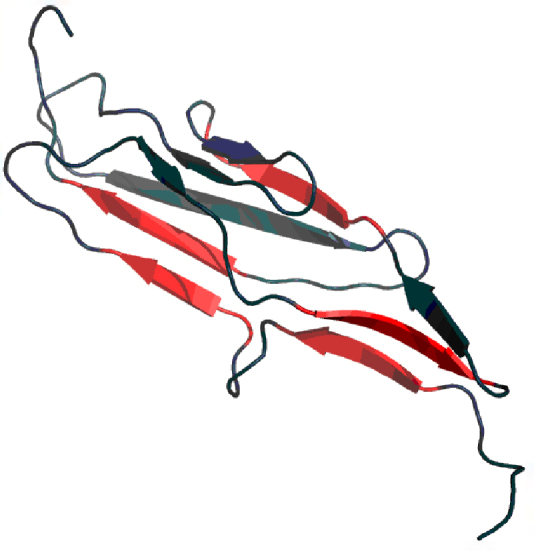
3D presentation of the 2MQC domain. Red fragments represent deviations from the idealized distribution of hydrophobicity.

4. Conclusions and discussion

Each protein molecule is assumed to be synthesized by the cell in order to fulfill a specific biological function. The hydrophobic core − a crucial factor in tertiary structural stabilization − can be found in most proteins. This phenomenon is directly linked to the presence of the water environment in which most proteins are naturally immersed (although membrane proteins are an important exception to this rule). An “ideal” hydrophobic core, represented by a hydrophobicity density distribution profile which matches theoretical values with near-perfect accuracy, would result in excellent solubility, with the entire surface layer of the protein composed of hydrophilic residues. Such conditions can be observed e.g. in antifreeze proteins which must remain soluble but do not directly interact with other molecules [46]. In enzymes, however, local deviations from the idealized profile are expected, and indeed evidenced by our to-date work [42 – page 114, 44 – page 85]. In most cases, elimination of residues engaged in enzymatic activity significantly reduces the value of RD (often to less than 0.5). This suggests that local deformations in the neighbourhood of catalytic residues seem to be intentional and aim-oriented [46]. Regardless of the specific nature of local deformations, their presence appears fundamentally important to the proteins’ biological function. Expanding the existing accuracy criteria with aspects of the fuzzy oil drop model may help acknowledge the impact of the water environment upon the folding process. The structure of the hydrophobic core, emerging as a result of an external force field acting upon the polypeptide chain, is a global phenomenon which cannot be accurately modeled on the level of pairwise atom-atom interactions.

The fuzzy oil drop model can be applied to identify deviations from the idealized structure represented by a 3D Gaussian. We assume that the act of binding a ligand − especially one which docks deep in the protein − requires certain distortions in the core. These distortions render the protein capable of fulfilling its biological role (binding ligands or forming complexes with other proteins) in a specific and targeted fashion.

For the reasons stated above, similarity criteria based on the positions of individual atoms or pairwise interactions between atoms should be expanded with comparative analysis of the protein’s hydrophobic core, requiring correct positioning of all residues which comprise the input chain. The structure of the core, expressed by its observed hydrophobicity density distribution profile, can then be studied to identify local deviations (deficiencies/excesses) from the idealized 3D Gaussian form. This type of analysis has been performed for an arbitrarily selected protein from the CASP11 challenge (T0857). We compared the existing similarity criteria with our proposed FOD method using a set of several distinct models. Following elimination of outliers, the correlation coefficient between CASP and FOD algorithms was 0.828, which indicates that − rather than completely contradicting the official ranking − the FOD method can be treated as an iterative improvement over existing approaches. Note that the presented analysis was restricted to _1 models.

An interesting aspect of the CASP challenge which touches upon the subject of this paper is that participants are generally not informed of any ligands attracted by the target protein − rather, the organizers provide only a rudimentary set of input data, such as the source organism, presence of disulfide bonds etc. One exception to this rule occurred when the structure of the target was so strongly dominated by its ligand that the official description mentioned this fact [10]. It seems that the fuzzy oil drop model may provide clues regarding the potential biological activity of the submitted models, as well as of the target.

The final item on the list of 12 goals of CASP11 states: “Where can future effort be most productively focused?” [47]. In our view, acknowledging the presence of the aqueous environment in structure prediction algorithms helps explain the directed nature of the folding process while also highlighting deviations from the theoretical model which hint upon the potential biological function of target proteins. We believe this phenomenon merits further study.

One of the important open questions in modern protein research can be summarized as follows [48]: “We do not understand why a cellular proteome does not precipitate, despite the high density inside a cell.” We hope that the analysis of the hydrophobic core as defined by the fuzzy oil drop model, i.e. factoring in the hydrophilic shell, may shed some light on this matter. Targeted exposure of hydrophobic residues on the protein surface seems to be a natural way to restrict and control protein complexation.

Recent advances in protein folding research point to the diffusion phenomenon [49], treating solvent viscosity as a potential factor in the folding process; however no definitive theoretical models have yet been published.

Analysis of CASP11 results (July 2016) has provided fresh insight [50, 51], even though model accuracy criteria are still based on existing parameters, such as GDT-TS [52, 53]. The proteins discussed in [54, 55] and characterized − on the basis of crystallographic assessment − as “atypical” provide a useful study group for the fuzzy oil drop model. One example is the monotreme lactation protein (MLP), where the role of the beta-hairpin exposed on the surface may be explained on the grounds of the FOD model. Similarly, the presence of two GLU residues in the interface zone of human vanin 1 is characterized as a local deviation from the theoretical distribution. In PilA1, the major Type IV pilin, the C-terminal fragment exhibits significant discordance versus the model, likely due to its low packing and elasticity. In summary, the Authors would like to point out that symbiotic collaboration between experimental structural biology and computational biology may benefit both disciplines. Indeed, the CASP community has recently reached out to CAPRI to facilitate joint studies into the function/structure relationship, acknowledging that proper identification of protein complexation and ligand binding sites may provide important clues regarding the protein’s biological role [56, 57, 58, 59]. Application of the FOD model to p-p interfaces has revealed some new aspects of complex generation, including the presence of an independent “quasi-domain” comprised of fragments contributed by both chains participating in the complex [60].

It should also be noted that existing model/target similarity criteria are increasingly being called into question − some new proposals in this regard can be found in [61].

One shall underline that the aim of this paper is just presentation of alternative version of similarity measurements. The examples taken from CASP experiment are chosen as the base of correctly and not fully correctly folded proteins to show the applicability of the fuzzy oil drop model.

Fuzzy oil drop model is conditioned by water environment for protein folding. Surprisingly however the molecular dynamics simulation of membrane protein performed in external force field of the ellipsoid capsule appeared to be highly similar to the results obtained as the effect of traditional molecular dynamics simulation in water environment (box with individual water molecules defined explicitly) [62]. This observation proves that the presence of centric concentration of hydrophobic residues seems to universal rule.

The comparable analysis based on fuzzy oil drop model is specially useful for identification of the consequences of mutations introduced in protein molecule [63].

Recently the application of fuzzy oil drop model was used to identify the specificity of amyloid forms [64]. It is shown that the substitution of central concentration of hydrophobicity by linear distribution of hydrophobicity in amyloid fibrils may be the potential mechanism for amyloidogenesis.

Declarations

Author Contribution Statement

Małgorzata Gadzała, Barbara Kalinowska: Contributed reagents, materials, analysis tools or data.

Mateusz Banach: Performed the experiments.

Leszek Konieczny: Conceived and designed the experiments.

Irena Roterman: Conceived and designed the experiments; Analyzed and interpreted the data; Wrote the paper.

Funding statement

This work was supported by Collegium Medicum UJ (K/ZDS/006363) and PLGrid Plus.

Competing interest statement

The authors declare no conflict of interest.

Additional information

No additional information is available for this paper.

References

- 1.CASP Roll July 24, 2016. http://predictioncenter.org
- 2.Venclovas Č., Zemla A., Fidelis K., Moult J. Assessment of progress over the casp experiments. Proteins Str. Func. Gen. 2003;53:585–595. doi: 10.1002/prot.10530. [DOI] [PubMed] [Google Scholar]
- 3.Fisher D., Barret C., Bryson K., Elofsson A., Godzik A., Jones D., Karplus M.J., Kelley L.A., MacCallum R.M., Pawlowski K., Rost B., Rychlewski L., Sterneberg M. CAFASP-1: Critical assessment of Fully automated structure prediction methods. Proteins. 1999;(Suppl. 3):209–217. doi: 10.1002/(sici)1097-0134(1999)37:3+<209::aid-prot27>3.3.co;2-p. [DOI] [PubMed] [Google Scholar]
- 4.Orengo C.A., Bray J.E., Hubbard T., LoConte L., Silitoe I. Analysis and assessment of Ab initio Three-dimensional prediction, secondary structure and contact prediction. Proteins. 1999;(Suppl. 3):149–170. doi: 10.1002/(sici)1097-0134(1999)37:3+<149::aid-prot20>3.3.co;2-8. [DOI] [PubMed] [Google Scholar]
- 5.Lackner P., Koppesteiner W.A., Dominigues F.S., Sippl M.J. Automated large scale evaluation of protein structure. Proteins. 1999;(Suppl. 3):7–14. doi: 10.1002/(sici)1097-0134(1999)37:3+<7::aid-prot3>3.3.co;2-m. [DOI] [PubMed] [Google Scholar]
- 6.Fischer D., Elofsson A., Rychlewski L., Pazos F., Valencia A., Rost B., Ortiz A.R., Dunbrack R.L., Jr. CAFASP2: the second critical assessment of fully automated structure prediction methods. Proteins. 2001;(Suppl. 5):171–183. doi: 10.1002/prot.10036. [DOI] [PubMed] [Google Scholar]
- 7.Venclovas C., Zemla A., Fidelis K., Moult J. Comparison of performance in successive CASP experiments. Proteins. 2001;(Suppl. 5):163–170. doi: 10.1002/prot.10053. [DOI] [PubMed] [Google Scholar]
- 8.Zemla A., Venclovas C., Moult J., Fidelis K. Processing and evaluation of predictions in CASP4. Proteins. 2001;(Suppl. 5):13–21. doi: 10.1002/prot.10052. [DOI] [PubMed] [Google Scholar]
- 9.Moult J., Fidelis K., Zemla A., Hubbard T. Critical assessment of methods of protein structure prediction (CASP): round IV. Proteins. 2001;(Suppl. 5):2–7. [PubMed] [Google Scholar]
- 10.Venclovas C. Comparative modeling In CASP5: Progress is evident: but alignment errors remain a significant hindrance. Proteins. 2003;53:380–388. doi: 10.1002/prot.10591. [DOI] [PubMed] [Google Scholar]
- 11.Venclovas C., Zemla A., Fidelis K., Moult J. Assessment of progress over the CASP experiments. Proteins. 2003;53(Suppl. 6):585–595. doi: 10.1002/prot.10530. [DOI] [PubMed] [Google Scholar]
- 12.Fischer D., Rychlewski L., Dunbrack R.L., Jr., Ortiz A.R., Elofsson A. CAFASP3: the third critical assessment of fully automated structure prediction methods. Proteins. 2003;(Suppl. 6):503–516. doi: 10.1002/prot.10538. [DOI] [PubMed] [Google Scholar]
- 13.Moult J., Fidelis K., Zemla A., Hubbard T. Critical assessment of methods of protein structure prediction (CASP)-round V. Proteins. 2003;(Suppl. 6):334–339. doi: 10.1002/prot.10556. [DOI] [PubMed] [Google Scholar]
- 14.Moult J., Fidelis K., Rost B., Hubbard T., Tramontano A. Critical assessment of methods of protein structure prediction (CASP)-round 6. Proteins. 2005;(Suppl. 7):3–7. doi: 10.1002/prot.20716. [DOI] [PubMed] [Google Scholar]
- 15.Soro S., Tramontano A. The prediction of protein function at CASP6. Proteins. 2005;(Suppl. 7):201–213. doi: 10.1002/prot.20738. [DOI] [PubMed] [Google Scholar]
- 16.Moult J., Fidelis K., Kryshtafovych A., Rost B., Hubbard T., Tramontano A. Critical assessment of methods of protein structure prediction-Round VII. Proteins. 2007;(Suppl. 8):3–9. doi: 10.1002/prot.21767. [DOI] [PMC free article] [PubMed] [Google Scholar]
- 17.Cozzetto D., Kryshtafovych A., Ceriani M., Tramontano A. Assessment of predictions in the model quality assessment category. Proteins. 2007;(Suppl. 8):175–183. doi: 10.1002/prot.21669. [DOI] [PubMed] [Google Scholar]
- 18.Kryshtafovych A., Fidelis K., Moult J. CASP8 results in context of previous experiments. Proteins. 2009;(Suppl. 9):217–228. doi: 10.1002/prot.22562. [DOI] [PMC free article] [PubMed] [Google Scholar]
- 19.Moult J., Fidelis K., Kryshtafovych A., Rost B., Tramontano A. Critical assessment of methods of protein structure prediction - Round VIII. Proteins. 2009;(Suppl. 9):1–4. doi: 10.1002/prot.22589. [DOI] [PubMed] [Google Scholar]
- 20.Kryshtafovych A., Krysko O., Daniluk P., Dmytriv Z., Fidelis K. Protein structure prediction center in CASP8. Proteins. 2009;(Suppl. 9):5–9. doi: 10.1002/prot.22517. [DOI] [PMC free article] [PubMed] [Google Scholar]
- 21.Cozzetto D., Kryshtafovych A., Tramontano A. Evaluation of CASP8 model quality predictions. Proteins. 2009;(Suppl. 9):157–166. doi: 10.1002/prot.22534. [DOI] [PubMed] [Google Scholar]
- 22.MacCallum J.L., Pérez A., Schnieders M.J., Hua L., Jacobson M.P., Dill K.A. Assessment of protein structure refinement in CASP9. Proteins. 2011;(Suppl. 10):74–90. doi: 10.1002/prot.23131. [DOI] [PMC free article] [PubMed] [Google Scholar]
- 23.Moult J., Fidelis K., Kryshtafovych A., Tramontano A. Critical assessment of methods of protein structure prediction (CASP)-round IX. Proteins. 2011;(Suppl. 10):1–5. doi: 10.1002/prot.23200. [DOI] [PMC free article] [PubMed] [Google Scholar]
- 24.Moult J., Fidelis K., Kryshtafovych A., Schwede T., Tramontano A. Critical assessment of methods of protein structure prediction (CASP)-round X. Proteins. 2014;(Suppl. 2):1–6. doi: 10.1002/prot.24452. [DOI] [PMC free article] [PubMed] [Google Scholar]
- 25.Tai C.H., Bai H., Taylor T.J., Lee B. Assessment of template-free modeling in CASP10 and ROLL. Proteins. 2014;(Suppl. 2):57–83. doi: 10.1002/prot.24470. [DOI] [PMC free article] [PubMed] [Google Scholar]
- 26.Kryshtafovych A., Barbato A., Fidelis K., Monastyrskyy B., Schwede T., Tramontano A. Assessment of the assessment: evaluation of the model quality estimates in CASP10. Proteins. 2014;(Suppl. 2):112–126. doi: 10.1002/prot.24347. [DOI] [PMC free article] [PubMed] [Google Scholar]
- 27.Liwo A., Ripoll D.R., Pilardy J., Scheraga H.A. Calculation of protein conformation by global optimization of potential energy function. Proteins. 1999;(Suppl. 3):204–208. doi: 10.1002/(sici)1097-0134(1999)37:3+<204::aid-prot26>3.3.co;2-6. [DOI] [PubMed] [Google Scholar]
- 28.3D structure evaluation - Targets and Domains July 24, 2016. http://www.predictioncenter.org/casprol/results.cgi
- 29.Zemla A. LGA a method for finding 3D similarities in protein structures. Nucleic Acids Res. 2003;31(13):3370–3374. doi: 10.1093/nar/gkg571. [DOI] [PMC free article] [PubMed] [Google Scholar]
- 30.Global Distance Test July 24, 2016. https://en.wikipedia.org/wiki/Global_distance_test
- 31.Cong Q., Kinch L.N., Pei J., Shi S., Grishin V.N., Li W., Grishin N.V. An automatic method for CASP9 free modeling structure prediction assessment. Bioinformatics. 2011;27(24):3371–3378. doi: 10.1093/bioinformatics/btr572. [DOI] [PMC free article] [PubMed] [Google Scholar]
- 32.Holm L., Sander C. Protein structure comparison by alignment of distance matrices. J. Mol. Biol. 1993;233(1):123–138. doi: 10.1006/jmbi.1993.1489. [DOI] [PubMed] [Google Scholar]
- 33.Mariani V., Kiefer F., Schmidt T., Haas J., Schwede T. Assessment of template based protein structure predictions in CASP9. Proteins. 2011;(Suppl. S10):37–58. doi: 10.1002/prot.23177. [DOI] [PubMed] [Google Scholar]
- 34.Olechnovič K., Kulberkytė E., Venclovas C. CAD-score a new contact area difference-based function for evaluation of protein structural models. Proteins. 2013;81(1):149–162. doi: 10.1002/prot.24172. [DOI] [PubMed] [Google Scholar]
- 35.Keedy D.A., Williams C.J., Headd J.J., Arendall 3rd W.B., Chen V.B., Kapral G.J., Gillespie R.A., Block J.N., Zemla A., Richardson D.C., Richardson J.S. The other 90% of the protein: Assessment beyond the Cαs for CASP8 template-based and high-accuracy models. Proteins. 2009;(Suppl. 9):29–49. doi: 10.1002/prot.22551. [DOI] [PMC free article] [PubMed] [Google Scholar]
- 36.Laskowski R.A. Enhancing the functional annotation of PDB structures in PDBsum using key figures extracted from the literature. Bioinformatics. 2007;23:1824–1827. doi: 10.1093/bioinformatics/btm085. [DOI] [PubMed] [Google Scholar]
- 37.Kauzmann W. Some factors in the interpretation of protein denaturation. Adv. Protein Chem. 1959;14:1–63. doi: 10.1016/s0065-3233(08)60608-7. [DOI] [PubMed] [Google Scholar]
- 38.Chiche L., Gregoret L.M., Cohen F.E., Kollman P.A. Protein model structure evaluation using the solvation free energy of folding. Proc. Natl. Acad. Sci. USA. 1990;87:3240–3243. doi: 10.1073/pnas.87.8.3240. [DOI] [PMC free article] [PubMed] [Google Scholar]
- 39.Kalinowska B., Banach M., Konieczny L., Roterman I. Application of Divergence Entropy to Characterize the Structure of the Hydrophobic Core in DNA Interacting Proteins. Entropy. 2015;17(3):1477–1507. [Google Scholar]
- 40.Levitt M. A simplified representation of protein conformations for rapid simulation of protein folding. J. Mol. Biol. 1976;104:59–107. doi: 10.1016/0022-2836(76)90004-8. [DOI] [PubMed] [Google Scholar]
- 41.Kulback S., Leibler R.A. On information and sufficiency. Ann. Math. Stat. 1951;22:79–86. [Google Scholar]
- 42.Kalinowska B., Banach M., Konieczny L., Marchewka D., Roterman I. Intrinsically disordered proteins–relation to general model expressing the active role of the water environment. Adv. Protein Chem. Struct. Biol. 2014;94:315–346. doi: 10.1016/B978-0-12-800168-4.00008-1. [DOI] [PubMed] [Google Scholar]
- 43.Banach M., Konieczny L., Roterman I. Use of the fuzzy oil drop model to identify the complexation area in protein homodimers. In: Irena Roterman-Konieczna, editor. Protein folding in silico - Protein folding versus protein structure prediction. Woodhead Publishing (Currently: Elsevier); Oxford, Cambridge, Philadelphia, New Delhi: 2012. pp. 95–122. [Google Scholar]
- 44.Banach M., Konieczny L., Roterman I. Ligand-binding site recognition. In: Irena Roterman-Konieczna, editor. Protein folding in silico - Protein folding versus protein structure prediction. Woodhead Publishing (Currently: Elsevier); Oxford, Cambridge, Philadelphia, New Delhi: 2012. pp. 79–94. [Google Scholar]
- 45.Roterman-Konieczna Irena, editor. Springer; Dordrecht, Heidelberg, New York, London: 2013. Identification of ligand binding and protein-protein interaction area. [Google Scholar]
- 46.Banach M., Konieczny L., Roterman I. The fuzzy oil drop model: based on hydrophobicity density distribution generalizes the influence of water environment on protein structure and function. J. Theor. Biol. 2014;21(359):6–17. doi: 10.1016/j.jtbi.2014.05.007. [DOI] [PubMed] [Google Scholar]
- 47.CASP Roll July 17, 2016. http://predictioncenter.org/casp11/index.cgi
- 48.Dill K.A., MacCallum J.L. The protein-folding problem 50 years on. Science. 2012;338:1042–1046. doi: 10.1126/science.1219021. [DOI] [PubMed] [Google Scholar]
- 49.Chung H.S., Piana-Agostinetti S., Shaw D.E., Eaton W.A. Structural origin of slow diffusion in protein folding. Science. 2015;349:1504–1510. doi: 10.1126/science.aab1369. [DOI] [PMC free article] [PubMed] [Google Scholar]
- 50.Modi V., Dunbrack R.L., Jr. Assessment of refinement of template-based models in CASP11. Proteins. 2016;(Suppl. 1):260–281. doi: 10.1002/prot.25048. [DOI] [PMC free article] [PubMed] [Google Scholar]
- 51.Moult J., Fidelis K., Kryshtafovych A., Schwede T., Tramontano A. Critical assessment of methods of protein structure prediction: Progress and new directions in round XI. Proteins. 2016;(Suppl. 1):4–14. doi: 10.1002/prot.25064. [DOI] [PMC free article] [PubMed] [Google Scholar]
- 52.Cao R., Cheng J. Protein single-model quality assessment by feature-based probability density functions. Sci. Rep. 2016;6:23990. doi: 10.1038/srep23990. [DOI] [PMC free article] [PubMed] [Google Scholar]
- 53.Belsom A., Schneider M., Brock O., Rappsilber J. Blind Evaluation of Hybrid Protein Structure Analysis Methods based on Cross-Linking. Trends Biochem. Sci. 2016;41(7):564–567. doi: 10.1016/j.tibs.2016.05.005. [DOI] [PMC free article] [PubMed] [Google Scholar]
- 54.Kryshtafovych A., Moult J., Bartual S.G., Bazan J.F., Berman H., Casteel D.E., Christodoulou E., Everett J.K., Hausmann J., Heidebrecht T., Hills T., Hui R., Hunt J.F., Seetharaman J., Joachimiak A., Kennedy M.A., Kim C., Lingel A., Michalska K., Montelione G.T., Otero J.M., Perrakis A., Pizarro J.C., van Raaij M.J., Ramelot T.A., Rousseau F., Tong L., Wernimont A.K., Young J., Schwede T. Target highlights in CASP9: Experimental target structures for the critical assessment of techniques for protein structure prediction. Proteins. 2016;(Suppl. 1):34–50. doi: 10.1002/prot.23196. [DOI] [PMC free article] [PubMed] [Google Scholar]
- 55.Kryshtafovych A., Moult J., Baslé A., Burgin A., Craig T.K., Edwards R.A., Fass D., Hartmann M.D., Korycinski M., Lewis R.J., Lorimer D., Lupas A.N., Newman J., Peat T.S., Piepenbrink K.H., Prahlad J., van Raaij M.J., Rohwer F., Segall A.M., Seguritan V., Sundberg E.J., Singh A.K., Wilson M.A., Schwede T. Some of the most interesting CASP11 targets through the eyes of their authors. Proteins. 2016;(Suppl. 1):34–50. doi: 10.1002/prot.24942. [DOI] [PMC free article] [PubMed] [Google Scholar]
- 56.Vangone A., Rodrigues J.P., Xue L.C., van Zundert G.C., Geng C., Kurkcuoglu Z., Nellen M., Narasimhan S., Karaca E., van Dijk M., Melquiond A.S., Visscher K.M., Trellet M., Kastritis P.L., Bonvin A.M. Sense and Simplicity in HADDOCK Scoring: Lessons from CASP-CAPRI Round1. Proteins. 2016 doi: 10.1002/prot.25339. [DOI] [PMC free article] [PubMed] [Google Scholar]
- 57.Vangone A., Rodrigues J.P., Xue L.C., van Zundert G.C., Geng C., Kurkcuoglu Z., Nellen M., Narasimhan S., Karaca E., van Dijk M., Melquiond A.S., Visscher K.M., Trellet M., Kastritis P.L., Bonvin A.M. Prediction of homoprotein and heteroprotein complexes by protein docking and template-based modeling: A CASP-CAPRI experiment. Proteins. 2016 doi: 10.1002/prot.25007. [DOI] [PMC free article] [PubMed] [Google Scholar]
- 58.Roche D.B., McGuffin L.J. In silico Identification and Characterization of Protein-Ligand Binding Sites. Methods Mol. Biol. 2016;1414:1–21. doi: 10.1007/978-1-4939-3569-7_1. [DOI] [PubMed] [Google Scholar]
- 59.Roche D.B., Brackenridge D.A., McGuffin L.J. Proteins and Their Interacting Partners: An Introduction to Protein-Ligand Binding Site Prediction Methods. Int. J. Mol. Sci. 2015;16(12):29829–29842. doi: 10.3390/ijms161226202. [DOI] [PMC free article] [PubMed] [Google Scholar]
- 60.Dygut J., Kalinowska B., Banach M., Piwowar M., Konieczny L., Roterman I. Structural Interface Forms and Their Involvement in Stabilization of Multidomain Proteins or Protein Complexes. Int. J. Mol. Sci. 2016;17(10) doi: 10.3390/ijms17101741. [DOI] [PMC free article] [PubMed] [Google Scholar]
- 61.Li W., Schaeffer R.D., Otwinowski Z., Grishin N.V. Estimation of Uncertainties in the Global Distance Test (GDT_TS) for CASP Models. PLoS One. 2016;11(5) doi: 10.1371/journal.pone.0154786. eCollection 2016. [DOI] [PMC free article] [PubMed] [Google Scholar]
- 62.Zobnina V., Roterman I. Application of the fuzzy-oil-drop model to membrane protein simulation. Proteins. 2009;77(2):378–394. doi: 10.1002/prot.22443. [DOI] [PubMed] [Google Scholar]
- 63.Banach M., Prymula K., Jurkowski W., Konieczny L., Roterman I. Fuzzy oil drop model to interpret the structure of antifreeze proteins and their mutants. J. Mol. Model. 2012;18(1):229–237. doi: 10.1007/s00894-011-1033-4. [DOI] [PMC free article] [PubMed] [Google Scholar]
- 64.Roterman I., Banach M., Kalinowska B., Konieczny L. Influence of the Aqueous Environment on Protein Structure - A Plausible Hypothesis Concerning the Mechanism of Amyloidogenesis. Entropy. 2016;18(10):351. [Google Scholar]