Mapping Lifetime Brain Volumetry with Covariate-Adjusted Restricted Cubic Spline Regression from Cross-sectional Multi-site MRI

Abstract

Understanding brain volumetry is essential to understand neurodevelopment and disease. Historically, age-related changes have been studied in detail for specific age ranges (e.g., early childhood, teen, young adults, elderly, etc.) or more sparsely sampled for wider considerations of lifetime aging. Recent advancements in data sharing and robust processing have made available considerable quantities of brain images from normal, healthy volunteers. However, existing analysis approaches have had difficulty addressing (1) complex volumetric developments on the large cohort across the life time (e.g., beyond cubic age trends), (2) accounting for confound effects, and (3) maintaining an analysis framework consistent with the general linear model (GLM) approach pervasive in neuroscience. To address these challenges, we propose to use covariate-adjusted restricted cubic spline (C-RCS) regression within a multi-site cross-sectional framework. This model allows for flexible consideration of non-linear age-associated patterns while accounting for traditional covariates and interaction effects. As a demonstration of this approach on lifetime brain aging, we derive normative volumetric trajectories and 95% confidence intervals from 5111 healthy patients from 64 sites while accounting for confounding sex, intracranial volume and field strength effects. The volumetric results are shown to be consistent with traditional studies that have explored more limited age ranges using single-site analyses. This work represents the first integration of C-RCS with neuroimaging and the derivation of structural covariance networks (SCNs) from a large study of multi-site, cross-sectional data.

1 Introduction

Brain volumetry across the lifespan is essential in neurological research and clinical investigation. Magnetic resonance imaging (MRI) allows for quantification of such changes, and consequent investigation of specific age ranges or more sparsely sampled lifetime data [1]. Contemporaneous advancements in data sharing have made considerable quantities of brain images available from normal, healthy populations. However, the regression models prevalent in volumetric mapping (e.g., liner, polynomial, non-parametric model, etc.) have had difficulty in modeling complex, cross-sectional large cohorts while accounting for confound effects.

This paper proposes a novel multi-site cross-sectional framework using Covariate-adjusted Restricted Cubic Spline (C-RCS) regression to map brain volumetry on a large cohort (5111 MR 3D images) across the lifespan (4~98 years). The C-RCS extends the Restricted Cubic Spline [2, 3] by regressing out the confound effects in a general linear model (GLM) fashion. Multi-atlas segmentation is used to obtain whole brain volume (WBV) and 132 regional volumes. The regional volumes are further grouped to 15 networks of interest (NOIs). Then, structural covariance networks (SCNs), i.e. regions or networks that mature or decline together during developmental periods, are established based on NOIs using hierarchical clustering analysis (HCA). To validate the large-scale framework, confidence intervals (CI) are provided for both C-RCS regression and clustering from 10,000 bootstrap samples.

2 Methods

2.1 Extracting Volumetric Information

The complete cohort aggregates 9 datasets with a total 5111 MR T1w 3D images from normal healthy subjects (Table 1). 45 atlases are non-rigidly registered [4] to a target image and non-local spatial staple (NLSS) label fusion [5] is used to fuse the labels from each atlas to the target image using the BrainCOLOR protocol [6] (Fig. 1). WBV and regional volume are then calculated by multiplying the volume of a single voxel by the number of labeled voxels in original image space. In total, 15 NOIs are defined by structural and functional covariance networks including visual, frontal, language, memory, motor, fusiform, basal ganglia (BG) and cerebellum (CB).

Table 1.

Data summary of 5111 multi-site images.

Study Name	Website	Images	Sites
Baltimore Longitudinal Study of Aging (BLSA)	http://www.blsa.nih.gov	605	4
Cutting Pediatrics	http://vkc.mc.vanderbilt.edu/ebrl	586	2
Autism Brain Imaging Data Exchange (ABIDE)	http://fcon_1000.projects.nitrc.org/indi/abide	563	17
Information eXtraction from Images (IXI)	http://www.nitrc.org/projects/ixi_dataset	523	3
Attention Deficit Hyperactivity Disorder (ADHD200)	http://fcon_1000.projects.nitrc.org/indi/adhd200	949	8
National Database for Autism Research (NDAR)	http://ndar.nih.gov	328	6
Open Access Series on Imaging Study (OASIS)	http://www.oasis-brains.org	312	1
1000 Functional Connectome (fcon_1000)	http://fcon_1000.projects.nitrc.org	1102	22
Nathan Kline Institute Rockland (NKI_rockland)	http://fcon_1000.projects.nitrc.org/indi/enhanced	143	1

Fig. 1.

The large-scale cross-sectional framework on 5111 multi-site MR 3D images.

2.2 Covariate-Adjusted Restricted Cubic Spline (C-RCS)

We define x as the ages of all subjects and S (x)as the corresponding brain volumes. In canonical nth degree spline regression, splines are used to model non-linear relationships between variables S (x) and x by deciding the connections between K knots (t₁ < t₂ < ⋯ < t_K). In this work, such knots were determined based on previously identified developmental shifts [1], specifically corresponding with transitions between childhood (7–12), late adolescence (12–19), young adulthood (19–30), middle adulthood (30–55), older adulthood (55–75), and late life (75–90). Using the expression from Durrleman [2], the canonical nth degree spline function is defined as

$$S(x)={\sum }_{j=0}^n{\dot{\beta }}_{oj}{x}^j+{\sum }_{i=1}^K{\dot{\beta }}_{\mathit{\text{in}}}{(x-t_i)}_{+}^n$$ (1)

where (x −t_i)₊ = x − t_i, if x > t_i; (x − t_i)₊ = 0, if x ≤ t_i.

To regress out confound effects, new covariates $X_1^{\text{'}},X_2^{\text{'}},\dots ,X_c^{\text{'}}$ (with coefficients ${\beta }_1^{\text{'}},{\beta }_2^{\text{'}},\dots ,{\beta }_c^{\text{'}}$ are introduced to the nth degree spline regression

$$S(x)={\sum }_{j=0}^n{\dot{\beta }}_{oj}{x}^j+{\sum }_{i=1}^K{\dot{\beta }}_{\mathit{\text{in}}}{(x-t_i)}_{+}^n+{\sum }_{u=0}^C{\beta }_u^{\text{'}}{X}_u^{\text{'}}$$ (2)

where C is the number of confound effects.

In the RCS regression, a linear constrain is introduced [2] to address the poor behavior of the cubic spline model in the tails (x < t₁ and x > t_K)[7]. Using the same principle, C-RCS regression extends the RCS regression (n = 3) and restricts the relationship between S (x) and x to be a linear function in the tails. First, for x < t₁,

$$S(x)={\dot{\beta }}_{00}+{\dot{\beta }}_{01}x+{\dot{\beta }}_{02}{x}^2+{\dot{\beta }}_{03}{x}^3+{\dot{\beta }}_{13}+{\sum }_{u=0}^C{\beta }_u^{\text{'}}{X}_u^{\text{'}}$$ (3)

where β̇₀₂ = β̇₀₃ = 0 ensures the linearity before the first knot. Second, for x > t_K,

$$S(x)={\dot{\beta }}_{00}+{\dot{\beta }}_{01}x+{\dot{\beta }}_{13}{(x-t_1)}_{+}^3+\cdots +{\dot{\beta }}_{K3}{(x-t_K)}_{+}^3+{\sum }_{u=0}^C{\beta }_u^{\text{'}}{X}_u^{\text{'}}$$ (4)

To guarantee the linearity of C-RCS after the last knot, we expand the previous expression and force the coefficients of x² and x³ to be zero. After expansion,

$$S(x)=({\dot{\beta }}_{00}+{\dot{\beta }}_{13}{t}_1^3+\cdots +{\dot{\beta }}_{K3}{t}_K^3+{\sum }_{u=0}^C{\beta }_u^{\text{'}}{X}_u^{\text{'}})+({\dot{\beta }}_{01}+3{\dot{\beta }}_{13}{t}_1^2+\cdots +3{\dot{\beta }}_{K3}{t}_K^2)x+(3{\dot{\beta }}_{13}{t}_1+3{\dot{\beta }}_{23}{t}_2+\cdots +3{\dot{\beta }}_{K3}{t}_K)x^2+(3{\dot{\beta }}_{13}+3{\dot{\beta }}_{23}+\cdots +3{\dot{\beta }}_{K3})x^3$$ (5)

As a result, linearity of S (x)at x > t_K implies that ${\sum }_{i=1}^K{\dot{\beta }}_{i3}{t}_i=0$ and ${\sum }_{i=1}^K{\dot{\beta }}_{i3}=0$. Following such restrictions, the β̇_(K−1)3 and β̇_K³ are derived as

$${\dot{\beta }}_{(K-1)3}=-\frac{{\sum }_{i=1}^{K-2}{\dot{\beta }}_{i3}(t_K-t_i)}{t_K-t_{K-1}}\text{ and }{\dot{\beta }}_{K3}=\frac{{\sum }_{i=1}^{K-2}{\dot{\beta }}_{i3}(t_{K-1}-t_i)}{t_K-t_{K-1}}$$ (6)

and the complete C-RCS regression model is defined as

$$S(x)={\dot{\beta }}_{00}+{\dot{\beta }}_{01}x+{\sum }_{i=1}^{K-2}{\dot{\beta }}_{i3}[{(x-t_i)}_{+}^3-\frac{t_K-t_i}{t_K-t_{K-1}}{(x-t_{K-1})}_{+}^3+\frac{t_{K-1}-t_i}{t_K-t_{K-1}}{(x-t_K)}_{+}^3]+{\sum }_{u=0}^C{\beta }_u^{\text{'}}{X}_u^{\text{'}}$$ (7)

2.3 Regressing Out Confound Effects by C-RCS Regression in GLM Fashion

To adapt C-RCS regression in the GLM fashion, we redefine the coefficients β₀, β₁, β₂, …, β_K−1, as Harrell [3] where β₀ = β̇₀₀, β₁ = β̇₀₁, β₂ = β̇₁₃, β₃ = β̇₂₃, β₄ = β̇₃₃, ⋯, β_(K−1)3. Then, the C-RCS regression with confound effects becomes

$$S(x)={\beta }_0+{\sum }_{j=1}^{K-1}{\beta }_j{X}_j+{\sum }_{u=0}^C{\beta }_u^{\text{'}}{X}_u^{\text{'}}$$ (8)

where C is the number for all confound effects $(X_u^{\text{'}})$. X₁ = x and for j = 2, …, K − 1

$$X_j={(x-t_{j-1})}_{+}^3-\frac{t_K-t_{j-1}}{t_K-t_{K-1}}{(x-t_{K-1})}_{+}^3+\frac{t_{K-1}-t_{j-1}}{t_K-t_{K-1}}{(x-t_K)}_{+}^3$$ (9)

Then, the beta coefficients are solvable under GLM framework. Once β̂₀, β̂₁, β̂₂, ⋯, β̂_K−1 are obtained, two linear assured terms β̂_K and β̂_K+1 are estimated:

$${\hat{\beta }}_K=\frac{{\sum }_{i=2}^{K-1}{\hat{\beta }}_i(t_{i-1}-t_K)}{t_K-t_{K-1}}\text{ and }{\hat{\beta }}_{K+1}=\frac{{\sum }_{i=2}^{K-1}{\hat{\beta }}_i(t_{i-1}-t_{K-1})}{t_{K-1}-t_K}$$ (10)

The final estimated volumetric trajectories Ŝ (x) can be fitted as

$$\hat{S}(x)={\hat{\beta }}_0+{\sum }_{j=1}^{K+1}{\hat{\beta }}_j{(x-t_j)}_{+}^3+{\sum }_{u=0}^C{\hat{\beta }}_u^{\text{'}}{X}_u^{\text{'}}$$ (11)

In this work, gender, field strength and total intracranial volume (TICV) are employed as covariates $X_u^{\text{'}}$. TICV values are calculated using SIENAX [8]. Field strength and TICV are used to regress out site effects rather than using site categories directly since the sites are highly correlated with the explanatory variable age.

2.4 SCNs and CI using Bootstrap Method

Using aforementioned C-RCS regression, the lifespan volumetric trajectories of WBV and 15 NOIs are obtained from 5111 images. Simultaneously, the piecewise volumetric trajectories within a particular age bin (between adjacent knots) of all 15 NOIs (Ŝ_i (x), i = 1,2, …, 15) are separated to establish SCNs dendrograms using HCA [9]. The distance metric D used in HCA is defined as D = 1 − corr(Ŝ_i (x), Ŝ_j (x)), i,j ∈ [1,2, …,15] and i ≠ j, where corr(·) is the Pearson's correlation between any two C-RCS fitted piecewise trajectories Ŝ_i (x)and Ŝ_j (x)in the same age bin.

The stability of proposed approaches is demonstrated by the CIs of C-RCS regression and SCNs using bootstrap method [10]. First, the 95% CIs of volumetric trajectories on WBV (Fig. 2) and 15 NOIs (Fig. 3) are derived by deploying C-RCS regression on 10,000 bootstrap samples. Then, the distances D between all pairs of clustered NOIs are derived using 15 (NOIs) × 10,000 (bootstrap) C-RCS fitted trajectories. Then, the 95% CIs are obtained for each pair of clustered NOIs and shown on six SCNs dendrograms (Fig. 4). The average network distance (AND), the average distance between 15 NOIs for a dendrogram, can be calculated 10,000 times using bootstrap. The AND reflects the modularity of connections between all NOIs. We are able to see if the AND are significantly different during brain development periods by deploying the two-sample t-test on AND values (10,000/age bin) between age bins.

Fig. 2.

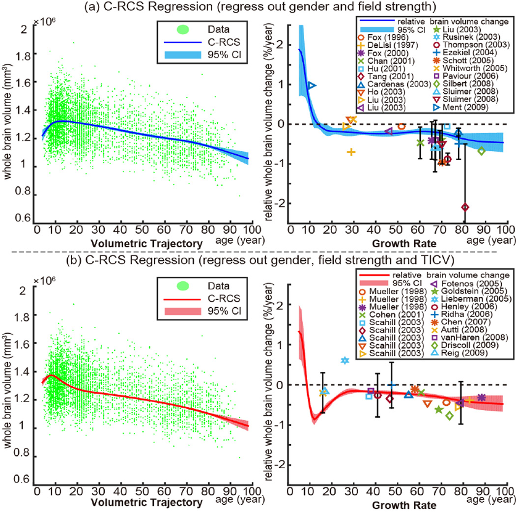
Volumetry and growth rate. The left plot in (a) shows the volumetric trajectory of whole brain volume (WBV) using C-RCS regression on 5111 MR images. The right figure in (a) indicates the growth rate curve, which shows volumetric change per year of the volumetric trajectory. In (b), C-RCS regression is deployed on the same dataset by additionally regressing out TICV. Our growth rate curves are compared with 40 previous longitudinal studies [1] on smaller cohorts (21 studies in (a) without regressing out TICV and 19 studies in (b) regressing out TICV). The standard deviations of previous studies are provided as black bars (if available). The 95% CIs in all plots are calculated from 10,000 bootstrap samples.

Fig. 3.

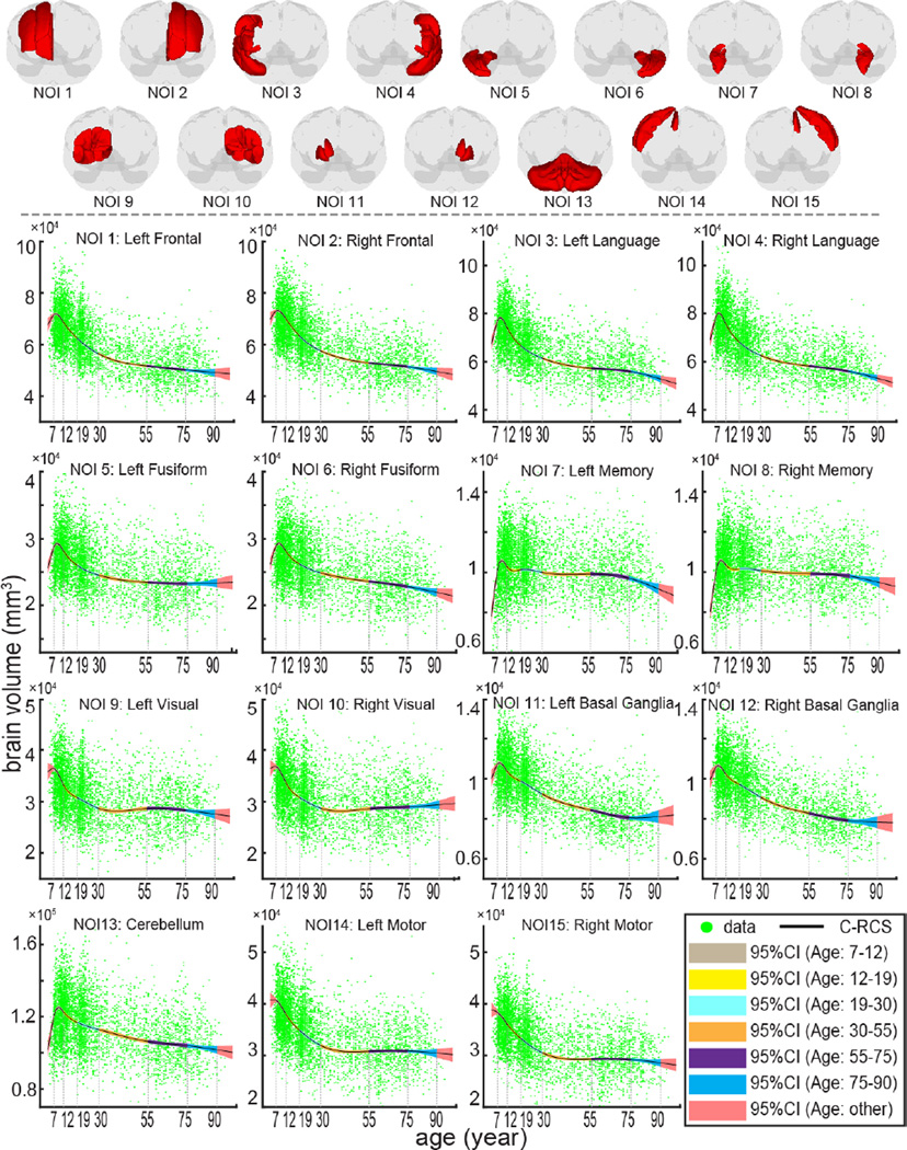
Lifespan trajectories of 15 NOIs are provided with 95% CI from 10,000 bootstrap samples. The upper 3D figures indicate the definition of NOIs (in red). The lower figures show the trajectories with CI using C-RCS regression method by regressing out gender, field strength and TICV (same model as Fig. 2b). For each NOI, the piecewise CIs of six age bins are shown in different colors. The piecewise volumetric trajectories and CIs are separated by 7 knots in the lifespan C-RCS regression rather than conducting independent fittings. The volumetric trajectories on both sides of each NOI are derived separately except for CB.

Fig. 4.

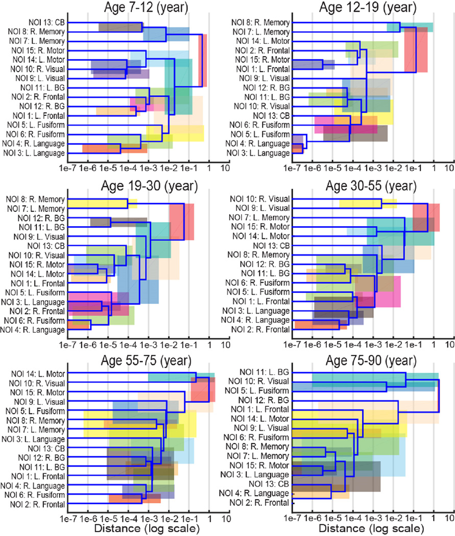
The six structural covariance networks (SCNs) dendrograms using hierarchical clustering analysis (HCA) indicate which NOIs develop together during different developmental periods (age bins). The distance on the x-axis is in log scale, which equals to one minus Pearson’s correlation between two curves. The correlation between NOIs becomes stronger from right to left on the x-axis. The horizontal range of each colored rectangles indicates the 95% CI of distance from 10,000 bootstrap samples. Note that the colors are chosen for visualization purposes without quantitative meanings.

3 Results

Fig. 2a shows the lifespan volumetric trajectories using C-RCS regression as well as the growth rate (volume change in percentage per year) of WBV when regressing out gender and field strength effects. Fig. 2b indicates the C-RCS regression on the same dataset by adding TICV as an additional covariate. The cross sectional growth rate curve using C-RCS regression is compared with 40 previous longitudinal studies (19 are TICV corrected) [1], which are typically limited on smaller age ranges.

Using the same C-RCS model in Fig. 2b, Fig. 3 indicates the both lifespan and piecewise volumetric trajectories of 15 NOIs. In Fig. 4, the piecewise volumetric trajectories of the 15 NOIs within each age bin are clustered using HCA and shown in one SCNs dendrogram.

Then, six SCNs dendrograms are obtained by repeating HCA on different age bins, which demonstrate the evolution of SCNs during different developmental periods. The ANDs between any two age bins in Fig. 4 are statistically significant (p<0.001).

4 Conclusion and Discussion

This paper proposes a large-scale cross-sectional framework to investigate life-time brain volumetry using C-RCS regression. C-RCS regression captures complex brain volumetric trajectories across the lifespan while regressing out confound effects in a GLM fashion. Hence, it can be used by researchers within a familiar context. The estimated volume trends are consistent with 40 previous smaller longitudinal studies. The stable estimation of volumetric trends for NOI (exhibited by narrow confidence bands) provides a basis for assessing patterns in brain changes through SCNs. Moreover, we demonstrate how to compute confidence intervals for SCNs and correlations between NOIs. The significant difference of AND indicates that the C-RCS regression detects the changes of average SCNs connections during the brain development.

Emerging “big data” studies need a regression that is able to capture the complicated lifespan brain development without unnecessarily sacrificing power. The proposed C-RCS regression is a such framework that addresses age-range analyses and varied neuroanatomical regions of interest. To the best of our knowledge, this is the first work that uses C-RCS to quantify temporal changes in SCNs using brain volumetry with a cross-sectional, multi-site paradigm. The challenge of using C-RCS method is that the knots should be defined properly. The software is freely available online¹.

References

- 1.Hedman AM, van Haren NE, Schnack HG, Kahn RS, Hulshoff Pol HE. Human brain changes across the life span: a review of 56 longitudinal magnetic resonance imaging studies. Human brain mapping. 2012;33:1987–2002. doi: 10.1002/hbm.21334. [DOI] [PMC free article] [PubMed] [Google Scholar]
- 2.Durrleman S, Simon R. Flexible regression models with cubic splines. Statistics in medicine. 1989;8:551–561. doi: 10.1002/sim.4780080504. [DOI] [PubMed] [Google Scholar]
- 3.Harrell F. Regression modeling strategies: with applications to linear models, logistic and ordinal regression, and survival analysis. Springer; 2015. [Google Scholar]
- 4.Avants BB, Epstein CL, Grossman M, Gee JC. Symmetric diffeomorphic image registration with cross-correlation: evaluating automated labeling of elderly and neurodegenerative brain. Medical image analysis. 2008;12:26–41. doi: 10.1016/j.media.2007.06.004. [DOI] [PMC free article] [PubMed] [Google Scholar]
- 5.Asman AJ, Dagley AS, Landman BA. Statistical label fusion with hierarchical performance models. Proceedings - Society of Photo-Optical Instrumentation Engineers. 2014;9034:90341E. doi: 10.1117/12.2043182. [DOI] [PMC free article] [PubMed] [Google Scholar]
- 6.Klein A, Dal Canton T, Ghosh SS, Landman B, Lee J, Worth A. Open labels: online feedback for a public resource of manually labeled brain images. 16th Annual Meeting for the Organization of Human Brain Mapping. 2010 [Google Scholar]
- 7.Stone CJ, Koo C-Y. Additive splines in statistics. 1986:48. [Google Scholar]
- 8.Smith SM, Zhang Y, Jenkinson M, Chen J, Matthews PM, Federico A, De Stefano N. Accurate, robust, and automated longitudinal and cross-sectional brain change analysis. Neuroimage. 2002;17:479–489. doi: 10.1006/nimg.2002.1040. [DOI] [PubMed] [Google Scholar]
- 9.Anderberg MR. Cluster analysis for applications: probability and mathematical statistics: a series of monographs and textbooks. Academic press; 2014. [Google Scholar]
- 10.Efron B, Tibshirani RJ. An introduction to the bootstrap. CRC press. 1994 [Google Scholar]