

Abstract
A well-known problem in ultra-high-field MRI is generation of high-resolution three-dimensional images for detailed characterization of white and gray matter anatomical structures. T1-weighted imaging traditionally used for this purpose suffers from the loss of contrast between white and gray matter with an increase of magnetic field strength. Macromolecular proton fraction (MPF) mapping is a new method potentially capable to mitigate this problem due to strong myelin-based contrast and independence of this parameter of field strength. MPF is a key parameter determining the magnetization transfer effect in tissues and defined within the two-pool model as a relative amount of macromolecular protons involved into magnetization exchange with water protons. The objectives of this study were to characterize the two-pool model parameters in brain tissues in ultra-high magnetic fields and introduce fast high-field 3D MPF mapping as both anatomical and quantitative neuroimaging modality for small animal applications. In vivo imaging data were obtained from four adult male rats using an 11.7T animal MRI scanner. Comprehensive comparison of brain tissue contrast was performed for standard R1 and T2 maps and reconstructed from Z-spectroscopic images two-pool model parameter maps including MPF, cross-relaxation rate constant, and T2 of pools. Additionally, high-resolution whole-brain 3D MPF maps were obtained with isotropic 170 μm voxel size using the single-point synthetic-reference method. MPF maps showed 3–6-fold increase in contrast between white and gray matter compared to other parameters. MPF measurements by the single-point synthetic reference method were in excellent agreement with the Z-spectroscopic method. MPF values in rat brain structures at 11.7T were similar to those at lower field strengths, thus confirming field independence of MPF. 3D MPF mapping provides a useful tool for neuroimaging in ultra-high magnetic fields enabling both quantitative tissue characterization based on the myelin content and high-resolution neuroanatomical visualization with high contrast between white and gray matter.
Keywords: High-field MRI, Macromolecular proton fraction (MPF), Neuroimaging, Rat brain
Graphical abstract
1. Introduction
An increase of magnetic field strength in MRI offers improvements of contrast in certain applications including functional, perfusion, and susceptibility-weighted imaging and a greater signal-to-noise ratio (SNR), which potentially can be converted into higher spatial resolution (Balchandani and Naidich, 2015; Lövblad et al., 2012; Ugurbil, 2014). However, imaging in ultra-high magnetic fields imposes a number of challenges, such as increased non-uniformity of B0 and B1 fields, larger specific absorption rate (SAR), more pronounced magnetic susceptibility artifacts, and changes in relaxation properties of tissues. A well-known problem in ultrahigh-field MRI is a decrease of T1-weighted tissue contrast with an increase of field strength (Balchandani and Naidich, 2015; de Graaf et al., 2006; van de Ven et al., 2007; Pohmann et al., 2011; Kara et al., 2013). For this reason, T2-weighted imaging remains the only suitable modality for routine neuroanatomical applications in magnetic fields beyond 9–10 T. However, high-field T2-weighted imaging has some limitations in the morphological context. T2-weighted images are typically acquired using a sequence with multiple spin-echo readout (RARE or FSE). T2 shortening in high fields precludes using large acceleration factors in this sequence due to degradation of image quality caused by point spread function broadening. In combination with a long repetition time (TR) required for T2-weighting, 3D T2-weighted imaging with sufficiently high resolution in all directions becomes prohibitively time-consuming for most small animal neuroimaging applications in vivo. Additionally, T2-weighted imaging in high fields becomes very sensitive to the magnetic susceptibility effect caused by the presence of super-paramagnetic substances. This effect may result in obscuring anatomical details in cell labeling applications or in the presence of hemorrhage after surgical procedures. As such, small animal MRI in ultra-high magnetic fields is essentially lacking a technique that could afford high-resolution 3D visualization of brain morphology in vivo with minimal sensitivity to the susceptibility and paramagnetic effects and positive contrast between white matter (WM) and gray matter (GM).
One contrast mechanism that is potentially capable to mitigate contrast generation problems in ultra-high magnetic fields is the magnetization transfer (MT) effect. MT is frequently characterized by empirical semi-quantitative indexes describing changes in the signal intensity caused by radiofrequency saturation that is partially selective to the resonance of macromolecular protons. Examples of such indexes include MT ratio (MTR) (Dousset et al., 1992), MT saturation (MTsat) (Helms et al., 2008), and MTR difference observed in the recently proposed inhomogeneous MT experimental method (ihMTR) (Varma et al., 2015a). Some of these quantities, such as MTsat (Boretius et al., 2010) and ihMTR (Prevost et al., 2016) showed a promise in ultra-high field anatomical neuroimaging due to their capability to generate strong contrast between WM and GM on corresponding parametric maps. However, the above indexes are problematic to use for the objective quantitative characterization of pathological changes in tissues due to their complex dependence on the parameters of an imaging sequence and underlying biophysical model describing the MT effect. Alternatively, the MT effect can be characterized by a set of relaxation and cross-relaxation parameters defined within the two-pool model (Morrison and Henkelman, 1995). One parameter of this model describing a relative amount of immobile macromolecular protons involved into magnetization exchange with mobile water protons and termed below as the macromolecular proton fraction (MPF) is characterized by marked distinctions between WM and GM and strong associations with the myelin content established in a number of animal studies (Janve et al., 2013; Ou et al., 2009; Underhill et al., 2011; Samsonov et al., 2012; Thiessen et al., 2013). However, application of MPF maps for the purpose of structural neuroimaging is challenging, because their reconstruction typically involves multi-parameter fit procedures that require a large number of source images and are prone to substantial parameter uncertainties. This limitation has been overcome by the recent fast single-point MPF mapping method, which has enabled reconstruction of MPF maps in isolation from other two-pool model parameters based on a single MT-weighted image (Yarnykh, 2012; Yarnykh, 2016), thus facilitating clinically-targeted applications (Petrie et al., 2014; Yarnykh et al., 2015a; Yarnykh et al., 2015b). Latest human studies have demonstrated that MPF maps obtained using the single-point method are capable of generating very high contrast between WM and GM in the human brain at 3T and provide clinically relevant information about demyelination in both WM and GM (Petrie et al., 2014; Yarnykh et al., 2015a; Yarnykh, 2016). Using the recently developed variant of fast MPF mapping (Yarnykh, 2016), which requires only three source images, 3D MPF maps can be obtained with high spatial resolution, whole-brain coverage, and clinically acceptable scan time. The main theoretical advantage of MPF as a quantitative MRI parameter is its independence of magnetic field strength. As such, one can expect that in high magnetic fields, MPF maps will provide not only a means for quantitative tissue characterization but also a useful modality for high-resolution neuroanatomical imaging.
While MPF itself is independent of magnetic field, such dependence may be expected for other parameters of the two-pool model. Since MPF measurements in the single-point method (Yarnykh, 2012) are based on constraining certain two-pool model parameters and their combinations, the corresponding constraints may be also field-dependent and need to be determined for specific field strengths. The objectives of this study were to characterize the two-pool model parameters in brain tissues in ultra-high magnetic fields and introduce fast high-field 3D MPF mapping as both anatomical and quantitative neuroimaging modality for small animal applications.
2. Materials and Methods
2.1. Image Acquisition
All described experiments have been carried out in accordance with the National Institutes of Health guide for the care and use of Laboratory animals. The experimental protocol was approved by the Bioethical Committee at the Institute of Cytology and Genetics (Siberian Branch, Russian Academy of Sciences). Four adult male Wistar rats were imaged under isoflurane anesthesia on a 11.7T horizontal-bore animal MRI scanner (BioSpec 117/16 USR; Bruker BioSpin, Ettlingen, Germany) with a four-channel surface phased-array coil. To obtain maps of the two-pool model parameters, a series of brain MT-weighted images at a variable offset frequency (Δ) and effective flip angle (FAMT) of the off-resonance saturation pulse (termed below Z-spectroscopic images) were acquired using a 3D MT-prepared spoiled gradient echo (GRE) sequence with TR/TE=25/2.7 ms and excitation flip angle α=9°. For off-resonance saturation, Gaussian pulse was used with duration 10 ms, 12 Δ values in a range 0.75–48 kHz, and FAMT = 500, 1000, and 1500°. Reference images for data normalization were acquired for each FAMT at Δ=100 kHz. Complementary R1=1/T1 maps were obtained using the variable flip angle (VFA) method with a 3D GRE sequence (TR/TE=25/2.7 ms, α=3, 12, 20, 25, 30°). To correct for field heterogeneities, 3D B0 and B1 maps were acquired using the dual-TE (TR/TE1/TE2 = 20/2.9/5.8 ms, α = 8°) (Skinner and Glover, 1997) and actual flip-angle imaging (AFI) (TR1/TR2/TE = 13/65/4 ms, α = 60° (Yarnykh, 2007) methods, respectively.
All images were acquired in the axial plane with whole-brain coverage and resolution of 200×200×445 μm3 (FOV = 34×30×16 mm, matrix size 170×150×36). Scan time for each Z-spectral and VFA data point was 1 min 41 s, and 1 min 48 s and 5 min 16 s for B0 and B1 mapping sequences, respectively Additionally, 2D T2 mapping was performed with matched geometry and contiguous slices using multiple spin-echo sequence with TR=5 s and 16 echoes with 10 ms echo spacing (scan time 9 min 20 s).
To demonstrate the feasibility of high-resolution whole-brain MPF mapping, 3D MPF maps were obtained from three source images (MT-, PD-, and T1-weighted) with isotropic 170 μm3 resolution (FOV = 34×34×34 mm3, matrix size 200×200×200) using the single-point method with the synthetic reference image (Yarnykh, 2016). PD- and T1-weighted GRE images were acquired with TR/TE = 16/2.6 ms and α = 3° and 16°, respectively. MT-weighted images were acquired with TR/TE = 25/2.6 ms and α = 9°. Off-resonance saturation pulse was applied at the offset frequency 5 kHz with FAMT = 500°. All images were obtained with three signal averages and the scan time of 24 min for the PD- and T1-weighted scans and 37 min for the MT-weighted scan. In all 3D imaging experiments, linear phase-encoding order with 100 dummy scans, slab-selective excitation, and fractional (75%) k-space acquisition in the slab selection direction were used.
2.2. Image Reconstruction and Analysis
VFA R1 and PD maps were reconstructed by fitting the Ernst equation with B1 correction, similar to the earlier publications (Yarnykh, 2007; Yarnykh, 2012). Multiple spin-echo images were processed to yield T2 and PD maps based on the three-parameter fit of the single-exponential model with the noise level as an adjustable parameter (Raya et al., 2010). Z-spectroscopic images after normalization to reference images obtained at Δ=100 kHz and corresponding FAMT along with R1 maps were used to reconstruct maps of the four parameters of the two-pool model (MPF; rate constant for MT from free water to bound macromolecular protons, k; and T2 of free and bound protons, T2F, and T2B) by fitting the pulsed steady-state matrix MT equation (Yarnykh, 2012) with the Super-Lorentzian absorption lineshape of the bound pool (Morrison and Henkelman, 1995). For Z-spectroscopic data processing, nominal offset frequencies and flip angles (FAMT and α) were corrected in each voxel using B0 and B1 maps, as previously described (Yarnykh, 2012).
The single-point MPF map reconstruction algorithm was implemented in the recent modification with the synthetic reference image (Yarnykh, 2016). In this algorithm, a reference image for MT data normalization is computed from R1, PD, and B1 maps, and an MPF map is reconstructed using a single MT-weighted image normalized to the synthetic reference image and an R1 map by iterative solution of the pulsed steady-state matrix MT equation with B0 and B1 corrections as described earlier (Yarnykh, 2012). The MT-weighted image obtained at Δ= 5 kHz and FAMT = 500° was used to compare MPF maps obtained by the single-point reconstruction method and four-parameter fit of the pulsed MT model. All reconstruction procedures were performed using custom-written C-language software.
Parameter measurements were performed in regions-of-interest (ROIs) on corresponding maps for a series of WM (cingulum, corpus callosum, external capsule, internal capsule, fornix, cerebellar WM) and GM (olfactory bulb, caudate putamen, hippocampus, superior colliculus, inferior colliculus, cerebellar GM, motor cortex, visual cortex, thalamus) structures using publically available ImageJ software (National Institutes of Health, Bethesda, MD, USA). Mean parameter values were calculated in ROIs centered at corresponding brain structures identified on MPF maps from 3–5 adjacent slices (depending on the structure size) and averaged bilaterally when applicable. MPF maps were chosen for definition of anatomic structures due to the highest contrast between WM and GM available for this imaging modality, as detailed below. The constrained parameter values for the single-point MPF determination (rate constant for MT from bound to free protons R=k(1−MPF)/MPF, T2B, and product R1T2F (Yarnykh, 2012)) were calculated from the primary fitted parameters (MPF, k, T2F, T2B, and R1) measured in ROIs on corresponding maps for each anatomical structure and then averaged.
2.3. Statistical Methods
Mean and standard deviations (SD) of measured relaxation and cross-relaxation parameters were calculated for each anatomic structure. Bland-Altman analysis of pooled measurements across animals and anatomic regions was used to assess agreement between MPF estimates obtained from the four-parameter fit and single-point reconstruction. Significance of the bias was determined using the one-sample t-test for the differences between paired measurements. Linear regression was used to characterize the strength of correlation between mean MPF measurements obtained by the two methods across anatomic structures. Contrast between WM and GM was characterized by the percentage difference between parameters averaged across corresponding anatomic structures. Statistical significance was defined as P<0.05, and two-tailed tests were used in all analyses. All data are presented as mean ± SD. All statistical analysis was carried out in SPSS software (SPSS Inc, Chicago, IL, USA).
3. Results
Representative experimental and fitted Z-spectra from ROIs corresponding to the WM (corpus callosum) and GM (visual cortex) of a single animal are presented in the Fig. 1. The fitted curves and the experimental data obtained at various offset frequencies and nominal flip angles of the saturation pulse are in good overall agreement suggesting adequateness of the two-pool model. Examples of maps of the cross-relaxation parameters reconstructed from Z-spectroscopic images, an MPF map reconstructed by the single-point method, maps of relaxation parameter R1 and T2, and PD maps obtained from VFA (PDvfa) and multi-echo (PDme) images are illustrated in Figure 2. Brain anatomic structures identified on MPF maps are shown in Figure 3, and the corresponding mean values of relaxation and cross-relaxation parameters measured in ROIs are listed in Table 1. Based on measurements in ROIs, the mean constrained parameter values for the single-point MPF mapping method were determined as follows: R = 23 ± 6 s−1, R1T2F = 0.013 ± 0.003, and T2B =10.3 ± 0.8 μs.
Figure 1.

Experimental (points) and fitted (lines) Z-spectra in ROIs corresponding to the corpus callosum (white matter) matter and cortex (gray matter) of the rat brain obtained at the 11.7T magnetic field strength. The fitted parameters are as follows: MPF =12.9%, k=1.8 s−1, T2F = 21.9 ms, and T2B=12.0 μs for WM, and MPF = 6.1%, k=1.9 s−1, T2F = 33.3 ms, and T2B=10.0 μs for GM.
Figure 2.

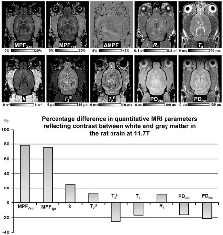
Example parametric maps of the rat brain obtained at the 11.7T: MPF maps reconstructed by the four-parameter fit of Z-spectroscopic images (MPFZsp) and single-point method (MPF1pt), their difference (ΔMPF), R1 map reconstructed from VFA data (R1), T2 map reconstructed from multi-echo data (T2), maps of the cross-relaxation rate constant (k) and T2 of the free and bound protons (T2F and T2B) obtained from the fit of Z-spectral data, and proton density maps reconstructed from VFA (PFvfa) and multi-echo (PDme) data. Greyscale range corresponds to the following parameter ranges: MPFZsp and MPF1pt: 0–20%. ΔMPF: −5 – +5%, R1: 0.1–0.8 s−1, T2: 0–70 ms, k: 0–5 s−1, T2B: 5–15 μsec. and T2F: 0–70 ms. PDvfa and PDme maps are presented in arbitrary units in the range from zero to the maximal voxel intensity of cerebrospinal fluid.
Figure 3.

Rat brain structures identified on the three coronal cross-sections (A, B, and C) of a 3D MPF map reconstructed by the single-point method. Abbreviations are as follows: OB, olfactory bulbs; Cg, cingulum; CC, corpus callosum; CPu, caudate putamen; ECap, left and right external capsule; ICap, internal capsule; F, fornix; SC, superior colliculus; IC, inferior colliculus; CWM, cerebellar white matter; CGM, cerebellar gray matter; Th, thalamus; H, hippocampus; Mc, motor cortex; Vc, visual cortex.
Table 1.
Relaxation and cross-relaxation parameters in WM and GM structures of the rat brain at 11.7T.
| Brain structure | R1, s−1 | T2, ms | k, s−1 | T2B, μs | T2F, ms | MPFZsp, % | MPF1pt, % | |
|---|---|---|---|---|---|---|---|---|
| Gray matter | olfactory bulb | 0.38±0.01 | 49.5±2.2 | 1.4±0.1 | 9.7±0.2 | 40.4±2.1 | 5.2 ±0.2 | 5.3±0.3 |
| caudate putamen | 0.45±0.01 | 36.6±1.5 | 1.8±0.1 | 10.2±0.3 | 33.9±2.6 | 6.2±0.3 | 6.8±0.6 | |
| hippocampus | 0.39±0.02 | 36.2±2.7 | 1.5±0.1 | 9.6±0.7 | 37.7±3.1 | 5.6±0.4 | 5.7±0.6 | |
| superior colliculus | 0.47±0.02 | 33.4±2.2 | 1.5±0.1 | 9.9±0.6 | 26.6±2.1 | 6.6±0.4 | 6.5±1.1 | |
| inferior colliculus | 0.44±0.03 | 31.6±1.9 | 1.9±0.3 | 10.1±0.5 | 28.2±4.8 | 5.9±0.5 | 6.4±0.7 | |
| cerebellar GM | 0.41±0.02 | 35.1±1.6 | 1.6±0.1 | 9.7±0.3 | 39.3±7.4 | 5.5±0.5 | 5.9±0.6 | |
| motor cortex | 0.37±0.01 | 44.7±2.9 | 1.7±0.3 | 9.4±0.2 | 34.9±8.1 | 5.4±0.3 | 5.7±0.6 | |
| visual cortex | 0.37±0.02 | 41.1±3.3 | 1.7±0.1 | 9.5±0.3 | 39.2±7.0 | 5.5±0.4 | 5.6±0.5 | |
| thalamus | 0.48±0.03 | 32.2±1.8 | 1.7±0.1 | 10.5±0.4 | 26.1±3.8 | 7.8±1.0 | 7.4±1.0 | |
| GM average | 0.42±0.02 | 37.8±2.2 | 1.6±0.2 | 9.8±0.4 | 34.0±4.5 | 5.9±0.4 | 6.1±0.7 | |
| White matter | cingulum | 0.45±0.0 | 31.3±2.1 | 2.2±0.3 | 10.7±0.4 | 29.6±5.0 | 9.2±0.6 | 9.4±1.0 |
| corpus callosum | 0.44±0.03 | 32.3±2.5 | 2.1±0.1 | 11.0±1.0 | 23.9±4.6 | 10.8±1.1 | 11.1±1.2 | |
| external capsule | 0.45±0.03 | 32.7±2.6 | 2.0±0.2 | 10.9±0.5 | 28.2±4.6 | 9.4±0.5 | 9.6±0.7 | |
| internal capsule | 0.52±0.03 | 28.1±3.2 | 2.0±0.2 | 11.2±0.6 | 20.4±2.9 | 13.3±1.4 | 12.8±0.9 | |
| fornix | 0.47±0.04 | 33.4±1.5 | 1.9±0.3 | 11.1±0.7 | 27.6±2.2 | 9.1±0.6 | 9.6±0.9 | |
| cerebellar WM | 0.47±0.0 | 31.0±1.8 | 2.1±0.1 | 11.6±0.8 | 22.9±2.0 | 12.1±0.9 | 12.1±1.3 | |
| WM average | 0.47±0.03 | 31.5±2.38 | 2.0±0.2 | 11.1±0.7 | 25.4±3.6 | 10.7±0.9 | 10.7±1.0 |
The bar graph of the percentage differences between average parameter values in WM and GM (calculated as 100(WM-GM)/GM) reflecting the capability of different parameters to generate brain tissue contrast is presented in Fig. 4. MPF maps reconstructed by both the full two-pool model parameter fit and the single-point method demonstrated high positive contrast between WM and GM allowing clear definition of anatomical structures (Figs. 2 and 3). Quantitatively, MPF enabled the largest difference between WM and GM being on the order of 75–80%, while other parameters showed relatively weak positive (k, R1, and T2B) or negative (T2F, T2, and PD) contrast with percentage differences not exceeding 25% (Fig. 4). Notably, R1 maps obtained at 11.7T demonstrated particularly weak positive contrast that was almost similar in absolute values to the negative contrast seen on the PDvfa maps (Figs. 2 and 4). This observation explains the loss of contrast between WM and GM on T1-weighted images in ultra-high fields, as the two above image contrast sources cancel each other. On the other hand, the synergistic effect of moderate negative WM-GM contrast provided by T2 and PD terms explains the typical high-contrast appearance of brain structures on routinely used in ultra-high fields T2-weighted images.
Figure 4.

Percentage difference between quantitative MRI parameters in WM and GM averaged across brain structures and reflecting tissue contrast on corresponding parametric maps.
MPF maps reconstructed by the four-parameter fit of Z-spectroscopic images and the single-point method (Fig. 2) demonstrated very similar visual appearance. Their difference image (Fig. 2) does not indicate any tissue-dependent patterns and shows only minor low-frequency variations, which may be associated with field instability during acquisition or sub-voxel motion propagation in the slab-selection direction. The Bland-Altman plot of MPF measurements pooled across animals and anatomic structures (Fig. 5a) indicates the absence of significant bias (mean difference = 0.14±0.68%, P=0.06) and systematic variations of the error. Excellent agreement between both methods was further confirmed by the regression analysis of mean MPF measurements in anatomic structures (Fig. 5b), which demonstrated strong correlation (Pearson’s correlation coefficient r=0.99, P<0.001) and non-significant intercept of the regression line (−0.4%, 95% confidence intervals: −1.0 – 0.2%, P=0.15).
Figure 5.

Agreement between MPF measurements obtained from maps reconstructed by the four-parameter fit of Z-spectroscopic images (MPFZsp) and single-point synthetic reference method (MPF1p): A: Bland-Altman plot of ROI measurements pooled across all animals and anatomic structures. Lines correspond to the mean difference (black) and limits of agreement (gray). B: Scatter plot of correlation between mean MPF measurements in brain structures with the regression line.
Figure 6 illustrates the application of fast MPF mapping for high-resolution 3D neuroanatomical imaging in ultra-high magnetic fields in vivo. In this example, extremely clear visualization of anatomical details was achieved with isotropic voxel size of 170 μm and an acceptable for high-resolution animal experiments total scan time of 1.5 hours. The full 3D dataset was submitted to the Data in Brief journal (Naumova et al., submitted).
Figure 6.

Reformatted orthogonal sections of a 3D MPF map of the rat brain obtained using the single-point synthetic-reference method with isotropic resolution of 170 μm.
4. Discussion
The key finding of this study is the evidence of the fact that MPF provides the highest brain tissue contrast in ultra-high magnetic fields, whereas other relaxation and cross-relaxation parameters have limited capabilities of image contrast generation. Opposed to lower fields, a small relative difference between T1 relaxation times in ultra-high fields precludes achieving sufficient contrast between WM and GM in T1-weighted imaging, as demonstrated by our results and earlier studies (de Graaf et al., 2006; van de Ven et al., 2007; Pohmann et al., 2011; Kara et al., 2013). Furthermore, a weak positive contrast based on R1 differences is offset by negative contrast due to differences in proton density, thus making impossible consistent visualization of tiny WM structures in the rodent brain using T1-weighted imaging. A simple fast single-point MPF mapping method (Yarnykh, 2016) fully exploits the benefits of MPF as a source of brain tissue contrast while enabling routine applications in ultra-high magnetic fields with a reasonable acquisition time, high spatial resolution, and robust reconstruction.
MPF values in WM and GM structures measured by both Z-spectroscopic and single-point techniques in this study are in excellent agreement with earlier animal data obtained at lower field strengths (Stanisz et al., 2005; Underhill et al., 2011; Samsonov et al., 2012). Particularly, in the normal rat brain in vivo (Underhill et al., 2011) at 3T, MPF were in the ranges 11.3–13.9% for WM and 5.7–7.3% for GM, which are very close to our data. Similar values were reported at 3T for fresh bovine brain tissues ex vivo (13.9% for WM and 5.0% for GM (Stanisz et al., 2005)) and canine brain in vivo (12.1% for WM and 5.4% for GM (Samsonov et al., 2012)). In ultra-high field of 16.4T (Pohmann et al., 2011), averaged MPF values across anatomic structures of the rat brain were also close to the values obtained in this study (10.8% in WM and 5.4% in GM). Our data appear in reasonable agreement with MPF measurements in the normal murine brain at 7T (Thiessen et al., 2013) (10% in the corpus callosum and 6.7% in cortex) and rat brain at 9.4T (Xu et al., 2014) (14.8% in WM and in 8.4% in GM as recalculated from the originally reported pool size ratio, a related measure of the macromolecular proton content), while slight positive or negative discrepancies can be attributed to distinctions in the measurement methodologies. MPF estimates in WM and GM of the human brain in vivo obtained at field strengths ranging from 0.5T to 7T based on multiple sources (Sled and Pike, 2001; Yarnykh, 2002; Ropele et al., 2003; Yarnykh and Yuan, 2004; Sled et al., 2004; Gloor et al., 2008; Underhill et al., 2009; Levesque et al., 2010; Dortch et al., 2011; Yarnykh, 2012; Dortch et al., 2013; Mossahebi et al., 2014; Petrie et al., 2014; Yarnykh et al., 2015a) are also close to our measurements. Taken together, these observations confirm independence of MPF of magnetic field strength. In view of the close association between MPF and myelin content established in a number of studies (Janve et al., 2013; Ou et al., 2009; Underhill et al., 2011; Samsonov et al., 2012; Thiessen et al., 2014), field independence of MPF is especially attractive in its applications as a myelin biomarker for both human and animal studies in contrast to relaxation-based techniques (MacKay et al., 1994; Deoni et al., 2008; Hwang et al., 2010; Glasser and Van Essen, 2011) where dependence of relaxation times on the field strength may bias or hamper estimation of the myelin content.
The values of the cross-relaxation rate constant reported in the literature are characterized by rather high variability. Our measurements appear in a reasonable agreement with reference 3T data for fresh bovine brain tissues ex vivo (Stanisz et al., 2005) where k values recalculated from the reverse rate constant R were 2.2 and 2.1 s−1 for WM and GM, respectively. There is also good correspondence between k measured in this study and data for the canine brain at 3T (2.5 s−1 in WM and 1.6 s−1 in GM (Samsonov et al., 2012)). Higher values in ranges of 1.9–3.7 s−1 and 2.2–3.8 s−1 for WM and GM, respectively were published for the rat brain at 3T (Underhill et al., 2011). Rodent studies at high and ultra-high field strengths reported somewhat lower than our estimates: 1.3 and 0.9 s−1 at 7T (Thiessen et al., 2013), 1.8 and 1.4 s−1 at 9.4T (Xu et al., 2014), and 1.7 and 1.5 s−1 at 16.4T (Pohmann et al., 2011) for WM and GM, respectively. Note that the above values for 16.4T (Pohmann et al., 2011) are based on recalculation from the reverse rate constant R after averaging across anatomic regions. Human data at field strengths of 0.5T and 1.5T (Sled and Pike, 2001; Yarnykh, 2002; Sled et al., 2004; Yarnykh and Yuan, 2004; Gloor et al., 2008; Levesque et al., 2010) demonstrated consistently higher k values (up to two-fold), especially in WM. At 3T, estimates of k in the human brain based on Z-spectroscopic measurements were close to our data for GM but about 30–50% higher in WM (Underhill et al., 2009; Mossahebi et al., 2014). Notably, k values at 3T corrected for the bias caused by the effect of cross-relaxation on R1 measurements (Mossahebi et al., 2014) appear in excellent quantitative agreement with our data for WM and slightly lower for GM. At the same time, the measurements by the on-resonance inversion recovery method (Dortch et al., 2011) at 3T yielded substantially lower k of 1.3 in WM and 1.1 s−1 in GM at 3T, as recalculated from the originally reported reverse rate constant. A similar approach at 7T (Dortch et al., 2013) resulted in higher and very close to each other k estimates in WM and GM of 2.5 and 2.6 s−1. It is also noticeable that visual appearance of k maps in this study suggests a reduced contrast between WM and GM compared to the published example maps of the human brain in lower fields (Sled and Pike, 2001; Yarnykh, 2002; Yarnykh and Yuan, 2004; Gloor et al., 2008; Underhill et al., 2009; Yarnykh, 2012; Mossahebi et al., 2014), though such inferences may be affected by differences in the noise level and window settings. Based on these observations, one cannot exclude a magnetic field dependence of the cross-relaxation rate constant with a trend of an overall decrease and a reduction of tissue-dependent variability in high fields, similar to R1. However, k is not theoretically expected to be field-dependent within the direct two-site magnetization exchange model, as the mechanisms contributing into this parameter, the nuclear Overhauser effect (NOE) and chemical exchange do not depend on magnetic field strength. Particularly, NOE in high fields at the slow molecular motion limit is dominated by the field-independent zero-quantum term with a negligible contribution from two-quantum transitions (Edzes and Samulski, 1978). Some spurious field effects on k may arise from the simplified nature of the pseudo-first order two-pool model and certain assumptions about R1 of pools in Z-spectroscopic data processing. Specifically, field-dependent changes in R1 of intermediate exchange pools not accounted in the two-pool model may affect k as an effective rate constant defined within this model. Dependence of the cross-relaxation rate constant on R1 of extracellular water originating from the two-pool approximation of the three- and four-pool exchange models has recently been demonstrated by simulations (Li et al., 2016). Depending on the water compartmentalization scheme and a measurement technique, the trends of both decrease and increase of the measured rate constant with an increase of R1 were predicted (Li et al., 2016). As such, multi-compartment exchange and cross-relaxation may theoretically explain possible field dependence of k or R via changes in R1 of pools. Another source of field-dependent variability of the cross-relaxation rate constant may originate from the dipolar order effect (Morrison et al., 1995; Swanson et al., 2016; Varma et al., 2015b) neglected in the standard two-pool model. Previous studies have demonstrated that inclusion of the dipolar order reservoir into the two-pool model affects cross-relaxation rates (Morrison et al., 1995; Varma et al., 2015b), and the time constant describing dipolar order relaxation, T1D may be field-dependent (Varma et al., 2015b; Varma et al., 2016). Field dependence of R1 of the bound pool may also propagate into the measured k values, if the assumption about equality of R1 of the pools used in the processing algorithm (Yarnykh, 2012) is violated, as suggested by some studies (Helms and Hagberg, 2009; Pohmann et al., 2011; van Gelderen et al., 2016). Finally, a slight dependence of k on magnetic field through observed R1 may be caused by the bias due to the unaccounted effect of cross-relaxation on VFA R1 measurements (Mossahebi et al., 2014), though correction for this bias would result in further reduction of k (Mossahebi et al., 2014). However, given high uncertainties associated with k and R estimation (Portnoy and Stanisz, 2007; Yarnykh, 2012), it is impossible to conclude at this point, whether cross-relaxation rate constants are really field-dependent. It also should be pointed out that relatively high k values were obtained on human MRI scanners with the use of off-resonance saturation techniques under specific absorption rate restrictions, which might adversely affect accuracy of k values due to insufficient saturation power (Yarnykh, 2012).
T2B measurements obtained in this study are highly consistent with the literature data based on the analysis with the Super-Lorentzian lineshape (Morrison and Henkelman, 1995; Sled and Pike, 2001; Yarnykh, 2002; Sled et al., 2004; Stanisz et al, 2005; Underhill et al., 2009; Levesque et al., 2010; Pohmann et al., 2011; Underhill et al., 2011; Samsonov et al., 2012; Yarnykh, 2012; Thiessen et al., 2013; Mossahebi et al., 2014; Pampel et al., 2015; Varma et al., 2015b) and do not suggest any field dependence of this parameter. Generally, T2B values demonstrate minimal distinctions between WM and GM and a narrow range of variations (typically about 8–12 μs) in the brain. Residual tissue contrast on T2B maps has been recently attributed to the directional dependence of this parameter in WM (Yarnykh, 2012; Pampel et al., 2015). The visual appearance of T2B maps of the rat brain at 11.7T (Fig. 2) is in agreement with this finding, as slightly higher T2B values are observed in WM regions comprising fiber tracts that are known (Figini et al., 2015; Jugé et al., 2016) to run approximately parallel to the direction of the main magnetic field vector (rostral-caudal direction in Fig. 2).
Comparison of T2 relaxation times determined from multiple spin-echoes and T2F measured by Z-spectroscopy in this study demonstrates close agreement between these parameters with T2F only slightly shorter than T2. This finding contradicts to earlier reports for lower magnetic fields (1.5T and 3T) (Sled and Pike, 2001; Underhill et al., 2009; Levesque et al., 2010; Underhill et al., 2011) where T2F were approximately two-fold shorter than T2 at corresponding field strengths. At the same time, T2 and T2F appeared almost identical at 7T (Thiessen et al., 2013). Quantitative comparison of T2F values measured in this study with the literature (Sled and Pike, 2001; Underhill et al., 2009; Levesque et al., 2010; Underhill et al., 2011; Thiessen et al., 2013) may suggest minor magnetic field dependence for this parameter, although existing data are insufficient to substantiate this conclusion in view of different model assumptions underlying Z-spectra analysis in the above publications. Particularly, T2F in ranges 30–40 ms for WM and 50–55 ms for GM were reported for the human brain at 1.5T (Sled and Pike, 2001; Levesque et al., 2010). At 3T, T2F in the rat brain were in ranges of 27–33 ms in WM and 41–55 in GM (Underhill et al., 2011), whereas shorter values were reported for the human brain (17–27 ms in WM and 29–49 in GM (Underhill et al., 2009)). However, relatively long values of 39 and 45 ms for the corpus callosum and cortex, respectively, were found in the murine brain at 7T (Thiessen et al., 2013). As such, apparent convergence of T2 and T2F values in ultra-high fields is mainly caused by shortening of the observed T2 with an increase of the field strength, which has been noted in numerous studies (Michaeli et al., 2002; de Graaf et al., 2006; Pohmann et al., 2011; Kara et al., 2013) and appears in excellent agreement with our T2 measurements at 11.7T. Observed trends in field-dependent discrepancies between T2 and T2F support the earlier explanation (Sled and Pike, 2001) of T2F behavior in terms of the weighted average of multiple T2 components corresponding to several water pools and the diffusion-mediated mechanism of T2 shortening in high magnetic fields (Michaeli et al., 2002). Specifically, T2F values measured by Z-spectroscopic techniques reflect the presence of water pools with restricted mobility characterized by short T2, which participate in the magnetization exchange with macromolecular protons and are treated collectively with free water as the free pool in the two-pool model. These short-T2 proton populations typically belong to water immobilized within lipid bilayers of plasma membranes and/or on protein surfaces. Accordingly, they are characterized by much slower diffusion compared to free water, thus being much less affected by the dynamic dephasing on microscopic susceptibility gradients that has been suggested as the main reason for shortening of the observed T2 in ultra-high fields (Michaeli et al., 2002). Of note, a similar mechanism was proposed to explain discrepancies in magnetic field dependences of T2 of spectral signals of water, metabolites, and macromolecules (de Graaf et al., 2006).
Results of this study provide validation of the fast single-point MPF mapping method with synthetic reference image (Yarnykh, 2012) for animal brain applications in ultra-high magnetic fields. This method enables the fastest possible generation of MPF maps and can be implemented with very high spatial resolution and a reasonable scan time. MPF maps obtained with the single-point method appear in excellent agreement with those reconstructed by the full fit of the two-pool model parameters. This result is similar to the findings of the earlier study (Yarnykh, 2012) where fast single-point MPF mapping was extensively validated for human brain imaging on a clinical 3T MRI scanner. Additionally, our results provide direct validation of a more time-efficient variant of the single-point method based on synthetic reference reconstruction, which has not been compared with Z-spectroscopic measurements in the initial publication (Yarnykh, 2016). The implementation of fast MPF mapping in ultra-high fields is very similar to that previously described at 3T (Yarnykh, 2012; Yarnykh, 2016), except for the constrained value of the product R1T2F for brain tissues, which demonstrated apparent field dependence. The value of R1T2F = 0.013 appears about two-fold smaller than that for 3T (R1T2F = 0.022 (Yarnykh, 2012)) mainly due to a decrease of R1. Based on the known field-dependence of R1 (Bottomley et al., 1984; Rooney et al., 2007), the value of the product R1T2F can be easily estimated for implementations of the single-point reconstruction algorithm at different field strengths. The constrained value of the reverse rate constant R determined in this study (23 s−1) slightly differs from that at 3T (19 s−1 (Yarnykh, 2012)). However, in view of large uncertainties in determination of this parameter (Portnoy and Stanisz, 2007) and low sensitivity of the signal to R at low saturation rates (Yarnykh, 2012), this difference is practically negligible, and some rounded value (for example, 20 s−1) can be used as a standard constant for the single-point brain MPF mapping algorithm in a range of field strengths. Finally, due to field independence of T2B confirmed in this study, the standard whole-brain value of 10 μs can be used for any magnetic field.
The findings of this study may be helpful for the interpretation of contrast properties of parametric maps generated using recent semi-quantitative MT techniques, such as MTsat (Helms et al., 2008) and ihMTR (Varma et al., 2015a). Since MPF appears the main two-pool model parameter determining high-field brain tissue contrast, these techniques can be viewed as different ways to probe MPF. At the same time, effects of other two-pool model parameters may be synergistic, thus enabling additional contrast features. Particularly, a reduced inhomogeneous MT signal in muscle has been attributed to a much shorter, as compared to brain tissues, dipolar relaxation time T1D (Varma et al., 2015b; Varma et al., 2016). However, this parameter appears similar in WM and GM (Varma et al., 2016) and, therefore, is unlikely to significantly contribute into the observed contrast between brain tissues. In the practical aspect, the common feature of the MTsat, ihMTR, and fast MPF mapping methods is that all of them require three source images to reconstruct corresponding maps and are capable of generating high neuroanatomical contrast in both low and high magnetic fields. An important advantage of MPF mapping is the capability of absolute quantitation, while other techniques may benefit from simpler image processing. More research is needed to directly compare the above methods in the context of time efficiency, available spatial resolution, and image quality in structural neuroimaging applications.
This study demonstrates that fast 3D MPF mapping provides a useful approach for neuroanatomical applications in ultra-high fields where its contrast-generation capability enables excellent visualization of WM and GM structures based on differences in their myelination. An additional advantage of MPF mapping in both quantitative and structural imaging applications is its insensitivity to the presence paramagnetic ions including iron (Yarnykh, 2016). It has been demonstrated that MPF mapping improves visualization of iron-rich GM anatomical structures as compared to T1-weighted imaging or R1-mapping (Yarnykh, 2016) and enables unbiased iron-insensitive characterization of demyelination in subcortical GM nuclei (Krutenkova et al., 2015). Due to an increased sensitivity of high-field imaging to magnetic susceptibility effects, this feature of MPF mapping may become especially important for any high-field applications related to quantitative assessment of myelination. Another promising area of applications of high-resolution MPF mapping might include generation of anatomical templates in cell labeling and tracking studies. Most of the MRI cell-tracking techniques employ iron-oxide super-paramagnetic particles for cell labeling (Bulte et al., 2004; Lepore et al., 2006). Routinely used for neuroanatomical visualization in high fields T2-weighted imaging is highly sensitive to the signal void effect caused by super-paramagnetic substances as well as the presence of hemorrhage after surgical procedures, which may obscure anatomical details in cell labeling applications. Since MPF mapping is based on fast gradient-echo acquisition, the signal void effect for such applications can be reduced by implementing protocols with ultra-short echo time. In combination with inherent insensitivity of MPF to the presence of paramagnetic materials, MPF mapping with ultra-short TE acquisition may become a method of choice for detailed imaging of brain anatomy before and after cell transplantation.
5. Conclusion
This study demonstrates that MPF enables the highest contrast between WM and GM in ultra-high magnetic fields as compared to other relaxation and cross-relaxation parameters. The contrast-generating capability of MPF can be exploited using the fast and robust method for 3D mapping of this parameter based on three source images, which provides a combined neuroimaging approach for both high-resolution structural imaging and quantitative tissue characterization.
Supplementary Material
Highlights.
Macromolecular proton fraction (MPF) mapping was used to image rat brain at 11.7T.
MPF provided the effective source of ultra-high-field brain tissue contrast.
Fast single-point MPF mapping method was validated for high-field MRI applications.
MPF mapping enables high-resolution and high-contrast imaging of brain anatomy.
Acknowledgments
The authors acknowledge financial support from the Russian Science Foundation (project No14-45-00040) for experimental studies, data analysis, and manuscript preparation and National Institutes of Health (grant R21EB016135) for software development. Animal procedures were carried out at the Center for Genetic Resources of Laboratory Animals at the Institute of Cytology and Genetics (Siberian Branch, Russian Academy of Sciences) operating under support of the Ministry of Education and Science projects RFMEFI61914X0005 and RFMEFI62114X0010.
Abbreviations
- MPF
macromolecular proton fraction
- MPFZsp
MPF maps reconstructed by the four-parameter fit of Z-spectroscopic images
- MPF1pt
MPF single-point method
- MRI
magnetic resonance imaging
- T
Tesla
- 3D
three dimensional
- MT
magnetization transfer
- MTR
MT ratio
- MTsat
MT saturation
- ihMTR
inhomogeneous MTR
- PD
proton density
- SNR
signal-to-noise ratio
- RARE
rapid acquisition with relaxation enhancement
- FSE
fast spin echo
- GRE
gradient echo
- TR
repetition time
- TE
echo time
- FOV
field of view
- WM
white matter
- GM
gray matter
- VFA
variable flip angle
- AFI
actual flip-angle imaging
- ME
multi-echo
- Δ
offset frequencies
- ROI
region of interest
- T1D
dipolar order longitudinal relaxation time
- T2F
T2 of free protons
- T2B
T2 of bound protons
- OB
olfactory bulbs
- Cg
cingulum
- CC
corpus callosum
- CPu
caudate putamen
- ECap
left and right external capsule
- ICap
internal capsule
- F
fornix
- SC
superior colliculus
- IC
inferior colliculus
- CWM
cerebellar white matter
- CGM
cerebellar gray matter
- Th
thalamus
- H
hippocampus
- Mc
motor cortex
- Vc
visual cortex
Footnotes
Publisher's Disclaimer: This is a PDF file of an unedited manuscript that has been accepted for publication. As a service to our customers we are providing this early version of the manuscript. The manuscript will undergo copyediting, typesetting, and review of the resulting proof before it is published in its final citable form. Please note that during the production process errors may be discovered which could affect the content, and all legal disclaimers that apply to the journal pertain.
References
- Balchandani P, Naidich TP. Ultra-High-Field MR Neuroimaging. Am J Neuroradiol. 2015;36:1204–1215. doi: 10.3174/ajnr.A4180. [DOI] [PMC free article] [PubMed] [Google Scholar]
- Boretius S, Dechent P, Frahm J, Helms G. Magnetization Transfer Mapping of Myelinated Fiber Tracts in Living Mice at 9.4 T. Proc Intl Soc Mag Reson Med. 2010:690. [Google Scholar]
- Bottomley PA, Foster TH, Argersinger RE, Pfeifer LM. A review of normal tissue hydrogen NMR relaxation times and relaxation mechanisms from 1–100 MHz: dependence on tissue type, NMR frequency, temperature, species, excision, and age. Med Phys. 1984;11:425–448. doi: 10.1118/1.595535. [DOI] [PubMed] [Google Scholar]
- Bulte JW, Arbab AS, Douglas T, Frank JA. Preparation of Magnetically Labeled Cells for Cell Tracking by Magnetic Resonance Imaging. Methods Enzymol. 2004;386:275–299. doi: 10.1016/S0076-6879(04)86013-0. [DOI] [PubMed] [Google Scholar]
- de Graaf RA, Brown PB, McIntyre S, Nixon TW, Behar KL, Rothman DL. High magnetic field water and metabolite proton T1 and T2 relaxation in rat brain in vivo. Magn Reson Med. 2006;56:386–394. doi: 10.1002/mrm.20946. [DOI] [PubMed] [Google Scholar]
- Deoni SCL, Rutt BK, Arun T, Pierpaoli C, Jones DK. Gleaning multicomponent T1 and T2 information from steady-state imaging data. Magn Reson Med. 2008;60:1372–1387. doi: 10.1002/mrm.21704. [DOI] [PubMed] [Google Scholar]
- Dortch RD, Li K, Gochberg DF, Welch EB, Dula AN, Tamhane AA, Gore JC, Smith SA. Quantitative magnetization transfer imaging in human brain at 3 T via selective inversion recovery. Magn Reson Med. 2011;66:1346–1352. doi: 10.1002/mrm.22928. [DOI] [PMC free article] [PubMed] [Google Scholar]
- Dortch RD, Moore J, Li K, Jankiewicz M, Gochberg DF, Hirtle JA, Gore JC, Smith SA. Quantitative magnetization transfer imaging of human brain at 7 T. Neuroimage. 2013;64:640–649. doi: 10.1016/j.neuroimage.2012.08.047. [DOI] [PMC free article] [PubMed] [Google Scholar]
- Dousset V, Grossman RI, Ramer KN, Schnall MD, Young LH, Gonzalez-Scarano F, Lavi E, Cohen JA. Experimental allergic encephalomyelitis and multiple sclerosis: lesion characterization with magnetization transfer imaging. Radiology. 1992;182:483–491. doi: 10.1148/radiology.182.2.1732968. [DOI] [PubMed] [Google Scholar]
- Edzes HT, Samulski ET. The measurement of cross-relaxation effects in the proton NMR spin-lattice relaxation of water in biological systems: hydrated collagen and muscle. J Magn Reson. 1978;31:207–229. [Google Scholar]
- Figini M, Zucca I, Aquino D, Pennacchio P, Nava S, Di Marzio A, Preti MG, Baselli G, Spreafico R, Frassoni C. In vivo DTI tractography of the rat brain: an atlas of the main tracts in Paxinos space with histological comparison. Magn Reson Imaging. 2015;33:296–303. doi: 10.1016/j.mri.2014.11.001. [DOI] [PubMed] [Google Scholar]
- Glasser MF, Van Essen DC. Mapping human cortical areas in vivo based on myelin content as revealed by T1- and T2-weighted MRI. J Neurosci. 2011;31:11597–11616. doi: 10.1523/JNEUROSCI.2180-11.2011. [DOI] [PMC free article] [PubMed] [Google Scholar]
- Gloor M, Scheffler K, Bieri O. Quantitative magnetization transfer imaging using balanced SSFP. Magn Reson Med. 2008;60:691–700. doi: 10.1002/mrm.21705. [DOI] [PubMed] [Google Scholar]
- Helms G, Hagberg GE. In vivo quantification of the bound pool T1 in human white matter using the binary spin-bath model of progressive magnetization transfer saturation. Phys Med Biol. 2009;54:N529–540. doi: 10.1088/0031-9155/54/23/N01. [DOI] [PubMed] [Google Scholar]
- Helms G, Dathe H, Kallenberg K, Dechent P. High-resolution maps of magnetization transfer with inherent correction for RF inhomogeneity and T1 relaxation obtained from 3D FLASH MRI. Magn Reson Med 2008. 2008;60:1396–1407. doi: 10.1002/mrm.21732. [DOI] [PubMed] [Google Scholar]
- Hwang D, Kim DH, Du YP. In vivo multi-slice mapping of myelin water content using T2* decay. Neuroimage. 2010;52:198–204. doi: 10.1016/j.neuroimage.2010.04.023. [DOI] [PubMed] [Google Scholar]
- Jugé L, Pong AC, Bongers A, Sinkus R, Bilston LE, Cheng S. Changes in Rat Brain Tissue Microstructure and Stiffness during the Development of Experimental Obstructive Hydrocephalus. PLoS One. 2016;11:e0148652. doi: 10.1371/journal.pone.0148652. [DOI] [PMC free article] [PubMed] [Google Scholar]
- Janve VA, Zu Z, Yao SY, Li K, Zhang FL, Wilson KJ, Ou X, Does MD, Subramaniam S, Gochberg DF. The radial diffusivity and magnetization transfer pool size ratio are sensitive markers for demyelination in a rat model of type III multiple sclerosis (MS) lesions. Neuroimage. 2013;74:298–305. doi: 10.1016/j.neuroimage.2013.02.034. [DOI] [PMC free article] [PubMed] [Google Scholar]
- Kara F, Chen F, Ronen I, de Groot HJ, Matysik J, Alia A. In vivo measurement of transverse relaxation time in the mouse brain at 17.6 T. Magn Reson Med. 2013;70:985–993. doi: 10.1002/mrm.24533. [DOI] [PubMed] [Google Scholar]
- Krutenkova EP, Khodanovich M Yu, Bowen JD, Gangadharan B, Jung Henson LK, Mayadev A, Repovic P, Qian P, Yarnykh VL. Demyelination and iron accumulation in subcortical gray matter (GM) in multiple sclerosis (MS) Ann Neurol. 2015;78:S65–S65. [Google Scholar]
- Lepore AC, Walczak P, Rao MS, Fischer I, Bulte JW. MR imaging of lineage-restricted neural precursors following transplantation into the adult spinal cord. Exp Neurol. 2006;201:49–59. doi: 10.1016/j.expneurol.2006.03.032. [DOI] [PubMed] [Google Scholar]
- Levesque IR, Sled JG, Narayanan S, Giacomini PS, Ribeiro LT, Arnold DL, Pike GB. Reproducibility of quantitative magnetization-transfer imaging parameters from repeated measurements. Magn Reson Med. 2010;64:391–400. doi: 10.1002/mrm.22350. [DOI] [PubMed] [Google Scholar]
- Li K, Li H, Zhang XY, Stokes AM, Jiang X, Kang H, Quarles CC, Zu Z, Gochberg DF, Gore JC, Xu J. Influence of water compartmentation and heterogeneous relaxation on quantitative magnetization transfer imaging in rodent brain tumors. Magn Reson Med. 2016;76:635–644. doi: 10.1002/mrm.25893. [DOI] [PMC free article] [PubMed] [Google Scholar]
- Lövblad KO, Haller S, Pereira VM. Stroke: high-field magnetic resonance imaging. Neuroimaging Clin N Am. 2012;22:191–205. doi: 10.1016/j.nic.2012.02.002. [DOI] [PubMed] [Google Scholar]
- MacKay A, Whittall K, Mädler J, Li D, Paty D, Graeb D. In vivo visualization of myelin water in brain by magnetic resonance. Magn Reson Med. 1994;31:673–677. doi: 10.1002/mrm.1910310614. [DOI] [PubMed] [Google Scholar]
- Michaeli S, Garwood M, Zhu XH, DelaBarre L, Andersen P, Adriany G, Merkle H, Ugurbil K, Chen W. Proton T2 relaxation study of water, N-acetylaspartate, and creatine in human brain using Hahn and Carr-Purcell spin echoes at 4T and 7T. Magn Reson Med. 2002;47:629–633. doi: 10.1002/mrm.10135. [DOI] [PubMed] [Google Scholar]
- Morrison C, Henkelman RM. A model for magnetization transfer in tissues. Magn Reson Med. 1995;33:475–482. doi: 10.1002/mrm.1910330404. [DOI] [PubMed] [Google Scholar]
- Mossahebi P, Yarnykh VL, Samsonov A. Analysis and correction of biases in cross-relaxation MRI due to biexponential longitudinal relaxation. Magn Reson Med. 2014;71:830–838. doi: 10.1002/mrm.24677. [DOI] [PMC free article] [PubMed] [Google Scholar]
- Morrison C, Stanisz G, Henkelman RM. Modeling magnetization transfer for biological-like systems using a semi-solid pool with a super-Lorentzian lineshape and dipolar reservoir. J Magn Reson Ser B. 1995;108:103–113. doi: 10.1006/jmrb.1995.1111. [DOI] [PubMed] [Google Scholar]
- Naumova AV, Akulov AE, Khodanovich M Yu, Yarnykh VL. High-resolution three-dimensional quantitative map of the macromolecular proton fraction distribution in the normal rat brain. Data Brief. doi: 10.1016/j.dib.2016.11.066. (submitted) [DOI] [PMC free article] [PubMed] [Google Scholar]
- Ou X, Sun SW, Liang HF, Song SK, Gochberg DF. The MT pool size ratio and the DTI radial diffusivity may reflect the myelination in shiverer and control mice. NMR Biomed. 2009;22:480–487. doi: 10.1002/nbm.1358. [DOI] [PMC free article] [PubMed] [Google Scholar]
- Pampel A, Müller DK, Anwander A, Marschner H, Möller HE. Orientation dependence of magnetization transfer parameters in human white matter. Neuroimage. 2015;114:136–146. doi: 10.1016/j.neuroimage.2015.03.068. [DOI] [PubMed] [Google Scholar]
- Petrie EC, Cross DJ, Yarnykh VL, Richards T, Martin NM, Pagulayan K, Hoff D, Hart K, Mayer C, Tarabochia M, Raskind MA, Minoshima S, Peskind ER. Neuroimaging, behavioral, and psychological sequelae of repetitive combined blast/impact mild traumatic brain injury in Iraq and Afghanistan war veterans. J Neurotrauma. 2014;31:425–436. doi: 10.1089/neu.2013.2952. [DOI] [PMC free article] [PubMed] [Google Scholar]
- Prevost VH, Girard OM, Varma G, Alsop DC, Duhamel G. Minimizing the effects of magnetization transfer asymmetry on inhomogeneous magnetization transfer (ihMT) at ultra-high magnetic field (11.75 T) MAGMA. 2016;29:699–709. doi: 10.1007/s10334-015-0523-2. [DOI] [PubMed] [Google Scholar]
- Pohmann R, Shajan G, Balla DZ. Contrast at high field: relaxation times, magnetization transfer and phase in the rat brain at 16.4 T. Magn Reson Med. 2011;66:1572–1581. doi: 10.1002/mrm.22949. [DOI] [PubMed] [Google Scholar]
- Portnoy S, Stanisz GJ. Modeling pulsed magnetization transfer. Magn Reson Med. 2007;58:144–155. doi: 10.1002/mrm.21244. [DOI] [PubMed] [Google Scholar]
- Ropele S, Seifert T, Enzinger C, Fazekas F. Method for quantitative imaging of the macromolecular 1H fraction in tissues. Magn Reson Med. 2003;49:864–871. doi: 10.1002/mrm.10427. [DOI] [PubMed] [Google Scholar]
- Raya JG, Dietrich O, Horng A, Weber J, Reiser MF, Glaser C. T2 measurement in articular cartilage: impact of the fitting method on accuracy and precision at low SNR. Magn Reson Med. 2010;63:181–193. doi: 10.1002/mrm.22178. [DOI] [PubMed] [Google Scholar]
- Rooney WD, Johnson G, Li X, Cohen ER, Kim SG, Ugurbil K, Springer CS., Jr Magnetic field and tissue dependencies of human brain longitudinal 1H2O relaxation in vivo. Magn Reson Med. 2007;57:308–318. doi: 10.1002/mrm.21122. [DOI] [PubMed] [Google Scholar]
- Samsonov A, Alexander AL, Mossahebi P, Wu YC, Duncan ID, Field AS. Quantitative MR imaging of two-pool magnetization transfer model parameters in myelin mutant shaking pup. Neuroimage. 2012;62:1390–1398. doi: 10.1016/j.neuroimage.2012.05.077. [DOI] [PMC free article] [PubMed] [Google Scholar]
- Skinner TE, Glover GH. An extended two-point Dixon algorithm for calculating separate water, fat, and B0 images. Magn Reson Med. 1997;37:628–630. doi: 10.1002/mrm.1910370426. [DOI] [PubMed] [Google Scholar]
- Sled JG, Levesque I, Santos AC, Francis SJ, Narayanan S, Brass SD, Arnold DL, Pike GB. Regional variations in normal brain shown by quantitative magnetization transfer imaging. Magn Reson Med. 2004;51:299–303. doi: 10.1002/mrm.10701. [DOI] [PubMed] [Google Scholar]
- Sled JG, Pike GB. Quantitative imaging of magnetization transfer exchange and relaxation properties in vivo using MRI. Magn Reson Med. 2001;46:923–931. doi: 10.1002/mrm.1278. [DOI] [PubMed] [Google Scholar]
- Stanisz GJ, Odrobina EE, Pun J, Escaravage M, Graham SJ, Bronskill MJ, Henkelman RM. T1, T2 relaxation and magnetization transfer in tissue at 3T\ Magn Reson Med. 2005;54:507–512. doi: 10.1002/mrm.20605. [DOI] [PubMed] [Google Scholar]
- Swanson SD, Malyarenko DI, Fabiilli ML, Welsh RC, Nielsen J-F, Srinivasan A. Molecular, dynamic, and structural origin of inhomogeneous magnetization transferin lipid membranes. Magn Reson Med. 2016 doi: 10.1002/mrm.26210. Epub ahead of print. [DOI] [PubMed] [Google Scholar]
- Thiessen JD, Zhang Y, Zhang H, Wang L, Buist R, Del Bigio MR, Kong J, Li XM, Martin M. Quantitative MRI and ultrastructural examination of the cuprizone mouse model of demyelination. NMR Biomed. 2013;26:1562–1581. doi: 10.1002/nbm.2992. [DOI] [PubMed] [Google Scholar]
- Ugurbil K. Magnetic resonance imaging at ultrahigh fields. IEEE Trans Biomed Eng. 2014;61:1364–1379. doi: 10.1109/TBME.2014.2313619. [DOI] [PMC free article] [PubMed] [Google Scholar]
- Underhill HR, Rostomily RC, Mikheev AM, Yuan C, Yarnykh VL. Fast bound pool fraction imaging of the in vivo rat brain: association with myelin content and validation in the C6 glioma model. Neuroimage. 2011;54:2052–2065. doi: 10.1016/j.neuroimage.2010.10.065. [DOI] [PMC free article] [PubMed] [Google Scholar]
- Underhill HR, Yuan C, Yarnykh VL. Direct quantitative comparison between cross-relaxation imaging and diffusion tensor imaging of the human brain at 3.0 T. Neuroimage. 2009;47:1568–1578. doi: 10.1016/j.neuroimage.2009.05.075. [DOI] [PubMed] [Google Scholar]
- van Gelderen P, Jiang X, Duyn JH. Effects of magnetization transfer on T1 contrast in human brain white matter. Neuroimage. 2016;128:85–95. doi: 10.1016/j.neuroimage.2015.12.032. [DOI] [PMC free article] [PubMed] [Google Scholar]
- van de Ven RC, Hogers B, van den Maagdenberg AM, de Groot HJ, Ferrari MD, Frants RR, Poelmann RE, van der Weerd L, Kiihne SR. T(1) relaxation in in vivo mouse brain at ultra-high field. Magn Reson Med. 2007;58:390–395. doi: 10.1002/mrm.21313. [DOI] [PubMed] [Google Scholar]
- Varma G, Duhamel G, de Bazelaire C, Alsop DC. Magnetization transfer from inhomogeneously broadened lines: A potential marker for myelin. Magn Reson Med. 2015a;73:614–622. doi: 10.1002/mrm.25174. [DOI] [PMC free article] [PubMed] [Google Scholar]
- Varma G, Girard OM, Prevost VH, Grant AK, Duhamel G, Alsop DC. Interpretation of magnetization transfer from inhomogeneously broadened lines (ihMT) in tissues as a dipolar order effect within motion restricted molecules. J Magn Reson. 2015b;260:67–76. doi: 10.1016/j.jmr.2015.08.024. [DOI] [PubMed] [Google Scholar]
- Varma G, Girard OM, Prevost VH, Grant A, Duhamel GD, Alsop DC. In vivo measurement of a new source of tissue contrast, the dipolar relaxation time, T1D, using a modified ihMT sequence. Proc Intl Soc Mag Reson Med. 2016:802. doi: 10.1002/mrm.26523. [DOI] [PubMed] [Google Scholar]
- Xu J, Li K, Zu Z, Li X, Gochberg DF, Gore JC. Quantitative magnetization transfer imaging of rodent glioma using selective inversion recovery. NMR Biomed. 2014;27:253–260. doi: 10.1002/nbm.3058. [DOI] [PMC free article] [PubMed] [Google Scholar]
- Yarnykh VL. Pulsed Z-spectroscopic imaging of cross-relaxation parameters in tissues for human MRI: theory and clinical applications. Magn Reson Med. 2002;47:929–939. doi: 10.1002/mrm.10120. [DOI] [PubMed] [Google Scholar]
- Yarnykh VL, Yuan C. Cross-relaxation imaging reveals detailed anatomy of white matter fiber tracts in the human brain. Neuroimage. 2004;23:409–424. doi: 10.1016/j.neuroimage.2004.04.029. [DOI] [PubMed] [Google Scholar]
- Yarnykh VL. Actual flip-angle imaging in the pulsed steady state: a method for rapid three-dimensional mapping of the transmitted radiofrequency field. Magn Reson Med. 2007;57:192–200. doi: 10.1002/mrm.21120. [DOI] [PubMed] [Google Scholar]
- Yarnykh VL. Fast macromolecular proton fraction mapping from a single off-resonance magnetization transfer measurement. Magn Reson Med. 2012;68:166–178. doi: 10.1002/mrm.23224. [DOI] [PMC free article] [PubMed] [Google Scholar]
- Yarnykh VL. Time-efficient, high-resolution, whole brain three-dimensional macromolecular proton fraction mapping. Magn Reson Med. 2016;75:2100–2106. doi: 10.1002/mrm.25811. [DOI] [PMC free article] [PubMed] [Google Scholar]
- Yarnykh VL, Bowen JD, Samsonov A, Repovic P, Mayadev A, Qian P, Gangadharan B, Keogh BP, Maravilla KR, Jung Henson LK. Fast whole-brain three-dimensional macromolecular proton fraction mapping in multiple sclerosis. Radiology. 2015a;274:210–220. doi: 10.1148/radiol.14140528. [DOI] [PMC free article] [PubMed] [Google Scholar]
- Yarnykh VL, Tartaglione EV, Ioannou GN. Fast macromolecular proton fraction mapping of the human liver in vivo for quantitative assessment of hepatic fibrosis. NMR Biomed. 2015b;28:1716–1725. doi: 10.1002/nbm.3437. [DOI] [PMC free article] [PubMed] [Google Scholar]
Associated Data
This section collects any data citations, data availability statements, or supplementary materials included in this article.