Nuisance Regression of High-Frequency Functional Magnetic Resonance Imaging Data: Denoising Can Be Noisy

Abstract

Recently, emerging studies have demonstrated the existence of brain resting-state spontaneous activity at frequencies higher than the conventional 0.1 Hz. A few groups utilizing accelerated acquisitions have reported persisting signals beyond 1 Hz, which seems too high to be accommodated by the sluggish hemodynamic process underpinning blood oxygen level-dependent contrasts (the upper limit of the canonical model is ∼0.3 Hz). It is thus questionable whether the observed high-frequency (HF) functional connectivity originates from alternative mechanisms (e.g., inflow effects, proton density changes in or near activated neural tissue) or rather is artificially introduced by improper preprocessing operations. In this study, we examined the influence of a common preprocessing step—whole-band linear nuisance regression (WB-LNR)—on resting-state functional connectivity (RSFC) and demonstrated through both simulation and analysis of real dataset that WB-LNR can introduce spurious network structures into the HF bands of functional magnetic resonance imaging (fMRI) signals. Findings of present study call into question whether published observations on HF-RSFC are partly attributable to improper data preprocessing instead of actual neural activities.

Introduction

Permitted by recent technical advances in magnetic resonance (MR) acquisition that provide accelerated temporal sampling rates, there has been growing interest in exploiting brain resting-state functional connectivity (RSFC) at frequencies beyond the conventional 0.1 Hz. These early investigations (Boubela et al., 2013; Boyacioglu et al., 2013; Chen and Glover, 2015; Gohel and Biswal, 2015; Lee et al., 2013; Lin et al., 2015; Niazy et al., 2011; Wu et al., 2008), although with disparate acquisition protocols, converge on similar conclusions that spontaneous activity persists at frequencies well above the typical upper limit of 0.1 Hz and shares partially overlapped functional information across frequencies. These intriguing findings have offered new biomarker opportunities for clinical and neuroscience research and have provoked emerging efforts to reexamine the frequency dependence of brain functional behaviors across broad mental states (Lin et al., 2015; Yuan et al., 2014), age (Smith-Collins et al., 2015), and clinical populations (Morgan et al., 2015; Sours et al., 2015; Wang et al., 2015).

The potential concern with these promising high-frequency (HF) network connectivity results is that the blood oxygenation level-dependent (BOLD) mechanism tracks neural activity in an indirect and very sluggish manner, which naturally confers an upper limit on the neural information's observable frequencies. Previously, we demonstrated BOLD-like components up to 0.5 Hz and simulated the RS hemodynamic response function (HRF) by deriving Buxton's balloon model in an equilibrium state, which extended the frequency response from roughly 0.3 Hz (the upper limit of a canonical HRF model in SPM8 [Wellcome Trust Centre for Neuroimaging, University College London, UK]) to ∼1 Hz (Chen and Glover, 2015). However, this extended response range is still not sufficiently high to explain the frequencies reported by some studies (e.g., 5 Hz in Lin et al., 2015). One possible explanation is that RSFC at such high frequencies derives from alternative neural activity-related changes that can be captured by MR signals (Chen and Glover, 2015), such as proton density-weighted signal enhancement by extravascular water protons (Figley et al., 2010) or rapid blood inflow effects in active neural tissues (Gao and Liu, 2012). Furthermore, Le Bihan (2003) postulated a diffusion mechanism to explain faster responses to task-driven stimuli. Yet, given the modestly increased frequency responses of these candidate mechanisms and their small effect size identified in previous literature, it is unlikely that they can account for the bulk of the robust HF-RSFC patterns reported so far.

We hence are motivated to inquire whether the observed HF spontaneous activity does not stem from neural activity, but rather from certain denoising operations included in the preprocessing pipeline. The majority of published studies on HF-RSFC have utilized the same routine preprocessing steps performed with conventional acquisitions (repetition time [TR] = 2–3 sec) in accelerated acquisitions (TR <1 sec), including slice timing correction, detrending scan drifts, and removal of nuisance factors (motion/physiological noise), followed by moderate temporal/spatial filtering. However, it is noteworthy that the power of spontaneous activity, although it may span the whole band (WB), decays quickly as frequency increases. As a result, HF components may play a negligible role when compared with neurally driven low-frequency (LF) fluctuations in determining the key parameters of various preprocessing operations. For example, the scaling factors quantifying each nuisance fluctuation's contribution to the total variance of a time series in nuisance regression are dominated by LF fluctuations. Thus, it is likely that the HF components of the raw dataset are not effectively denoised compared with their LF compartments post preprocessing; even worse, the inherent structure of the HF data (if it exists) may be contaminated or buried in spurious fluctuations introduced by various denoising steps.

In this article, we take linear nuisance regression (LNR)—a common approach to removing motion/physiological artifacts as well as other noisy fluctuations from the data through linear regression—as the example to illustrate the impacts of improper preprocessing on HF-RSFC. Results from both simulation and real dataset analyses demonstrate that WB (the entire frequency band resolved by a given TR) LNR passes structured network patterns from the conventional LF band artificially to higher frequencies, which accounts largely for spurious HF-RSFC revealed in the present dataset postanalysis.

Background: WB-LNR

Linear nuisance regression

RS studies commonly model the functional magnetic resonance imaging (fMRI) time series of each voxel y as the linearly additive mixture of various nuisance factors x_i (e.g., motion/physiological artifacts) and the spontaneous neural-related activities :

where is the scaling coefficient reflecting the contribution of each nuisance factor to the observation y. The spontaneous activities can thus be denoised by linearly projecting the nuisance factors out of y through least-square fitting:

where and .

LF fluctuations dominate in WB-LNR

As a time domain analysis approach, LNR implicitly assumes that the scaling coefficient is frequency invariant, that is, nuisance sources X corrupt the observed time series y in a linear and consistent manner across frequencies. However, this common assumption is unlikely to be wholly true in practice—for instance, the spatial and spectral characteristics of motion artifacts vary among types and levels of head movements (Power et al., 2014; Satterthwaite et al., 2013; Van Dijk et al., 2012). Thus, in practice, the estimated reflects approximately the weighted average of scaling coefficients across all frequencies in the acquired spectrum and is dominated by the strongest frequency components present in the observations/regressors.

Now consider the condition where both the signals y and nuisance factors X are heavily dominated by LF fluctuations (i.e., , where X_L/X_H and y_L/y_H refer to the LF/HF components of X and y, respectively, denotes the Euclidean norm). The regression results will then be driven by the slow fluctuations in observation/nuisance factors, leading to

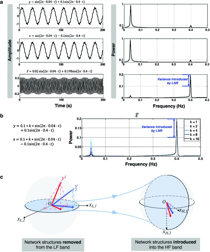
where / and correspond to the LF/HF components of and , respectively. is the estimated scaling coefficient for the model: . Since is dominated by LF components in observation/nuisance factors, subtracting from y_H may introduce rather than remove nuisance variance in the HF parts of data. A toy illustration of the issue is shown in Figure 1a, b.

FIG. 1.

Illustration of WB-LNR. (a) WB-LNR can introduce additional variance into the HF band of fMRI time series. Here, measurement y and nuisance regressor x both have low (0.04 Hz) and high (0.4 Hz)-frequency components. The cleaned signal ɛ [from Eqn. (3)] on the bottom includes a large HF contamination introduced by WB-LNR from the LF component. (b) Introduced variance as a function of the ratio k of LF and HF fluctuation amplitudes. (c) Illustration of how RSFC at low frequencies is twisted and passed to the HF band of fMRI data through WB-LNR. See text description in the Artificial network patterns introduced in HF bands section. fMRI, functional magnetic resonance imaging; HF, high-frequency; LF, low-frequency; LNR, linear nuisance regression; RSFC, resting-state functional connectivity; WB, whole-band. Color images available online at www.liebertpub.com/brain

Artificial network patterns introduced in HF bands

Apparently, the HF components of X_H will be introduced in every voxel with a scaling coefficient indicating the amount of LF variance explained by each specific nuisance source, that is, a globally correlated structure reflecting the contamination from each nuisance source will be added to y_H.

More importantly, it has recently been demonstrated by Bright and Murphy (2015) that the regressed noise () in the conventional LF band contains RS network structures, which can be discernable even if only two physiological regressors are employed. Being finite and stochastic samples of the nuisance factors and brain spontaneous activity, columns of X_L and functional information inherent in y_L cannot be perfectly orthogonal to each other despite that nuisance artifacts and brain signals are uncorrelated from the mathematical expectation perspective. This argument can be better conceptualized under the extreme condition where X_L is full rank and the number of nuisance regressors equals the number of time frames, in which case all the information (neural signals as well as noise) will be passed on to the removed variance, that is, . Therefore, the removed variance will inevitably contain part of the neural signals as well as true noisy fluctuations. Furthermore, as carries partial information inherent in , the introduced variance will thus inherit corrupted network information from the LF RS networks.

Figure 1c offers an intuitive view on how correlated structures in the LF bands are deformed and passed into HF bands through LNR. In the simplified case, brain functional information is described by a three-dimensional (3D) space (each voxel only contains three time frames), the time series is denoised with two nuisance regressors (x₁ and x₂), and the LNR process is dominated by LF fluctuations. For two correlated (not orthogonal to each other) time series y¹ and y² in the 3D space, their correlations are deformed through dimensionality reduction (projection onto the plane spanned by and ), changes of bases (distinct amplitudes and interdependence structures between / and /, rotation from the two-dimensional plane spanned by / to that spanned by / is highlighted by blue arrows), and then reintroduced into high frequencies through regression analysis.

Collectively, we have shown the concept that WB-LNR can introduce variance with globally correlated information as well as spurious network structures into the HF band of the observed data.

Materials and Methods

Data acquisition

Ten healthy subjects (4 females, aged 36 ± 12 years) recruited from the Stanford community participated in the current study. FMRI data were collected with a 3T scanner (GE Signa 750, Milwaukee, WI) with a 32-channel radio frequency coil (NOVA Medical, Wilmington, MA). A simultaneous multislice echo planar imaging (EPI) with blipped controlled aliasing in parallel imaging (CAIPI) sequence (Setsompop et al., 2012) was used for T2*-weighted functional imaging (TR/echo time [TE] = 350/30 msec, multiband acceleration factor = 6, CAIPI shift of field of view [FOV]/3, FOV = 220 cm, flip angle = 40°, 30 axial slices, voxel size 3.14 × 3.14 × 4 mm³). Each subject underwent a 10-min RS scan and an additional 7-sec scan with reversed phase encoding directions (to correct for susceptibility-induced distortions). Respiration and cardiac (pulse oximetry) data were recorded using the scanner's built-in physiological monitoring system.

Basic preprocessing

After reconstruction, data were corrected for susceptibility-induced distortions using the FSL TOPUP toolbox (http://fsl.fmrib.ox.ac.uk/fsl/fslwiki/TOPUP). The first 29 frames (∼10 sec) of each scan were discarded to allow the MR signal to achieve T1 equilibration. Basic preprocessing steps included time slice correction and removal of linear and quadratic scanner drifts with custom C and MATLAB routines. Physiological fluctuations synchronized with cardiac/respiratory cycles were removed using RETROICOR (Glover et al., 2000). Subjects' data were normalized to the Montreal Neurological Institute (MNI) template for the ensuing analysis (extrapolated to 2 × 2 × 2 mm³ resolution).

Construction of nuisance regressors

Combinations of nuisance regressors routinely employed in RS analyses were examined, as detailed in Table 1. The regressors were estimated from data post basic preprocessing in the Basic preprocessing section (real dataset).

Table 1.

Sets of Nuisance Regressors Examined in the Presented Work

Regressor	Description	No. of regressors
mot6	3 translational and 3 rotational motion estimates	6
mot12	mot6 + 6 temporal derivative terms	12
mot24	mot12 + 12 squared terms (Friston et al., 1996)	24
csf + white	Signals averaged within 3-mm radius spheres centered at MNI (26, −12, 35) for white matter and (19, −33, 18) for CSF	2
Gs	Signal averaged across voxels of the whole brain	1
mot6 + comb	mot6 + csf + white + 4 physiological regressors from RVHRcor (2 low-frequency fluctuating time series induced by cardiac/respiratory variations and their temporal derivative terms) (Chang et al., 2009)	12
mot24 + comb	mot24 + csf + white + 4 physiological regressors from RVHRcor	30
mot24 + comb + gs	mot6 + csf + white + 4 physiological regressors from RVHRcor + gs	31

CSF, cerebrospinal fluid; MNI, Montreal Neurological Institute.

Simulation

The simulations aimed at examining the concept that WB-LNR could yield spurious HF-RSFC, even if there exist no correlated structures at high frequencies in the raw dataset.

To this end, a dummy dataset having only LF fluctuations was created from the real dataset by eliminating any possible HF correlations. Specifically, we took the Fourier transform of each voxel's time series for each subject, scrambled the phases of components above 0.2 Hz, and then inversely Fourier transformed back to the temporal domain (i.e., the power distribution and temporal autocorrelation structure of each voxel's time series was unaltered). Consequently, RSFC of the created dummy dataset was identical with that of the real dataset at frequencies below 0.2 Hz, but contained no structured information above 0.2 Hz.

Next, regressors derived from the real dataset (see Construction of nuisance regressors section) were linearly projected out of the dummy dataset. The cleaned dummy dataset was further filtered into three different bands: LB (0–0.2 Hz), HB1 (0.4–1.4 Hz), and HB2 (0.8–1.4 Hz), within which FCs of two RS networks—the default mode network (DMN, the most active network at rest) and visual network (VN, a robust sensory network commonly observed at rest)—were estimated, respectively. The network patterns were generated by linearly correlating the time series of each brain voxel and a pivotal seed voxel in each network—MNI coordinate (0, −56, 26) (posterior cingulate cortex [PCC]) for DMN and (−32, −88, 2) (left occipital lobe) for VN.

In the simulation and ensuing real dataset analysis, we chose 0.2 Hz as the upper threshold for LF band signals because it resides closer to the spectrum elbows than the more commonly employed 0.1 Hz for most brain regions of interest (ROIs) based on the present dataset and power plots (Gohel and Biswal, 2015, Fig. 1). For HF signals, 0.4 Hz was selected as the lower bound threshold so that HB1/HB2 span frequencies not supported by the canonical HRF and are free from potential residual confounds induced by respiratory movement.

Analysis of real dataset

Similar to the simulation analysis, a cleaned real dataset was first generated by WB-LNR with regressors constructed as above (Construction of nuisance regressors section). We then quantified the variance removed (or introduced) by WB-LNR in different frequency bands (LB, HB1, HB2). The variances of signals averaged within brain functional ROIs were compared before and after WB-LNR. The ROIs were reported by Shirer and colleagues (2012) (http://findlab.stanford.edu/functional_ROIs.html) and only those containing >200 voxels were selected; each ROI mask was further eroded to contain 100 voxels, 2 × 2 × 2 mm³ cubical resolution.

Furthermore, the DMN/VN from real and cleaned real datasets were generated using identical seed-based approaches as those employed in the simulations and compared to evaluate the impacts of WB-LNR on the observed LF/HF network patterns.

RETROICOR was employed as a default preprocessing step and excluded from the LNR examination here because the spectra of modeled fluctuations peaked at the cardiac/respiratory frequencies (∼1/0.2 Hz), not falling into the category described in the Background: WB-LNR section. However, RETROICOR models the quasi-periodic noise induced by cardiac/respiratory cycles based on external physiological recordings and projects them out of the fMRI time series through linear regression as well. Due to the jittering of cardiac/respiratory cycles in practical conditions, the modeled fluctuations inevitably contain HF components and may thus interfere with HF components of the real signal. To eliminate such concerns that the observed HF-RSFC originated partly from RETROICOR, connectivity analyses were also conducted on the real dataset before RETROICOR and LNR.

An overview of the simulation and analysis is shown in Figure 2.

FIG. 2.

Overview of the simulation and analysis scheme. DMN, default mode network; VN, visual network.

Results

Power spectra of the regressors

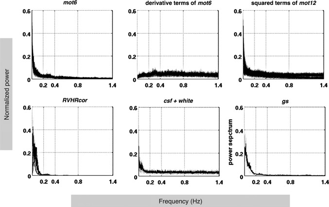
Figure 3 shows the frequency spectra of the estimated nuisance regressors (Table 1). Regressors (mot6 and its squared terms, csf + white, gs) are characterized by dominating LF fluctuations and HF components persisting up to 1.4 Hz (the upper limit of frequencies resolved by TR = 0.35 sec). Hence, every regressor set listed in Table 1 contains components that could potentially cause spurious HF-RSFC based on the Background: WB-LNR section. Besides, the derivative terms of six motion parameters spread flatly across the entire frequency band. Regressors from RVHRcor decay quickly to zero beyond 0.4 Hz because they are obtained by convolving the variability waveforms of heart rates and respiratory volumes with modeled response functions (fitted by LF gamma functions) (Chang et al., 2009).

FIG. 3.

Power spectra of nuisance regressors (see Table 1 for descriptions) constructed from real dataset (see Construction of nuisance regressors section). The time series of each regressor is normalized to z-score (demeaned and scaled to unit variance) before spectrum estimation for each subject. Subject means (black lines) and standard deviations (shaded gray area) of the z-score power spectra are plotted.

Dummy dataset: spurious HF network structures introduced by WB-LNR

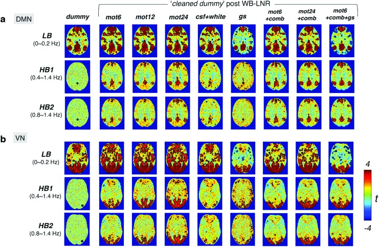
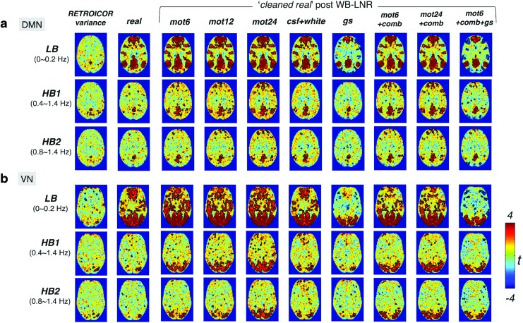
DMN/VN maps of the cleaned dummy dataset within three different frequency bands—LB (<0.2 Hz), HB1 (0.4–1.4 Hz), and HB2 (0.8–1.4 Hz)—are displayed in Figure 4. Robust networks are demonstrated in LB, with minor modifications depending on the regressors employed. No regions show significant correlations with the network seed before LNR (dummy column). By contrast, several brain regions commonly reported as part of the DMN/VN surpass the uncorrected threshold (p < 0.05) for both HB1 and HB2 post-LNR, even with as few as two nuisance regressors (csf + white). Briefly, the spurious HF functional connectivity introduced by LNR becomes more and more like that of the LF network structures (LB, dummy) as the number of regressors increases. The close resemblance of network patterns in HB1 and HB2 suggests that the contrast (introduced functional signals by LNR)-to-noise (unordered fluctuations in the dummy dataset) ratios do not differ significantly between 0.4–0.8 Hz and 0.8–1.4 Hz bands.

FIG. 4.

The group-level t-map of DMN(a)/VN(b) within different frequency bands post-WB-LNR (the cleaned dummy dataset, across 10 subjects). Regions inside the black contour surpass the statistical threshold (p < 0.05, uncorrected). Note false HF-RSFC introduced by LNR to varying degrees depending on regressors. Color images available online at www.liebertpub.com/brain

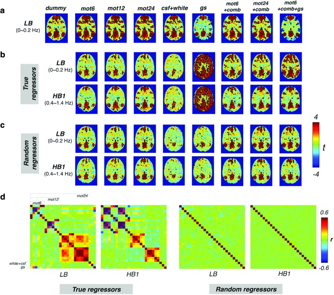
Figure 5a repeats the LB DMN results from Figure 4; (b) shows DMN connectivity maps generated from the noisy variance projected out of the LB, and introduced into HB1 of the dummy dataset. The relationship between the spurious HF-RSFC and the true LF-RSFC in the dataset is in accordance with the theory introduced in the Artificial network patterns introduced in HF bands section. Pattern alternations due to dimensionality differences, change of bases (interdependence structure of the regressors across different frequency bands), and exemplification of nuisance factors (globally correlated effect) can be explicitly observed in the results.

FIG. 5.

(a) The group-level t-map of DMN in the LB of the cleaned dummy dataset from Figure 4a for comparison with Figure 5b, c; (b) LB/HB1 of the removed variance using true regressors; and (c) LB/HB1 of the removed variance using random regressors. Correlation values at the subject level are Fisher z transformed before entering the group-level analysis except for True regressors, gs, which display the group t-value based on direct correlation values (r = ±1 for a single regressor). Regions inside the black contour surpass the statistical threshold (p < 0.05, uncorrected). (d) Linear correlation matrices of true/random nuisance regressors within different frequency bands. Color images available online at www.liebertpub.com/brain

Since the number of employed nuisance regressors (≤31) is  than the number of collected temporal frames (1681), the removed variance in the conventional band (Fig. 5b, LB, true regressors) only contains part of the LF connectivity information. Thus, in line with the results in Figure 4, the projected DMN more closely resembles the raw connectivity patterns (Fig. 5a, LB, dummy) as the number of regressors increases.

The interdependence structure of nuisance regressors at high frequencies differs from that at low frequencies (Fig. 5d, true regressors). As discussed earlier, the structured variance introduced into high frequencies by LNR deviates from that projected out of the LF fluctuations in spite of the identical scaling coefficient . This is more evidently revealed in comparison with the case dummy dataset regressing against a set of random regressors (generated by randomly shuffling the WB phases of each true regressor, with the process repeated until the linear correlation between the generated regressor and true regressor is below 0.1). These random regressors share identical frequency distributions as the true regressors, but are not related to any nuisance metrics (e.g., motion noise) in the real dataset. As regressors generated thereby possess similarly independent structures across frequencies (Fig. 5d, random regressors), the projected networks in LB and introduced networks in HB1 are more alike (Fig. 5c).

Apart from neural activity-related information, the introduced HF-RSFC also maps the global impacts of each nuisance factor since the fitted parameter scales proportionally with the extent to which a voxel is contaminated by each specific nuisance source. For instance, in the variance regressed by one single global signal, most gray matter regions (with major contributions to the averaged signal) are positively correlated with the PCC seed using true regressors, whereas only key nodes of the DMN show up using random regressors (Fig. 5b, c, true regressors vs. random regressors, gs).

Real dataset: variance removed/introduced by LNR

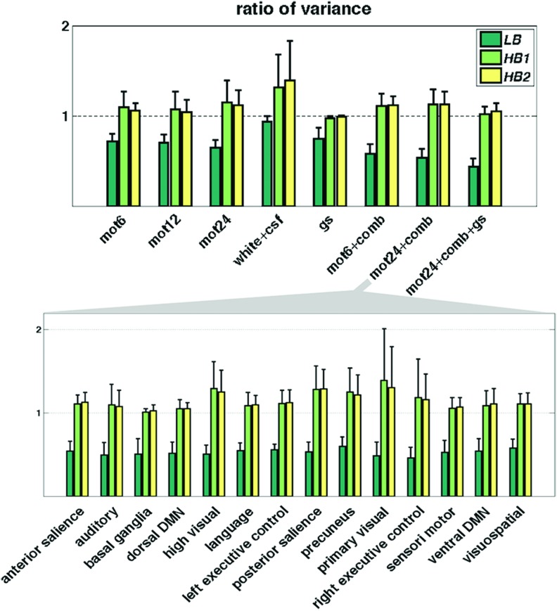
Figure 6 shows the ratio of signal variance postnuisance regression and before nuisance regression, averaged across different functional ROIs. As expected, variance is effectively reduced in LB, but increased in both HB1 and HB2 (consistently across different regressors and networks), corroborating that WB-LNR does bring in additional variance to the dataset.

FIG. 6.

The ratio of signal variance before and after WB-LNR (top, averaged across all the brain functional ROIs when tested against 0 using one-sample t-test, all passing the significance level p < 0.0001, Bonferroni corrected); an example of variance changes in different brain networks, postregression using mot24 + comb (bottom, averaged across ROIs within different RS networks). ROIs, regions of interest; RS, resting state. Color images available online at www.liebertpub.com/brain

Variances are modestly reduced if only the global signal is included in LNR, which may be explained by the facts that (1) the power contrast between HB1/HB2 and LB is more pronounced for global signal compared with other regressors (Fig. 3) and (2) cortical regions do share common HF fluctuations (either neural related or noisy) that are preserved through global averaging. Moreover, the introduced HF variance by mot24 + comb is reduced in conjunction with global signal (mot24 + comb + gs). This is possibly attributable to the fact that the global signal fits the LB fluctuations better than other modeled nuisance factors since it derives from massive averaging of the dataset itself and contains unwanted noise as well as neural activity underlying wide cortex regions. As a consequence, the global signal plays a pivotal role in the least-square fitting of LNR, downweighting the contribution from other regressors as well as the additional variance introduced to high frequencies.

Real dataset: spurious HF structures introduced by WB-LNR

DMN and VN connectivity maps of the real dataset are shown in Figure 7a, b, respectively. Correlated patterns in the variance removed by RETROICOR are minor for both networks (RETROICOR variance), eliminating the possibility that the observed HF-RSFC stems largely from regression procedures employed in the Basic preprocessing section. Pronounced DMN/VN are observed post-LNR, and the exhibited patterns are generally in line with the simulation results above.

FIG. 7.

The group-level (10 subjects) t-map of network patterns [(a) DMN, (b) VN] within different frequency bands post-WB-LNR (the cleaned real dataset). Regions inside the black contour surpass the statistical threshold (p < 0.05, uncorrected). Consistent with simulations, HF-RSFC is introduced by LNR to varying degrees depending on regressors. No prominent connectivity patterns are observed in the variance removed by RETROICOR (RETROICOR variance), suggesting that HF-RSFC observed in the real data HF-RSFC stems largely from WB-LNR instead of RETROICOR. Color images available online at www.liebertpub.com/brain

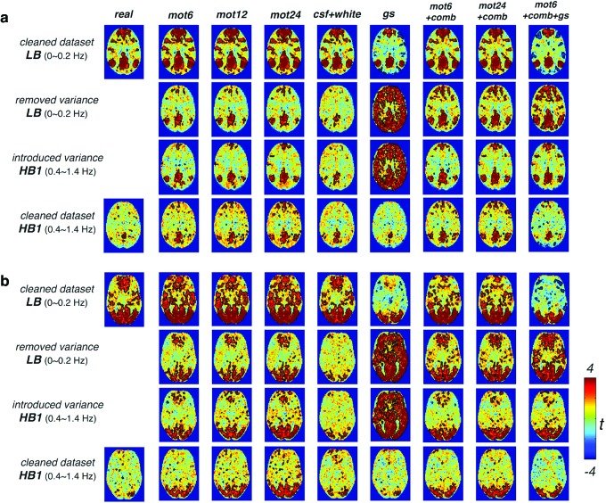
Contrasting the network patterns appeared in the cleaned real dataset (Fig. 8, cleaned dataset) and those inherent in the introduced variance (Fig. 8, introduced variance), the remarkable resemblance implies that the observed HF-RSFC is to a large extent artificially introduced by WB-LNR. Notably, despite that mot24 + comb + gs introduces minimal structured variance to the data (see variance plot in Fig. 6), that is, the effect size is tiny at the subject level, RSFC of the chosen two networks is already discernable at the group level for the relatively small subject size of 10.

FIG. 8.

Close resemblance between the group-level t-map of network patterns [(a) DMN, (b) VN] in the removed variance and cleaned real dataset post-LNR. Correlation values at the subject level are Fisher z transformed before entering the group-level analysis except for removed/introduced variance, gs, which display the group t value based on direct correlation values (r = ±1 for a single regressor). Color images available online at www.liebertpub.com/brain

Discussion and Conclusion

Simulations and real data analysis in the present study have demonstrated that WB-LNR can introduce additional variance with structured network patterns at frequencies not easily supported by BOLD mechanisms, which are discernable with as few as two nuisance regressors (csf + white), and become more and more prominent as the number of regressors increases. Although stemming from spontaneous activity in the conventional band, this artificially introduced HF-RSFC is not identical with LF-RSFC due to frequency-variant interdependence structures of nuisance regressors. Moreover, since the regressors are associated with various noisy confounds (e.g., motion), the artifactual network patterns at higher frequencies naturally amplify the influence of non-neurally related artifacts compared with true functional connectivity at lower frequencies.

Similar concerns extending to regressors identified by data-driven approaches

So far, we have discussed the case where nuisance fluctuations are identified from fixed models as specified in Table 1. Alternatively, nuisance fluctuations can also be identified through data-driven decompositions, for example, principal component analysis (PCA) and independent component analysis (ICA). Such approaches first decompose the raw data into orthogonal or independent components and exert certain criteria to eliminate uninteresting components by linearly regressing the associated time series out of the raw data (e.g., Griffanti et al., 2014; Kundu et al., 2012, 2013; Olafsson et al., 2015; Salimi-Khorshidi et al., 2014; Thomas et al., 2002). If the temporal space spanned by the uninteresting non-neural components contains more power in LF than HF fluctuations (since it is likely linked with or consists largely of common LF-driven nuisance factors [e.g., motion, physiological noise, shown in Fig. 3]), similar concerns of introducing spurious HF RSFC can still exist.

Notably, apart from the regression procedure, HF structures of the data can also be contaminated by dimensionality reduction using low-rank temporal PCA if not prewhitened with respect to voxel-wise temporal noise covariance. Likewise, similar concerns can extend to temporal ICA, which commonly employs PCA or singular vector decomposition as a prior dimensionality reduction step. See Supplementary Data A (Supplementary Data are available online at www.liebertpub.com/brain) for detailed discussion.

Revisit of the existing findings on HF connectivity

While two HF bands (0.4–1.4 Hz and 0.8–1.4 Hz) were investigated in the present study, LF-RSFC can be extended into any HF bands through the fitted scaling parameters as long as the nuisance regressors contain tiny (negligible compared with LF bands), but nonzero, fluctuations at the examined frequencies. Whereas most regressors are extracted from the raw data or external psychometric measurement devices, where various broad band noise sources exist, the criteria can be easily satisfied. Because these HF fluctuations introduced by WB-LNR reflect both the distorted transformation of LF-RSFC and the globally correlated structure indicating voxel-wise contamination from each specific nuisance factor, one would expect disparate network characteristics in HF/LF bands at both the subject and group levels (frequency behavior of certain nuisance factors, e.g., physiological noise, is not likely to differ substantially across subjects).

We have previously examined the TE dependence of correlated RSFC amplitudes and demonstrated coexistence of both BOLD-like and non-BOLD-like contributions up to 0.5 Hz (Chen and Glover, 2015). In the original analysis, WB-LNR with regressor set (mot6 + comb) was used, falling within the caveats discussed here. Since the structured noise introduced to HF bands derives from both RSFC (BOLD mechanism) and noisy fluctuations induced by nuisance sources (non-BOLD mechanism) at lower frequencies, it naturally contains both BOLD-like and non-BOLD-like variance. We therefore reestimated the TE dependence of signal amplitudes with matched-band LNR strategy (filtering both signals and regressors into different frequency bands so that LF and HF signals would not interfere with each other, then performing LNR within each band). The results are shown in Supplementary Figure S1. The value of the fitted slope (TE-dependent BOLD component) increases modestly within 0.01–0.1 Hz, which can be explained by a slight decrease of the mean correlated signal amplitude across TEs (in the normalization procedure, see captions of Supplementary Fig. S1) post matched-band LNR compared with WB-LNR. Notably, values of fitted slopes drop instead of increasing explicitly compared with WB-LNR >0.1 Hz, particularly the linear TE dependence of frequency band (0.4–0.5 Hz) is no longer significant at the confidence level (). Such results suggest that our previous observations indeed stemmed partly from BOLD-like fluctuations introduced by WB-LNR and only support BOLD-like components up to 0.4 Hz. In contrast, extrapolates of fitted signal amplitudes (non-BOLD-like components) change very slightly at TE = 0 msec across different frequencies. This is possibly because fluctuations induced by nuisance factors are very minor in the DMN of examined subjects or the associated non-BOLD-like components are negligible compared with other non-BOLD-like sources in the DMN.

Collectively, HF-RSFC artificially introduced by WB-LNR is unbounded, frequency dependent, and originates from both BOLD/non-BOLD mechanisms, mirroring those major characteristics of HF spontaneous activity reported so far. Thus, there exists the possibility that the HF-RSFCs observed in previous literature, particularly those well beyond the band permitted by the canonical HRF model, are partly induced by improper preprocessing (e.g., WB-LNR or various PCA/ICA denoising approaches). Due to variations in acquisition protocols, subjects, and versatile preprocessing operations, conclusions based on our results may not generalize to earlier studies. However, it is advised and worthwhile to reexamine the published conclusions with careful attention to preprocessing to exclude the potential confounds proposed here, as in the way we reanalyzed the previous study.

Implications for preprocessing of RS analysis

Hallquist and colleagues (2013) have demonstrated that spectral mismatch in nuisance regression (signals are bandpass filtered, while the regressors are unfiltered) would reintroduce nuisance-related variations from the suppressed band to the filtered signals and further advocated to perform bandpass filtering of both signals and regressors simultaneously (matched-band filtering). However, such matched-band filtering approach may only be valid under scenarios where the scaling factor is relatively constant across examined frequencies or the frequency of interest dominates the pass band. We therefore advise future studies (interested in frequency-specific behaviors of RSFC in a relatively broad band) to check the variability of across the resolved frequencies (e.g., by filtering both signals and regressors into narrower sub-bands and performing matched-band LNR) before determining the denoising strategy. Briefly, if varies within the entire band, simultaneously filtering of both signals and regressors into specific bands before LNR is preferred; if is relatively stable across the examined frequencies, regression before filtering may result in more reliable due to increased effective degrees of freedom and statistical power. However, caution should be exercised that bandpass filtering can spread motion artifacts in time (Carp, 2013).

Apart from exploiting frequency-dependent behavior of spontaneous activity, there has been growing interest in collecting RS data using accelerated acquisitions with the expectation of increased statistical power (more sampling points within a fixed scan duration) and identification of cardiac/respiratory peaks in signal spectra (Boyacioglu et al., 2015; Feinberg et al., 2010; Griffanti et al., 2014; Posse et al., 2012). These investigations generally integrate across the entire frequency band resolved by the short TR without being interested in any particular frequency band. However, if frequencies beyond the conventional band contain less prominent network structures or have much lower CNR compared with the low-frequency activities (preliminary reanalyses of the real dataset without LNR result in very weak DMN and VN beyond 0.2 Hz, shown in Fig. 9), including HF signals in network analysis may possibly obscure instead of enhancing the existing connectivity patterns. Moreover, HF signals may have already been contaminated due to preprocessing operations driven by LF fluctuations. Thus, RSFC analysis may benefit from moderate low-pass filtering. For instance, Olafsson and colleagues (2015) reported that low-pass filtering resulted in a significantly greater or comparable number of BOLD-like components as the WB data in different subjects.

FIG. 9.

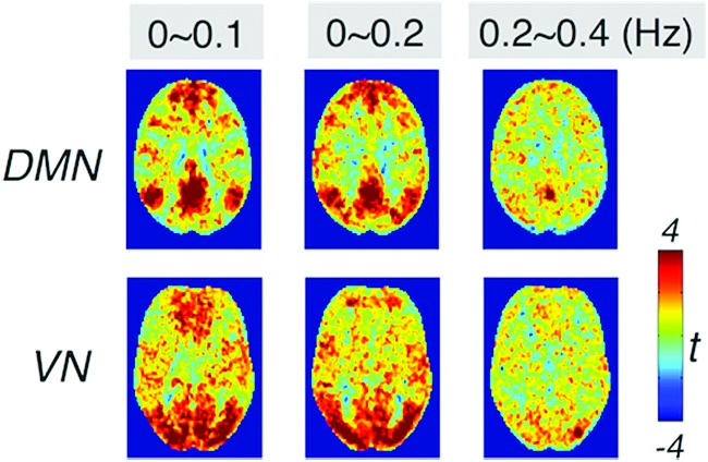
The group-level (10 subjects) t-map of DMN and VN patterns of the real dataset (without LNR) in different frequency bands. Color images available online at www.liebertpub.com/brain

Acknowledgments

Funding of this study is supported by NIH P41EB15891, R01 NS066506, R01 NS047607, R01 DK092241, and GE healthcare. The authors also gratefully acknowledge two anonymous reviewers, whose constructive comments have greatly improved the quality of this article.

Author Disclosure Statement

No competing financial interests exist.

References

- Boubela RN, Kalcher K, Huf W, Kronnerwetter C, Filzmoser P, Moser E, 2013. Beyond noise: using temporal ICA to extract meaningful information from high-frequency fMRI signal fluctuations during rest. Front Hum Neurosci 7:168. [DOI] [PMC free article] [PubMed] [Google Scholar]
- Boyacioglu R, Beckmann CF, Barth M. 2013. An investigation of RSN frequency spectra using ultra-fast generalized inverse imaging. Front Hum Neurosci 7:156. [DOI] [PMC free article] [PubMed] [Google Scholar]
- Boyacioglu R, Schulz J, Koopmans PJ, Barth M, Norris DG. 2015. Improved sensitivity and specificity for resting state and task fMRI with multiband multi-echo EPI compared to multi-echo EPI at 7 T. Neuroimage 119:352–361 [DOI] [PubMed] [Google Scholar]
- Bright MG, Murphy K. 2015. Is fMRI “noise” really noise? Resting state nuisance regressors remove variance with network structure. Neuroimage 114:158–169 [DOI] [PMC free article] [PubMed] [Google Scholar]
- Carp J. 2013. Optimizing the order of operations for movement scrubbing: comment on Power et al. Neuroimage 76:436–438 [DOI] [PubMed] [Google Scholar]
- Chang C, Cunningham JP, Glover GH. 2009. Influence of heart rate on the BOLD signal: the cardiac response function. Neuroimage 44:857–869 [DOI] [PMC free article] [PubMed] [Google Scholar]
- Chen JYE, Glover GH. 2015. BOLD fractional contribution to resting-state functional connectivity above 0.1 Hz. Neuroimage 107:207–218 [DOI] [PMC free article] [PubMed] [Google Scholar]
- Feinberg DA, Moeller S, Smith SM, Auerbach E, Ramanna S, Glasser MF, et al. . 2010. Multiplexed echo planar imaging for sub-second whole brain fMRI and fast diffusion imaging. PLoS One 5:e15710. [DOI] [PMC free article] [PubMed] [Google Scholar]
- Figley CR, Leitch JK, Stroman PW. 2010. In contrast to BOLD: signal enhancement by extravascular water protons as an alternative mechanism of endogenous fMRI signal change. Magn Reson Imag 28:1234–1243 [DOI] [PubMed] [Google Scholar]
- Friston KJ, Williams S, Howard R, Frackowiak RS, Turner R. 1996. Movement-related effects in fMRI time-series. Magn Reson Med 35:346–355 [DOI] [PubMed] [Google Scholar]
- Gao JH, Liu HL. 2012. Inflow effects on functional MRI. Neuroimage 62:1035–1039 [DOI] [PubMed] [Google Scholar]
- Glover GH, Li TQ, Ress D. 2000. Image-based method for retrospective correction of physiological motion effects in fMRI: RETROICOR. Magn Reson Med 44:162–167 [DOI] [PubMed] [Google Scholar]
- Gohel SR, Biswal BB. 2015. Functional integration between brain regions at rest occurs in multiple-frequency bands. Brain Connect 5:23–34 [DOI] [PMC free article] [PubMed] [Google Scholar]
- Griffanti L, Salimi-Khorshidi G, Beckmann CF, Auerbach EJ, Douaud G, Sexton CE, et al. . 2014. ICA-based artefact removal and accelerated fMRI acquisition for improved resting state network imaging. Neuroimage 95:232–247 [DOI] [PMC free article] [PubMed] [Google Scholar]
- Hallquist MN, Hwang K, Luna B. 2013. The nuisance of nuisance regression: spectral misspecification in a common approach to resting-state fMRI preprocessing reintroduces noise and obscures functional connectivity. Neuroimage 82:208–225 [DOI] [PMC free article] [PubMed] [Google Scholar]
- Kundu P, Brenowitz ND, Voon V, Worbe Y, Vertes PE, Inati SJ, et al. . 2013. Integrated strategy for improving functional connectivity mapping using multiecho fMRI. Proc Natl Acad Sci U S A 110:16187–16192 [DOI] [PMC free article] [PubMed] [Google Scholar]
- Kundu P, Inati SJ, Evans JW, Luh WM, Bandettini PA. 2012. Differentiating BOLD and non-BOLD signals in fMRI time series using multi-echo EPI. Neuroimage 60:1759–1770 [DOI] [PMC free article] [PubMed] [Google Scholar]
- Le Bihan D. 2003. Looking into the functional architecture of the brain with diffusion MRI. Nat Rev Neurosci 4:469–480 [DOI] [PubMed] [Google Scholar]
- Lee HL, Zahneisen B, Hugger T, Levan P, Hennig J. 2013. Tracking dynamic resting-state networks at higher frequencies using MR-encephalography. Neuroimage 65:216–222 [DOI] [PubMed] [Google Scholar]
- Lin FH, Chu YH, Hsu YC, Lin JFL, Tsai KWK, Tsai SY, Kuo WJ. 2015. Significant feed-forward connectivity revealed by high frequency components of BOLD fMRI signals. Neuroimage 121:69–77 [DOI] [PubMed] [Google Scholar]
- Morgan VL, Rogers BP, Abou-Khalil B. 2015. Segmentation of the thalamus based on BOLD frequencies affected in temporal lobe epilepsy. Epilepsia 56:1819–1827 [DOI] [PMC free article] [PubMed] [Google Scholar]
- Niazy RK, Xie JY, Miller K, Beckmann CF, Smith SM. 2011. Spectral characteristics of resting state networks. Prog Brain Res 193:259–276 [DOI] [PubMed] [Google Scholar]
- Olafsson V, Kundu P, Wong EC, Bandettini PA, Liu TT. 2015. Enhanced identification of BOLD-like components with multi-echo simultaneous multi-slice (MESMS) fMRI and multi-echo ICA. Neuroimage 112:43–51 [DOI] [PMC free article] [PubMed] [Google Scholar]
- Posse S, Ackley E, Mutihac R, Rick J, Shane M, Murray-Krezan C, et al. . 2012. Enhancement of temporal resolution and BOLD sensitivity in real-time fMRI using multi-slab echo-volumar imaging. Neuroimage 61:115–130 [DOI] [PMC free article] [PubMed] [Google Scholar]
- Power JD, Mitra A, Laumann TO, Snyder AZ, Schlaggar BL, Petersen SE. 2014. Methods to detect, characterize, and remove motion artifact in resting state fMRI. Neuroimage 84:320–341 [DOI] [PMC free article] [PubMed] [Google Scholar]
- Salimi-Khorshidi G, Douaud G, Beckmann CF, Glasser MF, Griffanti L, Smith SM. 2014. Automatic denoising of functional MRI data: combining independent component analysis and hierarchical fusion of classifiers. Neuroimage 90:449–468 [DOI] [PMC free article] [PubMed] [Google Scholar]
- Satterthwaite TD, Elliott MA, Gerraty RT, Ruparel K, Loughead J, Calkins ME, et al. . 2013. An improved framework for confound regression and filtering for control of motion artifact in the preprocessing of resting-state functional connectivity data. Neuroimage 64:240–256 [DOI] [PMC free article] [PubMed] [Google Scholar]
- Setsompop K, Gagoski BA, Polimeni JR, Witzel T, Wedeen VJ, Wald LL. 2012. Blipped-controlled aliasing in parallel imaging for simultaneous multislice echo planar imaging with reduced g-factor penalty. Magn Reson Med 67:1210–1224 [DOI] [PMC free article] [PubMed] [Google Scholar]
- Shirer WR, Ryali S, Rykhlevskaia E, Menon V, Greicius MD. 2012. Decoding subject-driven cognitive states with whole-brain connectivity patterns. Cereb Cortex 22:158–165 [DOI] [PMC free article] [PubMed] [Google Scholar]
- Smith-Collins APR, Luyt K, Heep A, Kauppinen RA. 2015. High frequency functional brain networks in neonates revealed by rapid acquisition resting state fMRI. Hum Brain Mapp 36:2483–2494 [DOI] [PMC free article] [PubMed] [Google Scholar]
- Sours C, Chen H, Roys S, Zhuo J, Varshney A, Gullapalli RP. 2015. Investigation of multiple frequency ranges using discrete wavelet decomposition of resting-state functional connectivity in mild traumatic brain injury patients. Brain Connect 5:442–450 [DOI] [PMC free article] [PubMed] [Google Scholar]
- Thomas CG, Harshman RA, Menon RS. 2002. Noise reduction in BOLD-based fMRI using component analysis. Neuroimage 17:1521–1537 [DOI] [PubMed] [Google Scholar]
- Van Dijk KRA, Sabuncu MR, Buckner RL. 2012. The influence of head motion on intrinsic functional connectivity MRI. Neuroimage 59:431–438 [DOI] [PMC free article] [PubMed] [Google Scholar]
- Wang J, Zhang Z, Ji GJ, Xu Q, Huang Y, Wang Z, et al. . 2015. Frequency-specific alterations of local synchronization in idiopathic generalized epilepsy. Medicine (Baltimore) 94:e1374. [DOI] [PMC free article] [PubMed] [Google Scholar]
- Wu CWW, Gu H, Lu HB, Stein EA, Chen JH, Yang YH. 2008. Frequency specificity of functional connectivity in brain networks. Neuroimage 42:1047–1055 [DOI] [PMC free article] [PubMed] [Google Scholar]
- Yuan BK, Wang J, Zang YF, Liu DQ. 2014. Amplitude differences in high-frequency fMRI signals between eyes open and eyes closed resting states. Front Hum Neurosci 8:503. [DOI] [PMC free article] [PubMed] [Google Scholar]
Associated Data
This section collects any data citations, data availability statements, or supplementary materials included in this article.