A single weighting approach to analyze respondent-driven sampling data

Abstract

Background and objectives:

Respondent-driven sampling (RDS) is widely used to sample hidden populations and RDS data are analyzed using specially designed RDS analysis tool (RDSAT). RDSAT estimates parameters such as proportions. Analysis with RDSAT requires separate weight assignment for individual variables even in a single individual; hence, regression analysis is a problem. RDS-analyst is another advanced software that can perform three methods of estimates, namely, successive sampling method, RDS I and RDS II. All of these are in the process of refinement and need special skill to perform analysis. We propose a simple approach to analyze RDS data for comprehensive statistical analysis using any standard statistical software.

Methods:

We proposed an approach (RDS-MOD - respondent driven sampling-modified) that determines a single normalized weight (similar to RDS II of Volz-Heckathorn) for each participant. This approach converts the RDS data into clustered data to account the pre-existing relationship between recruits and the recruiters. Further, Taylor's linearization method was proposed for calculating confidence intervals for the estimates. Generalized estimating equation approach was used for regression analysis and parameter estimates of different software were compared.

Results:

The parameter estimates such as proportions obtained by our approach were matched with those from currently available special software for RDS data.

Interpretation & conclusions:

The proposed weight was comparable to different weights generated by RDSAT. The estimates were comparable to that by RDS II approach. RDS-MOD provided an efficient and easy-to-use method of estimation and regression accounting inter-individual recruits’ dependence.

It is difficult to map and develop sampling frames for hard-to-reach and hidden populations such as injecting drug users (IDUs) or men having sex with men (MSM) due to privacy concerns and closed knit nature of the groups. Hence, conventional probability-based sampling methods cannot be applied to sample them. Snowball sampling, key informants sampling and targeted sampling are some of the previously described sampling methods for this population1,2,3. However, all these methods have their own limitations and known biases4. Slightly modified form of snowball method has been used to count the rare events such as maternal mortality5.

Respondent-driven sampling (RDS) was introduced by Heckathorn to sample hidden and hard-to-reach populations. RDS is a modified form of snowball sampling, with a system for assigning weights to compensate for the unequal selection probability4. RDS starts with identifying prototype individuals known to represent a specific hidden or hard-to-reach population termed as ‘seeds’. In turn, seeds recruit the first wave of respondents and then the first-wave respondents recruit the second wave of respondents and such successive ‘waves’ help recruiting respondents until the desired sample size is reached. Although respondents recruit those with whom they have a pre-existing relationship, the primary expectation is that the respondents recruit randomly from their personal network6. The probability of inclusion is derived from the extension of Markov Chain (MC) theory and random walk on the network connecting the target population7,8,9,10. This theoretical framework forms the basis for calculating unbiased estimates. As the selection of seeds is non-random, the RDS data lack external validity11. However, with attainment of more than six waves, the sample composition is expected to stabilize and become independent of seeds4,12.

The existing software to analyze RDS data is RDS analysis tool (RDSAT), and it can generate only estimators13. Currently, RDSAT is in the stage of refinement and evolution. RDSAT uses bootstrapping to obtain confidence intervals (CIs) for estimates8,14. Goel and Salganik introduced an MC argument for population mixing10. They proposed an estimator by weighting the variable obtained from the size of the participants’ network and the network pattern focusing on relationships within the network. However, individualized weights have to be obtained for each variable and incorporated in the estimation procedure. Therefore, only one estimate can be made at a time and hence it consumes more time for data analysis. In addition, regression analysis is not possible with RDSAT. Efforts were made to adopt RDS data to regression analysis for adjusting estimates to reflect the targeted population12,15. Exporting of individualized weights of a chosen variable from RDSAT for conducting univariate regression analysis was attempted. Also, multivariate-weighted regression using the weights generated by RDSAT was attempted16. However, RDSAT produces as many weights as the number of variables for each participant and this is the problem in applying multivariate regression to RDS data.

Volz and Heckathorn6 generalized Horvitz-Thompson estimator to adopt RDS estimation to survey sampling (RDS II) and this was found to outperform the MC method. This was a single weight per participant approach unlike RDSAT's multiple weights per participant. Their approach made it possible to do regression analysis of RDS data. Calculation of variance analytically was made possible, but the problem of calculating CIs for a smaller group of respondents remained unresolved. Other approaches that have been proposed for analysis of RDS data are RDS-MR estimate (for analyzing continuous variables controlling for differential recruitment), RDS-SS estimates (for eliminating the condition of selection with replacement) and variance estimation6,17,18,19. All are currently in various stages of development20. RDS analyst (RDS-A) is the currently available most advanced software, but the problem with small samples and calculation of CIs for the estimation of cross-classified data remain a problem21 and it adopts bootstrap approach for the calculation of CIs. Thus, we need an approach or interface that allows use of RDS data in standard statistical applications and software.

The objective was to propose and validate a new two-step approach termed as RDS-MOD for analyzing RDS data. We hypothesized that determining a single normalized weight for each participant (irrespective of number of variables) and transforming RDS data into clustered data without affecting the recruitment pattern (sequence and equilibrium) would enable calculating CIs of the estimates including regression coefficients analytically in case of RDS data.

Material & Methods

The RDS-MOD was applied to a real dataset from India as well as four datasets available in public domain to estimate various parameters and their CIs. In addition, three real datasets were obtained and estimates were presented. STATA SVY module was used for analysis. Taylor method of linearization was applied to calculate standard errors (SEs) of estimates22. The precision of the proposed estimates was assessed based on the length of the CIs.

Data sources

Indian dataset: We used the first round data of Integrated Behavioural and Biological Assessment (IBBA) conducted in Churachandpur District of Manipur State, India, during the first quarter of 2006 on 419 IDUs recruited using RDS23,24. Three more datasets of the same survey were also obtained and HIV prevalence estimates were presented.

The datasets available in public domain were: (i) 1-3: Three simulated datasets of ‘RDS-A’ module. The datasets were faux (RDS); fauxsycamore (RDS) and fauxmadrona (RDS)21. (ii) 4: Jazz musicians dataset of RDSAT 7.1.4625.

Statistical analysis: Bland–Altman method was used to compare the single weight generated by RDS-MOD and the individualized weights generated by RDSAT for different variables of Churachandpur data26. The parameters and their 95 per cent CIs were estimated. The CIs were obtained as an output of SVY module of STATA using linearization and replication method for the calculation of SEs27. For multiple regression analysis, weighted generalized estimation equation (WGEE) was used.

For analysis, RDSAT 6.0.1(Cornell University Ithaca, NY), RDS-A, STATA 10 (Stata Corp, Texas USA); and SAS (Enterprise edition 4.3, SAS Institute, Cary, North Carolina, USA) were used. Drawing of network was performed by NetDraw 2.090. (Borgatti S.P, NetDraw Software for Network Visualization, Lexington, NY).

Data analysis by new approach (RDS-MOD)

Derivation of single weight and estimation method: Under the assumption in this chain referral sampling, the selection of a subject by a recruiter from his network is independent and is probability proportional to his degree (the number of men he knows and they know him) (d_i)8. A unique sampling weight Wi was derived for i^th participant. With these new weights and survey sampling module (SVY) of STATA, population parameters estimates were calculated27.

Formation of clusters

Formation of clusters in Churachandpur dataset (real dataset): The recruitment pattern is depicted as recruitment network diagram using ‘NetDraw’ in Fig. 1A. RDS data were converted into clusters by discarding all the seeds from network chains (Fig. 1B). All participants of the branch in a network chain after discarding a seed were considered as members of that cluster. An assumption was made that the clusters thus formed were independent though some traits (characteristic affiliation) of respective seeds would prevail upon the members of the clusters thus formed. However, this correlation would minimize or vanish with expanding waves and widening of gap between recruiters and recruits, thus diluting the trait of the seed. Further, the recruits within the clusters would have intra-cluster correlations that need to be addressed in any type of analysis. Had the number of seeds been more and independent, all recruits under a seed might have to be considered as independent clusters. In addition, with more number of clusters, the estimates could be better.

Fig. 1.

(A) RDS Network recruitment diagram of injecting drug users (IDUs) in Churachandpur district of Manipur State of India, 2006. (B) Network recruitment diagram of clusters created from the IDUs in Churachandpur district of Manipur State of India, 2006. All red circles: HIV +ve; All green triangles: HIV –ve. C1 to C17 are clusters formed from networks. Seeds are in larger size. Arrow-marks represent direction of recruitment chain. (NetDraw 2.090 software, Data Source: IBBA Round 1).

Formation of clusters in other example datasets: To perform RDS-MOD on other datasets (datasets in public domain) all the recruits under a seed were considered as cluster. Hence, the clusters would be independent if the seeds were independent. Thus, if there were ten seeds, ten clusters would be formed. For example, in fauxsycamore dataset of RDS-A, there were ten seeds. Therefore, ten clusters were formed for this analysis. For the dataset ‘faux (RDS)’, there was only one seed, and therefore, all the recruits were assumed to be from a single cluster. This was done to study the performance of RDS-MOD in situ ations where all the recruits under only one seed constituted a cluster.

Formation of clusters in yet other datasets (real datasets, viz. Bishnupur, Phek and Wokha): In Bishnupur dataset all seeds (nine) were removed. In the process, one cluster with single respondent was not considered. Thus, there were ten exclusions (nine seeds and one first-wave respondent).

In Phek and Wokha datasets, all recruits under a seed were considered as a cluster (nine clusters each).

Data analysis by RDSAT: The analysis tool RDSAT (6.0.1) was set to use average network size by adjusted mean values method. The number of re-samplings to determine bootstrap 95 per cent CI was set to 2500. The enhanced smoothing algorithm type was employed. Homophily (Hx) for each variable was obtained to understand the magnitude of the characteristic affiliation of recruiters with their recruits. The number of waves required for attaining equilibrium was also estimated by choosing a convergence radius of 0.02. We assumed a median base population as 10,000 and set 500 as bootstrap replication to analyze additional three real datasets (viz. Bishnupur, Phekh and Wokha).

Comparison of weights by RDS-MOD and the individualized weights of RDSAT for different variables under analysis: Single weight per study participant derived for RDS-MOD and the individualized weights generated by RDSAT for different variables were compared by Bland–Altman method26. The difference in weights by RDSAT and the calculated weight for RDS-MOD were plotted against the mean of the weights by these two approaches for a variable (Fig. 2). If the points on the Bland–Altman plot were uniformly scattered between the limits of agreement, it would suggest good agreement between the two weights by two different approaches. This analysis was performed to compare the individualized weights generated for each of variables by RDSAT and the single weight for each individual by RDS-MOD.

Fig. 2.

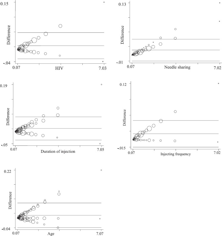
Agreement between the weights generated by RDSAT and RDS-MOD by Bland - Altman method. Source: Paul Seed, 2014. “BAPLOT: Stata module to produce Bland-Altman plots,” Statistical Software Components S457853, Boston College Department of Economics.

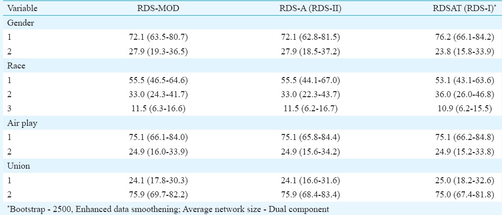
Comparison of estimates of RDS-MOD and RDS-A on example datasets: As our weights were similar to RDS II of Volz and Heckathorn6, RDS-MOD comparison of parameters by RDS-A (RDS II) would yield similar estimates but not the CIs. The comparison of estimates by different approaches using Churachandpur data is presented in Tables I and II. The results of comparison using the datasets, viz. faux, fauxmadrona, fauxsycamore of RDS-A and Jazz musicians’ dataset of RDSAT 7.1.46 are presented in Tables III and IV. In addition, HIV prevalence estimates were calculated both by RDS-A and RDS-MOD of yet another three real datasets (data not shown).

Table I.

Estimates of proportions of population parameters by respondent-driven sampling (RDS)-MOD (modified), RDS-A (analyst) and respondent-driven sampling analysis tool (RDSAT)- Churachandpur data

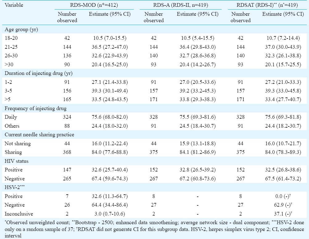
Table II.

Estimates of proportions of HIV status cross-classified by factors using respondent-driven sampling (RDS)-MOD (modified), RDS-A (analyst) and respondent-driven sampling analysis tool (RDSAT)- Churachandpur data

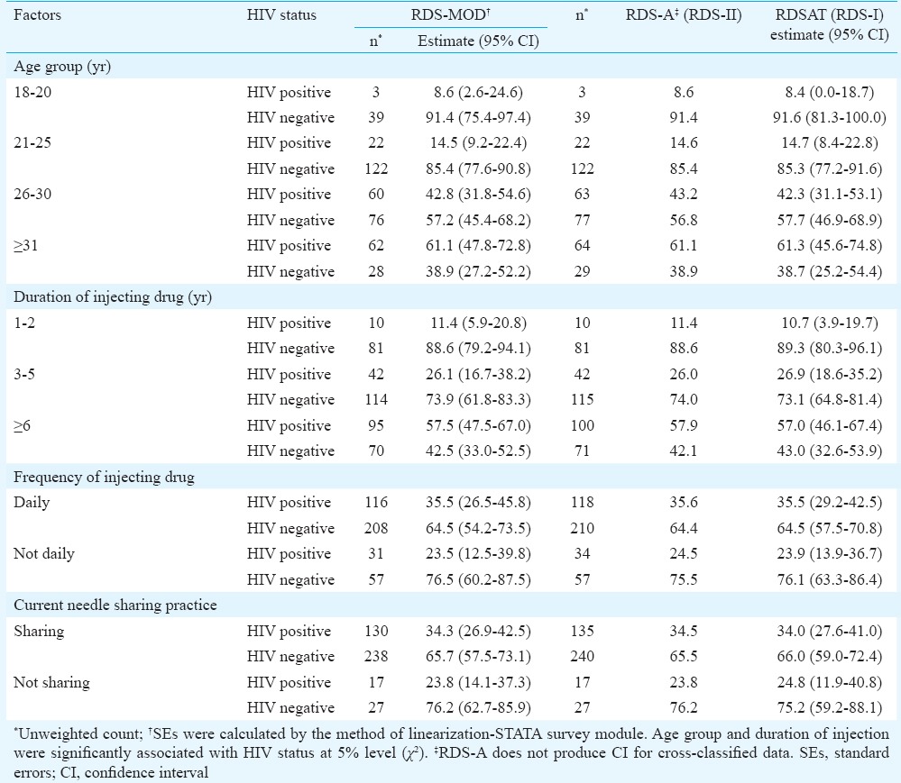
Table III.

Estimates of proportions [given as (estimates and 95% CI)] of various subgroup of variables using respondent-driven sampling (RDS)-MOD (modified), RDS-A (analyst) and respondent-driven sampling analysis tool (RDSAT) on different datasets, viz. faux, fauxsycamore, fauxmadrona

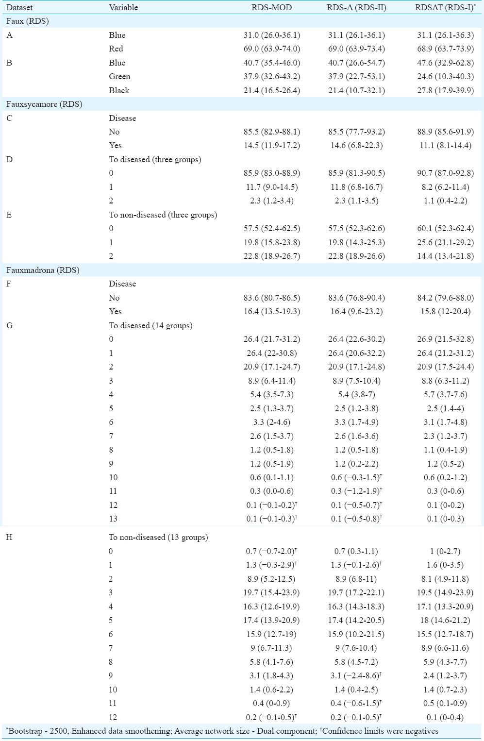
Table IV.

Estimates of proportions [estimates (95% CI)] using respondent-driven sampling (RDS)-MOD (modified), RDS-A (analyst) and respondent-driven sampling analysis tool (RDSAT) on Jazz musician datasets

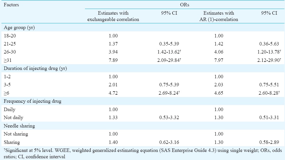
Regression analyses: Similarity induced by clusters would violate the standard assumption of independent observations from each individual. In the regression set-up, generalized estimating equation approach accounts for intra-cluster correlation28. This approach was used to study the affiliation factors for HIV positivity (factors associated with HIV) among the IDUs recruited in Churachandpur, India. Regression analysis was performed using WGEE approach with auto-regressive-1 (AR-1) correlation structure as logical ordering of recruitment was inevitably present in the RDS selection process. Furthermore, the AR-1 structure is appropriate when the correlation between various sample units is expected to decrease with the increasing distance within the recruitment chain. The CIs were obtained for the parameter estimates of regression equation by SAS software29. The results are presented in Table V. To understand the nature of linkages in the recruitments among IDUs with HIV status, WGEE with exchangeable correlation structure was also performed. If Hx is high for a variable, the parameter estimates with these two assumed correlation (AR-1 and exchangeable) structures would vary in the regression.

Table V.

Factors associated with HIV for different correlation structure of weighted generalized estimation equation

Results

The proposed weights were similar to RDS II of Volz and Heckathorn13 but for a constant term (harmonic mean of the network size) in the numerator as normalizing factor.

Comparison of estimates of parameters of different datasets by RDS-MOD with RDSAT and RDS-A

Churachandpur, India RDS data: All the seeds grew and reached up to seven waves. The recruitment per se ed ranged from 50 to 111. A random mixing pattern of recruitment was observed among HIV positives and negatives in the network recruitment diagram (Fig. 1A) and also in the demographically adjusted recruitment matrices of RDSAT (symmetry, not shown). Estimated waves required to reach equilibrium was 2-3 for all variables, except for only one subset variable. All the variables considered for this analysis attained equilibrium with more than six waves. RDSAT and RDS-A used all 419 recruits for analysis.

For our new approach (RDS-MOD), 17 clusters were formed after discarding six seeds (Fig. 1B). For example, when seed 2 was removed, three clusters were formed with assigned cluster numbers C4, C5 and C6 of size 41, 28 and 41, respectively. Only one cluster (C2) of size one from seed 1 was not considered for cluster analysis. Thus, 16 clusters of 412 recruits were available for analysis by our new approach with a loss of seven participants including, six seeds and one first-wave recruit.

Bland–Altman plots indicated that single weights of RDS-MOD and weights of RDSAT for different variables were within the acceptance limits (i.e. within the mean of differences of weights between these two methods ±1.96 of standard deviation of these differences) for all the four variables considered (Fig. 2). Further, the mean of the differences was nearly zero signalling that the single weight per participant was similar to multiple weights of RDSAT. However, the trends within them indicated that the differences varied with magnitude. Thus, the calculated weights by both methods depended strongly on each other. This indicated the reasonability between the weights calculated by our approach for an individual and several of RDSAT's weights for different variables of the same individual for this dataset.

The estimates of proportions by RDS-MOD across variables were similar to RDS-A and RDSAT (Table I). However, the CIs by RDS-MOD were wider compared to other two methods. The Hx was highest for the character ‘sharing of injection needle’ (Hx = 0.381). The other affiliation characters for HIV were ‘daily injection of drugs’ (Hx = 0.156) and ‘duration of injecting drugs more than five years’ (Hx = 0.143). Negative affiliation in the recruitment was noticed among those with duration of injecting drugs less than two years (Hx = −0.149). For a sub-sample, RDSAT produced estimates not in tune with the observed frequencies and RDSAT could not produce CI. For example, a random sample of 37 specimens was tested for herpes simplex virus type 2 (HSV- 2). Among them eight were ‘positive’, two were ‘inconclusive’ and the remaining ‘negative’. RDSAT estimated the proportions of positives (8 out of 37) as 0 per cent and inconclusive (2 out of 37) as 37.1 per cent. RDSAT showed that the estimated mean number of waves to attain equilibrium for this variable was as high as 1960 (Table I).

RDS-MOD yielded similar and comparable parameter estimates of cross-classified variables as well (Table II). However, slightly wider CI was noticed in many of the estimates by RDS-MOD both in Tables I and II. RDS-A did not produce CI for cross-classified data (Table II).

By RDS-MOD method, all parameters were re-estimated using individualized weights per variable generated by RDSAT (data not shown). The estimates were almost similar to that of single weighting procedure of RDS-MOD implying that single weight per individual was sufficient rather than multiple weights per individual. Similar exercise was performed on cross-classified data of parameters. The estimates by single weight approach and those with individualized weights of RDSAT were identical (data not shown). This also indicated that single weighting approach worked well for cross-classified estimations.

Comparison of results of RDS-MOD, RDSAT and RDS-A with other example datasets: The estimates of parameters and their CIs of the other example RDS datasets are presented in Tables III and IV. This exercise was done for not drawing any inference but to compare the estimates.

Dataset 1 – faux: From the faux dataset, the variable ‘A’, the estimates of population parameters by RDS-A (RDS II), RDS-MOD and RDSAT (RDS I) were almost similar including their CIs. However, for variable ‘B’ of the same datasets, population estimates by RDS-A and RDS-MOD were identical and RDSAT (RDS I) yielded varied results for all the three parameters.

Dataset 2 – fauxsycamore: For all the three variables (C, D, E), the estimates by RDS-MOD and RDS-A were comparable. The CIs produced by RDS-MOD were almost equal or narrower than RDS-A. RDSAT (RDS I) produced results differently for all these variables.

Dataset 3 – fauxmadrona: This dataset contains three variables (F, G, H). The variable ‘G’ has 14 groups and ‘H’ has 13 groups. The estimates by RDS-MOD and RDS-A were identical and the estimates by all the three methods were comparable. For ‘G’, the CIs were wider for RDS-A. RDS-MOD gave narrow CIs. RDS-MOD and RDS-A produced negative limits for some CIs. However, RDSAT did not produce any of that type.

Dataset 4 – Jazz musician: The estimates of parameters by RDS-MOD and RDS-A were identical. RDS-MOD yielded narrow CI. RDSAT also produced comparable results for all the four variables.

Dataset 5 – Bishnupur, Phek and Wokha: HIV prevalence estimate and CI was similar to RDS-A in Wokha and CI was slightly wider in Bishnupur data. However, CI of Phek data by RDS-MOD was wider (data not shown).

Results of regression analysis: WGEE both with AR-1 and exchangeable correlation structures showed that older age groups (≥25 yr) and longer period of injecting drug use (≥6 yr) were associated with HIV positivity (Table V). Sharing of needles daily was not associated with HIV positivity. The similarity of regression coefficients both by AR-1 and exchangeable correlation structure indicated the random mixing nature of HIV status of recruiter and recruits in Churachandpur data (Table V).

Discussion

As there is no method available to make the true estimate of the parameter of RDS data, all our comparisons were mainly with RDS II (this method calculates SEs of estimates analytically) estimates, and hence, the comparison of the RDS-MOD estimates with other methods such as successive sampling method was not possible. The proposed new approach for analysis of RDS data was simple and less time-consuming. Additionally, this approach was able to generate population estimates comparable to those derived by RDS-A (RDS II), the currently available most advanced level software to analyze RDS data. Precision of estimates by our approach appeared to be superior to RDS-A in the example datasets [viz. faux (RDS); fauxsycamore (RDS); fauxmadrona (RDS) and Jazz musicians dataset].

In the new approach, clusters were formed without affecting sequential and natural ordering of selection. In this process, though information on all seeds (non-random) was lost, RDS data were robust and not likely to be affected by the inclusion or exclusion of out of equilibrium data, i.e. data collected before reaching equilibrium30. Discarding of earlier waves has also been recommended in previous reports10,15. Thus, our result might not be affected by discarding the six seeds from the analysis. Formation of clusters paved a way to account for the related characters in the recruitment process and provided ways to other statistical methods and analysis by routine statistical software.

It has been suggested that the tendency towards Hx varies among groups31. Hence, it is important to measure the tendency towards Hx with respect to different respondent's characteristics and to use this information to weight the sample to compensate for any biases31. It appears that in general, the network's composition with respect to personal attributes may exhibit Hx with respect to only a particular trait or with respect to a few characters. In our sample, ‘sharing of needle’ was the most prominent trait (knowing each other) irrespective of the HIV status. Therefore, technically, a single unique weight would be sufficient to compensate the Hx of different respondent characteristics. In addition, as sampling weights were used only to compensate the unequal probability of inclusion into the sample, a common weight for each individual was sufficient rather than individualized weights for each variable and the results were comparable to those of RDSAT. The similarity of the parameter estimates by our approach using RDSAT weights in one-way and two-way tables indicated that a single weight per individual was sufficient.

Our RDS-MOD approach was similar to RDS II of Volz and Heckathorn6. The only difference was that the weights by RDS-MOD had an additional constant multiplier compared to Volz and Heckathorn. Although this constant does not affect the estimates, it is needed for the physical comparison of weights with that of RDSAT. The very basic assumption made was that a recruiter recruited the subjects independently with probability proportional to network size of the recruiter. This assumption was based on the work of Salganik and Heckthorn8, who showed that a random walk on network was a Markov Process, in which equilibrium occupied a node with probability proportional to degree. The applicability of Hansen-Hurwitz estimator with these assumptions provides theoretical and conceptual foundation to our approach of deriving unique weights32.

The proposed approach necessitated the need for incorporating clustering effect in the regression model as clustering results in lack of independence among the errors in regression. Generalized estimating equation (GEE) approach resolves this problem by appropriately accounting the correlation structure of a variable of interest between recruits and recruiter28. The process of fitting a model should incorporate sample weights as well as information about correlation between sample units. Weighted estimating equations are the most popular methods for obtaining consistent estimates of regression coefficient with sample survey data33,34. Therefore, we used WGEE approach to study the affiliation factors for the HIV positivity. AR-1 correlation structure accounted for logical ordering of recruitment and the exchangeable correlation assumed equality of correlation between any two recruited individuals within a cluster. The similarity of results due to different correlation structures (AR-1 and exchangeable) suggested that HIV status was not an indicative factor for recruitment preferences in recruiting HIV-positive/negative IDUs in Churachandpur dataset. Slight variations found in model coefficients by these two procedures (AR-1 and exchangeable) could be due to possible omission of a variable from the model that had a strong interaction with the independent variables and was highly correlated with the weights35.

The advantage of our approach is that it allows estimations using standard software such as STATA or any other software that accommodates survey sampling method. Also, the problem of subgroup analysis of RDS data could be overcome.

It was assumed that the clusters formed were independent after discarding a seed although some traits of that seed might prevail upon clusters of that seed. However, this limitation can be overcome by selecting more seeds at the stage of data collection (preferably independent) and considering each seed with its recruits as a separate cluster as has been done with other example datasets. The new approach resulted in slightly wider CIs in Churachandpur data compared to RDS-A and RDSAT. The possible reasons could be that RDS-MOD employed the analytical method to calculate these. It could also happen if the intra-cluster correlation was high. Volz and Heckathorn6 have reported that wider CI is expected when the variances are calculated analytically. Empirical tests of RDS have indicated that the analytical method overestimates the CIs30. As we have also accounted for the intra-cluster correlation, still wider CIs are expected36. Clustering and weighting normally result in decreased precision37. Volz and Heckathorn6 suggested that the loss of precision might happen due to the single weights used for all variables as was done in the present study. In contrast, RDS-MOD yielded estimates with the same or higher precision in other simulated example datasets, viz., faux (RDS); fauxsycamore (RDS) and fauxmadrona (RDS) and Jazz musicians dataset used for comparisons. This indicated the possibility that intra-cluster correlation in these example datasets (simulated data) was not high. As the inferences based on RDS data require many strong assumptions, Gile et al38 have suggested some diagnostic tools to empower researchers to understand their RDS data better and encourage future statistical research on RDS sampling and inference.

Our study had certain limitations. The weight calculation was solely dependent on the network size (degree reported by the respondent). Thus, inaccuracies in the self-reported degree might have introduced biases in the estimates. Hanzen-Hurwitz method is applicable only when the sample elements are selected independently with replacement and that may not be true in the real sense of RDS. We assumed that the clusters formed were independent though some traits of corresponding seed would have prevailed. A few of the lower limits of our CIs in an example dataset for proportions were negative.

In conclusion, the proposed alternative approach of using single weight and converting RDS data into clusters before analysis can be recommended as it generates analytical CIs and allows for estimates for smaller groups as well. RDS data can thus be analyzed faster using commonly used statistical software that also permits wider range of statistical analysis including analysis of continuous variables.

References

- 1.Goodman L. Snowball sampling. Ann Math Stat. 1961;32:148–70. [Google Scholar]
- 2.Deaux E, Callaghan JW. Key informant versus self-report estimates of health behavior. Eval Rev. 1985;9:365–8. [Google Scholar]
- 3.Watters JK, Biernacki P. Targeted sampling: options for the study of hidden populations. Soc Probl. 1989;36:416–30. [Google Scholar]
- 4.Heckathorn DD. Respondent-driven sampling: a new approach to the study of hidden populations. Soc Probl. 1997;44:174–99. [Google Scholar]
- 5.Singh P, Pandey A, Aggarwal A. House-to-house survey vs. snowball technique for capturing maternal deaths in India: a search for a cost-effective method. Indian J Med Res. 2007;125:550–6. [PubMed] [Google Scholar]
- 6.Volz E, Heckathorn DD. Probability based estimation theory for respondent-driven sampling. J Off Stat. 2008;24:79–97. [Google Scholar]
- 7.Fararo TJ, Skvoretz J. Biased networks and social structure theorems. Soc Networks. 1984;6:223–58. [Google Scholar]
- 8.Salganik MJ, Heckathorn DD. Sampling and estimation in hidden populations using respondent-driven sampling. Sociol Methodol. 2004;34:193–239. [Google Scholar]
- 9.Gile KJ, Handcock MS. Respondent-driven sampling: an assessment of current methodology. Sociol Methodol. 2010;40:285–327. doi: 10.1111/j.1467-9531.2010.01223.x. [DOI] [PMC free article] [PubMed] [Google Scholar]
- 10.Goel S, Salganik MJ. Respondent-driven sampling as Markov chain Monte Carlo. Stat Med. 2009;28:2202–29. doi: 10.1002/sim.3613. [DOI] [PMC free article] [PubMed] [Google Scholar]
- 11.Griffiths P, Gossop M, Powis B, Strang J. Reaching hidden populations of drug users by privileged access interviewers: methodological and practical issues. Addiction. 1993;88:1617–26. doi: 10.1111/j.1360-0443.1993.tb02036.x. [DOI] [PubMed] [Google Scholar]
- 12.Johnston LG, Malekinejad M, Kendall C, Iuppa IM, Rutherford GW. Implementation challenges to using respondent-driven sampling methodology for HIV biological and behavioral surveillance: field experiences in international settings. AIDS Behav. 2008;12:S131–41. doi: 10.1007/s10461-008-9413-1. [DOI] [PubMed] [Google Scholar]
- 13.Volz E, Wejnert C, Degani I, Heckathorn DD. Respondent-driven sampling analysis. RDSAT 6.01. Ithaca, NY: Cornell University; 2007. [Google Scholar]
- 14.Salganik MJ. Variance estimation, design effects, and sample size calculations for respondent-driven sampling. J Urban Health. 2006;83:i98–112. doi: 10.1007/s11524-006-9106-x. [DOI] [PMC free article] [PubMed] [Google Scholar]
- 15.Burt RD, Thiede H. Evaluating consistency in repeat surveys of injection drug users recruited by respondent-driven sampling in the Seattle area: results from the NHBS-IDU1 and NHBS-IDU2 surveys. Ann Epidemiol. 2012;22:354–63. doi: 10.1016/j.annepidem.2012.02.012. [DOI] [PMC free article] [PubMed] [Google Scholar]
- 16.Taran YS, Johnston LG, Pohorila NB, Saliuk TO. Correlates of HIV risk among injecting drug users in sixteen Ukrainian cities. AIDS Behav. 2011;15:65–74. doi: 10.1007/s10461-010-9817-6. [DOI] [PubMed] [Google Scholar]
- 17.Gile KJ. Improved inference for respondent-driven sampling data with application to HIV prevalence estimation. J Am Stat Assoc. 2011;106:135–46. [Google Scholar]
- 18.Heckathorn DD. Extensions of respondent-driven sampling: analyzing continuous variables and controlling for differential recruitment. Sociol Methodol. 2007;37:151–207. [Google Scholar]
- 19.Szwarcwald CL, de Souza Júnior PRB, Damacena GN, Junior AB, Kendall C. Analysis of data collected by RDS among sex workers in 10 Brazilian cities, 2009: estimation of the prevalence of HIV, variance, and design effect. J Acquir Immune Defic Syndr. 2011;57:S129–35. doi: 10.1097/QAI.0b013e31821e9a36. [DOI] [PubMed] [Google Scholar]
- 20.Salganik MJ. Respondent-driven sampling in the real world. Epidemiology. 2012;23:148–50. doi: 10.1097/EDE.0b013e31823b6979. [DOI] [PubMed] [Google Scholar]
- 21.Handcock MS, Fellows IE, Gile KJ. Software for the analysis of respondent-driven sampling data. Version 0.42. Los Angeles, CA: Hard to Reach Population Methods Research Group; 2014. [Google Scholar]
- 22.Shah VB. Linearization methods of variance estimation. In: Armitage P, Colton T, editors. Encyclopedia of Biostatistics. New York: John Wiley & Sons, Inc; 1998. pp. 2276–9. [Google Scholar]
- 23.Mahanta J, Medhi GK, Paranjape RS, Roy N, Kohli A, Akoijam BS, et al. Injecting and sexual risk behaviours, sexually transmitted infections and HIV prevalence in injecting drug users in three states in India. AIDS. 2008;22(Suppl 5):S59–68. doi: 10.1097/01.aids.0000343764.62455.9e. [DOI] [PubMed] [Google Scholar]
- 24.Chandrasekaran P, Dallabetta G, Loo V, Mills S, Saidel T, Adhikary R, et al. Evaluation design for large-scale HIV prevention programmes: the case of Avahan, the India AIDS initiative. AIDS. 2008;22(Suppl 5):S1–15. doi: 10.1097/01.aids.0000343760.70078.89. [DOI] [PubMed] [Google Scholar]
- 25.Volz E, Wejnert C, Cameron C, Spiller M, Barash V, Degani I, et al. Respondent-driven sampling analysis tool (RDSAT). Version 7.1. Ithaca, NY: Cornell University; 2012. [Google Scholar]
- 26.Altman DG, Bland JM. Measurement in medicine: the analysis of method comparison studies. Statistician. 1983;32:307–17. [Google Scholar]
- 27.StataCorp. Stata statistical software. Release 10. 10th ed. TX: StataCorp LP; 2007. [Google Scholar]
- 28.Liang KY, Zeger S. Longitudinal data analysis using generalized linear models. Biometrika. 1986;73:13–22. [Google Scholar]
- 29.SAS®. SAS-administering SAS® enterprise guide®. 4.3. Cary, NC: SAS Institute Inc; 2010. [Google Scholar]
- 30.Wejnert C. An empirical test of respondent-driven sampling: point estimates, variance, degree measures, and out-of-equilibrium data. Sociol Methodol. 2009;39:73–116. doi: 10.1111/j.1467-9531.2009.01216.x. [DOI] [PMC free article] [PubMed] [Google Scholar]
- 31.Heckathorn DD. Respondent-driven sampling II: deriving valid population estimates from chain-referral samples of hidden populations. Soc Probl. 2002;49:11–34. [Google Scholar]
- 32.Hansen M, Hurwitz W. On the theory of sampling from finite populations. Ann Math Stat. 1943;14:333–62. [Google Scholar]
- 33.Binder DA. On the variances of asymptotically Normal Estimators from Complex Surveys. Int Stat Rev. 1983;51:279–92. [Google Scholar]
- 34.Pfeffermann D. The role of sampling weights when modeling survey data. Int Stat Rev. 1993;61:317–37. [Google Scholar]
- 35.Korn EL, Graubard BI. Examples of differing weighted and unweighted estimates from a sample survey. Am Stat. 1995;49:291–5. [Google Scholar]
- 36.Pfeffermann D. The use of sampling weights for survey data analysis. Stat Methods Med Res. 1996;5:239–61. doi: 10.1177/096228029600500303. [DOI] [PubMed] [Google Scholar]
- 37.Dowd AC, Duggan MB. Computing variances from data with complex sampling designs. Comparison of STATA and SPSS. Boston: North American Stata Users Group; 2001. [Google Scholar]
- 38.Gile KJ, Johnston LG, Salganik MJ. Diagnostics for respondent-driven sampling. J R Stat Soc Ser A Stat Soc. 2015;178:241–69. doi: 10.1111/rssa.12059. [DOI] [PMC free article] [PubMed] [Google Scholar]