

Abstract
Purpose
Filter exchange imaging (FEXI) is sensitive to the rate of diffusional water exchange, which depends, eg, on the cell membrane permeability. The aim was to optimize and analyze the ability of FEXI to infer differences in the apparent exchange rate (AXR) in the brain between two populations.
Methods
A FEXI protocol was optimized for minimal measurement variance in the AXR. The AXR variance was investigated by test‐retest acquisitions in six brain regions in 18 healthy volunteers. Preoperative FEXI data and postoperative microphotos were obtained in six meningiomas and five astrocytomas.
Results
Protocol optimization reduced the coefficient of variation of AXR by approximately 40%. Test‐retest AXR values were heterogeneous across normal brain regions, from 0.3 ± 0.2 s−1 in the corpus callosum to 1.8 ± 0.3 s−1 in the frontal white matter. According to analysis of statistical power, in all brain regions except one, group differences of 0.3–0.5 s−1 in the AXR can be inferred using 5 to 10 subjects per group. An AXR difference of this magnitude was observed between meningiomas (0.6 ± 0.1 s−1) and astrocytomas (1.0 ± 0.3 s−1).
Conclusions
With the optimized protocol, FEXI has the ability to infer relevant differences in the AXR between two populations for small group sizes. Magn Reson Med 77:1104–1114, 2017. © 2016 The Authors Magnetic Resonance in Medicine published by Wiley Periodicals, Inc. on behalf of International Society for Magnetic Resonance in Medicine. This is an open access article under the terms of the Creative Commons Attribution‐NonCommercial‐NoDerivs License, which permits use and distribution in any medium, provided the original work is properly cited, the use is non‐commercial and no modifications or adaptations are made.
Keywords: diffusion MRI, filter exchange imaging, cell membrane permeability, study design
INTRODUCTION
Diffusion‐weighted imaging (DWI) probes tissue properties on the microscopic level 1. Physiologically important parameters such as the density and diameter of axons can be estimated by modeling the effect of the cellular environment on diffusion‐weighted data 2, 3, 4, 5. Such modeling generally assumes that water is confined within intra‐ and extracellular compartments, separated by cell membranes. However, water exchange takes place between the compartments, either directly through the lipid bilayer or facilitated through so‐called aquaporins (AQP) 6, 7. The exchange rate is proportional to the cell membrane permeability to water 8, 9, which is important for cell volume regulation 10 and for conditions involving edema such as tumors, infection, and stroke 11, 12. In aggressive tumors, AQP upregulation has been demonstrated 13, 14, 15. Quantification of exchange rates by MRI may yield a biomarker that is sensitive to alterations of cell membrane permeability, and offer improved diagnostics and more adequate treatment.
Conventional DWI is based on the single‐diffusion encoding (SDE) experiment, and the data acquired are typically analyzed by methods such as diffusion tensor imaging (DTI) or diffusion kurtosis imaging (DKI), which do not account for effects of exchange. It is possible to estimate the exchange rate of water between compartments using SDE by acquiring data using multiple diffusion times and applying a modified Kärger model 16, 17, 18. However, this approach has the limitation that the effects from exchange and restricted diffusion are entangled. With increased diffusion time, effects from exchange increase the attenuation for high b‐values, whereas effects from restriction reduce it 18. For higher specificity to exchange, a double‐diffusion encoding (DDE) sequence can be employed 9, 19. Filter exchange imaging (FEXI) is a DDE‐based method implemented for clinical use that yields the apparent exchange rate (AXR) 20. The advantages of estimating AXR rather than using the Kärger model were discussed previously 20.
The AXR is sensitive to changes in membrane permeability 9, 20, and has been measured in the healthy human brain and a meningioma brain tumor 21. In fixed monkey brain, a tensor‐based AXR analysis has been explored 22. Preliminary data showed that the AXR is sensitive to altered gene expression of the urea transporter 23. The FEXI method has also been applied to investigate breast tumor cells 24. The FEXI method has great promise, but its reproducibility in a clinical setting has not yet been studied. In this study, we aimed to optimize and analyze the ability of FEXI to infer differences in the AXR in the brain between two populations in clinical studies. We took three steps to meet this aim. First, we optimized a FEXI protocol for minimal AXR variance caused by measurement noise. Second, we investigated the AXR variance in the normal brain by performing a test‐retest study on healthy volunteers, using the optimized protocol. Third, we obtained FEXI data from patients with meningiomas and astrocytomas to demonstrate that the AXR is sensitive to their microstructural differences 25.
THEORY
Filter Exchange Imaging
The FEXI pulse sequence is illustrated in Figure 1. It is based on a stimulated‐echo DDE sequence with two pulsed gradient spin‐echo (PGSE) blocks separated by a mixing time (t m) and followed by an echo‐planar imaging (EPI) block. The diffusion weighting factor (b) of the PGSE blocks is given by b = (γgδ)2 t d, in which γ is the nuclear gyromagnetic ratio and t d is the effective diffusion time (t d = Δ – δ/3) of the gradient pairs with amplitude g, duration δ, and separation between the leading edges Δ, and correspondingly for the b‐value of the first block (b f).
Figure 1.
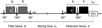
Illustration of the FEXI pulse sequence. FEXI employs a stimulated echo DDE sequence. The two diffusion‐encoding blocks, the “filter” and the “detection” block, have gradient strengths g, diffusion weightings b f and b, and gradient timing parameter pairs (Δf, δf) and (Δ, δ), respectively. The magnetization is stored longitudinally during the mixing time (t m) by the second 90° pulse, and then refocused by a third 90° pulse. Spoiler gradients dephase the magnetization excited by the extra 90° pulses. After the detection block, the signal is acquired by echo‐planar imaging (EPI, with readout time τEPI).
To derive the FEXI model 20, we assume that water exists in two compartments with approximately Gaussian diffusion and equal longitudinal and transversal relaxation rates, but different apparent diffusivities, denoted as “slow” (D s) and “fast” (D f), respectively. Water molecules in the slow and fast compartments contribute with equilibrium fractions of the MR signal ( and ), where + = 1. In the presence of diffusion‐encoding gradients, the signal attenuation in each compartment is determined by its apparent diffusion coefficient (ADC). In FEXI, the diffusion weighting of the first PGSE block (the “filter block”) will therefore preferentially attenuate, or “filter out,” the signal from the fast compartment, which results in apparent signal fractions that are perturbed from equilibrium ( > and < ). During the mixing time, exchange takes place between the compartments, which at t m will have restored toward according to
| (1) |
where k sf and k fs are the forward and reverse exchange rates between the slow and the fast compartment, and (0) is the fast fraction immediately after the filter 9. Due to mass balance, k sf and k fs are related to the fractions according to f s k sf = f f k fs. The durations of the diffusion‐encoding blocks are assumed to be short enough for significant exchange to take place only during t m 9. The diffusion weighting of the second PGSE block (the “detection block”) is used to estimate the ADC, which depends on the fractions, and thus t m, according to
| (2) |
Rather than using the Kärger model to obtain D s, D f, , , and the exchange rate k = k sf + k fs 9, FEXI measures the response to t m in the initial, approximately monoexponential, decay of the signal. This decay is proportional to ADC'(t m), which is given by
| (3) |
where ADC is the apparent diffusion coefficient at equilibrium, σ = 1 – ADC'(0)/ADC is the filter efficiency, and AXR is the apparent exchange rate. In a two‐compartment system, AXR = k. In a multicompartment system, the AXR approximates the “mean exchange” in a similar way to how the ADC approximates the “mean diffusivity” 20. The MR signal at t m is given by
| (4) |
where S 0(t m) is the relaxation‐weighted signal without diffusion encoding 21. The minimal sampling requirement to fit Eq. (4) and estimate ADC, σ, and AXR is a combination of two different b with two different t m. Additionally, ‘unfiltered’ data acquired with b f = 0 must be obtained for some number of t m to estimate the equilibrium ADC.
Statistical Power and Parameter Variance
We describe two concepts related to the analysis of the test‐retest data: analysis of statistical power, and partitioning variance contribution between intersubject differences within the population and measurement noise.
The power of a statistical test (π) that compares a parameter between two groups is the probability of the test to find an effect with significance (α) in the presence of a true difference. It depends on the effect size (such as a difference in means, Δμ), the variance of parameter observations (V), and the group sizes (n, assuming they are equal). In the analysis of statistical power, any of these quantities (α, π, Δμ, V, and n) can be calculated for a given type of test by fixing the values of the others 26. This is useful in study design to ensure that group sizes are sufficiently large to assess an effect of known (or hypothesized) size.
In a population, the variance of parameter observations depends on both the intersubject variance (V I) about the population mean (μ), and on the variance introduced by measurement noise (V M). In a two‐level random effects model for an observation Y ij on subject i ∊ [1…I], in the repeated measurement j ∊ [1…J], this is expressed as
| (5) |
where ε i and ε j are the subject and measurement level errors, respectively 27. The total variance is V = Var(Y ij) = Var(ε i) + Var(ε j) = V I + V M, assuming Cov(ε i, ε j) = 0. Provided data from at least two measurements (J > 1), both V I and V M can be estimated. The relative variance contribution from measurement noise may then be estimated as RV M = V M/(V I + V M) = V M/V 28. It is a measure of the degree to which statistical power can be increased, and the required group sizes minimized, through experimental improvements such as protocol optimization.
METHODS
Protocol Optimization
We aimed to optimize a FEXI protocol for minimal variance in AXR caused by measurement noise (V M). To reach this aim, we followed the concepts introduced by Alexander 29, and minimized an objective function based on the Cramér‐Rao lower bound (CRLB) of the AXR. For estimates of a given model parameter in an unbiased model, the CRLB is a lower bound for V M 30, 31. It is expressed analytically based on the signal model (Eq. (4) for FEXI), a noise model, and the experimental protocol. In the following, we describe two aspects of our approach: the FEXI protocol and the CRLB‐based protocol optimization.
The FEXI protocol
With “protocol” we refer to the set of values for experimental parameters used during acquisition, such as the filter strength (b f), the detection b‐value (b), and the mixing time (t m). In our implementation, the acquisition loop obtains all detection b‐values and diffusion‐encoding directions for all mixing times, in which at least one mixing time is unfiltered (b f = 0). In the optimization, we simplified the protocol by considering only two different b and t m. This approach is unlike that of the previously presented protocol, which used a range of t m 21. We also fixed the values of the short t m ( = 16 ms) and the low b (b min = 40 s/mm2), to maximize the signal‐to‐noise ratio (SNR) while allowing the spoiling of unwanted echoes. The unfiltered acquisitions always used the shortest t m to maximize the SNR.
The parameters left to the optimization were b f, the high b (b max), the long t m ( ), the number of repetitions at the low and high b (#b min and #b max), the number of repetitions at the short and long t m (# and # ), and the number of unfiltered mixing time repetitions (# ). In addition, the maximal gradient amplitude (g) and the EPI readout time (τ EPI) were kept free, yielding a total of 10 optimization parameters. The effective number was nine, however, due to the following relation: Taq/TR = n dir(#b min + #b max)(# + # + # ), where Taq is the acquisition time, n dir is the number of diffusion‐encoding directions, and TR is the repetition time. The full set of optimization parameters is presented in Table 1, with allowed intervals. The upper limits for b and b f were set to 1300 s/mm2 to comply with the FEXI method of observing the initial decay of the signal‐to‐b curve. The upper limit for g (80 mT/m) reflects the constraints of the testing system. Other constraints were Taq ≤ 15 min, n slice = 7, and n dir = 6.
Table 1.
Optimization Parameters of the FEXI Protocola
| Parameter | Interval | Optimum |
|---|---|---|
| b f (s/mm2) | 200−1300 | 830 |
| b max (s/mm2) | 200−1300 | 1300 |
| (ms) | 200−800 | 442 |
| #b min | 1−10 | 3 |
| #b max | 1−10 | 6 |
| # | 1−10 | 2 |
| # | 1−10 | 2 |
| # | 1−10 | 1 |
| g (mT/m) | 40−80 | 80 |
| τEPI (ms) | 30−100 | 63 |
| Taq (s) | ≤900 | 780 |
| n dir | 6 | |
| n slice | 7 |
The FEXI optimization parameters, together with some constraint parameters (Taq, n dir, n slice), are presented with allowed intervals and found optima. The optimized protocol reduced the CV of the AXR by approximately 40%, compared with the previously presented protocol 21, corresponding to a more than 60% reduction in Taq. Main differences include using only two different t m and a higher b max. The most important hardware limitation was the maximal gradient amplitude (g).
Note: b f, filter strength; b max, high detection b‐value; , long mixing time; #b min/max, number of repetitions at b min/max; # , number of repetitions at ; # , number of mixing time repetitions in which b f = 0; g, maximal gradient amplitude; τ EPI, EPI readout time; Taq, acquisition time; n dir, number of diffusion‐encoding directions; n slice, number of slices.
CRLB‐Based Optimization
To optimize the protocol, we constructed an objective function based on the coefficient of variation (CV) of the AXR (CV = /AXR), and used the CRLB of the AXR to approximate V M. The CRLB is obtained from the Fisher information matrix (F), which, assuming a Gaussian noise distribution, has the elements
| (6) |
corresponding to the model parameters m i and mj. Here, σn is the noise standard deviation and S k is the predicted signal for the kth set of protocol parameters (Eq. (4)). The CRLB of model parameter m i is the ith diagonal element of the inverse F: CRLBi = (F ‐1)ii 29.
The assumption of Gaussian noise in Eq. (6) is valid for SNR values above ∼2 32. To avoid protocols yielding an SNR near this limit, we introduced a penalty factor based on the minimum SNR of all measurement points (SNRmin), according to f P = 1 + ( − 1) · (1 + exp[α (SNRmin − SNRtol)])−1, where α = 6, = 10 and SNRtol = 3.
The full objective function was obtained by averaging the SNR‐penalized CV estimate over priors calculated from the two‐compartment exchange model 33 (D s, D f, f f, and the exchange time τi = 1/k sf) according to
| (7) |
The interval for the exchange time was postulated, τi ∊ [1.0, 4.0] s, whereas the other priors were based on previous studies of white matter 34, 35, 36: D s ∊ [0.1, 0.3] µm2/ms, D f ∊ [0.9, 1.3] µm2/ms, and f f ∊ [0.4, 0.7].
In the calculations, the SNR of the nondiffusion‐encoded signal (S 0 in Eq. (4)) was set to a reference value (SNRref = 40) and rescaled based on departures from corresponding reference values of the echo times of the filter and detection blocks (TEfref = 39 ms and TEref = 53 ms), the repetition time (TRref = 2500 ms), and the EPI readout time (τ EPIref = 63 ms) 21. The scaling was given by
| (8) |
where
| (9) |
| (10) |
| (11) |
The relaxation time constants were given fixed values, T 1/T 2 = 700/50 ms/ms, which were both low compared with values reported in white matter 35, 37, 38, but chosen to err on the safe side of low SNR (FEXI loses SNR for short T 1 due to relaxation during t m). Calculation of the echo times were based on g and τ EPI, according to TEf = 2[δ f(g,b f) + τRF] for the filter block with gradient duration δ f, and TE = 2[δ(g,b) + τRF + (HF – 0.5) τ EPI] for the detection block with gradient duration δ. Here, τRF is the duration of the inversion pulse (8 ms) and HF is the half scan factor (0.7). The repetition times were calculated as TR = t m n slice + TR0, where TR0 = n slice(TEf + TE) ≥ 33g. The last inequality modeled duty‐cycle restriction and had to be incorporated to execute the protocol with our software implementation. Improving the implementation may make it less restrictive.
The objective function was minimized using the stochastic self organizing migrating algorithm (SOMA, http://www.ft.utb.cz/people/zelinka/soma/). SOMA randomizes a population of guess vectors of the optimization parameters, based on their allowed intervals. A number of “migrations” are performed, in which the best guess (according to the objective function) is identified as the “leader,” toward which the rest of the population performs randomized steps (migrations). SOMA was executed six times with default settings, but with 100 migrations for a population size of 18, after which the best protocol was chosen.
To assess the optimization yield, we considered the ratio of the CRLB‐based CV estimate of the optimized protocol versus that of the previously presented protocol 21. Seeing that the protocols had different Taq, the ratio was corrected with ( / )1/2, using SNR ∝ (Taq)1/2. The obtained metric corresponds to the change in CV assuming equal Taq.
Methodological Validations
We validated the CRLB‐based CV estimate by comparing it with the CV estimated in a simulation procedure. A synthetic data set of 104 samples was created by adding Rice‐distributed noise to the signal (Eq. (4)) using a fixed SNR. The AXR standard deviation was then estimated from the set of AXR values obtained by fitting the model to each of the samples. The comparison was performed for AXR ground‐truth values between 0.1 and 5.0 s−1, whereas the other model parameters were fixed (ADC = 0.7 μm2/ms and σ = 0.3).
It is well known that ADC is optimally estimated using only two b‐values 39. Here, this was assumed also for t m in AXR estimation, as it can be seen as a series of exponential fits using first b and then t m. We tested the assumption by studying how the objective function was affected when protocols were modified to include a third mixing time ( ).
To assess the importance of the gradients for the optimal protocol, we also executed the full optimization procedure with an upper limit of g of 40 mT/m. Furthermore, to examine the sensitivity of the optimized protocol to changes in parameter values, we studied how the objective function (Eq. (7)) changed over the optimization ranges of b f and b max (Table 1).
FEXI Acquisition and Postprocessing
FEXI data were acquired on a Philips Achieva 3 Tesla (T) system (Amsterdam, Netherlands), equipped with 80 mT/m gradients with a maximum slew rate of 100 mT/m/ms on axis and an eight‐channel head coil, using the sequence implementation of Nilsson et al 21 and the optimized protocol. Seven contiguous axial slices were obtained at the spatial resolution of 3 × 3 × 5 mm3, with TEf/TE/TR = 39/66/2000 ms/ms/ms, yielding Taq = 13 min. The timing parameters of the filter and detection blocks were δf/δ = 11/10 ms/ms and Δf/Δ = 31/31 ms/ms.
Data were obtained from 18 healthy volunteers (9 male, 9 female, age 30 ± 7 years, mean ± standard deviation), a group of 6 meningioma patients (all female, age 59 ± 5 years), and a group of 5 astrocytoma patients (4 male, 1 female, age 45 ± 11 years). All tumor patients were scanned before surgical excision. In the volunteers, FEXI data were obtained twice in the same session to assess the test‐retest variability. Additionally, we acquired whole‐brain DTI data, fluid‐attenuated inversion recovery (FLAIR), and T1‐weighted (T1W) images. The FLAIR and T1W images were coregistered to the FEXI data using the Elastix software package 40, 41. The study was approved by the Regional Ethical Review Board at Lund University, and all subjects gave written informed consent.
The FEXI image volumes were corrected for motion and eddy currents with Elastix, using an extrapolation‐based approach 42. To ensure a rotationally invariant metric, the data were averaged arithmetically across the diffusion‐encoding directions before model fitting. Previous papers on exchange imaging have used either geometric averaging 21, 43, which is more sensitive to noise than the arithmetic average, or a tensor‐based approach 22, which demands higher SNR than available at our clinical scanner. For region of interest (ROI) based analysis, the signal vectors were also averaged across the ROI voxels. Maps of the FEXI model parameters were obtained by fitting Eq. (4), and keeping S 0 as a free parameter for each t m.
Test‐Retest Study
In the analysis, the test‐retest data were obtained from six ROIs defined manually on directionally encoded color (DEC) maps. The ROIs are illustrated for one volunteer in Figure 2, and were positioned in the anterior corona radiata (ACR), the anterior limb of the internal capsule (ALIC), the genu and splenium of the corpus callosum (CC), the cerebrospinal tract (CST), the lentiform nucleus (LN), and the thalamus (TH). Regional specificity took precedence over ROI volume. ADC, σ, and AXR were estimated in the ROIs and described with respect to mean and standard deviation, calculated from all 2 × 18 measurements. Additionally, for the AXR, the CV was calculated and the paired test‐retest data were used to calculate RV M. Finally, for each ROI and multiple AXR effect sizes, the estimated V of AXR estimates were used to calculate the group sizes required to achieve a statistical power of 0.8 at α = 0.05. In this calculation, we assumed groups with equal n and V.
Figure 2.
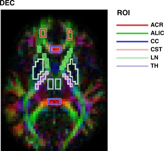
The six ROIs used in the test‐retest study, with data from one volunteer. ROIs were defined manually on DEC maps: the anterior corona radiata (ACR, dark red), the anterior limb of the internal capsule (ALIC, dark green), the genu and splenium of the corpus callosum (CC, dark blue), the cerebrospinal tract (CST, light red), the lentiform nucleus (LN, light green), and the thalamus (TH, light blue).
Intracranial Tumor Study
The solid part of each tumor was defined manually on the ADC map, guided by the coregistered T1W and FLAIR images. ROI volumes were between 57 and 179 voxels for meningiomas and 29 and 150 voxels for astrocytomas. ADC, σ, and AXR were estimated in each ROI and compared between the tumor groups using the Student's t‐test and the Mann‐Whitney U‐test (both Bonferroni corrected for the three comparisons).
After surgical excision, the specimens were paraffin‐embedded and fixed in 4% buffered formaldehyde solution. Sections of 4 μm were stained with hematoxylin‐eosin for visualization of tissue structure and cell morphology. The tumors were assessed neuropathologically, and microphotos were obtained from the specimens using an Olympus BX50 (Tokyo, Japan).
RESULTS
Protocol Optimization
The optimized protocol is presented in Table 1. Compared with the protocol used by Nilsson et al 21, the CV of the AXR was reduced by approximately 40%, assuming equal Taq. Noteworthy changes include the use of only two different t m (16 and 442 ms) rather than including a range of intermediate values, and using a higher b max (increased from 900 to 1300 s/mm2) 21. The optimized protocol featured the upper limit for b max and for the maximal gradient amplitude g (80 mT/m).
Methodological Validations
Figure 3a compares the CRLB‐based CV estimate (black) to the simulated CV (red). The CRLB‐based estimate yielded a negligible overestimation for AXR < 2 s−1, and a moderate underestimation for AXR between 3–5 s−1, but overall the two metrics showed good agreement.
Figure 3.
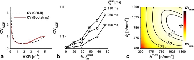
(a) Validation of the CRLB‐based CV estimate (black) by comparison with the CV estimated in a simulation experiment (red). The values for ADC and σ were fixed (ADC = 0.7 μm2/ms and σ = 0.3). The CRLB‐based estimate yielded a moderate underestimation for AXR values between 3 and 5 s−1, but was generally accurate. (b) Validation of the assumption that using only two different t m is optimal for AXR estimation. The curves show how the CV of the AXR was affected when the optimized protocol was altered to obtain different percentages of samples at a third mixing time ( ). For each value of , the CV increased monotonically with increased time spent sampling it. (c) Investigation of the performance sensitivity of the optimized protocol to changes in b f and b max. The objective function (Eq. (7)) was plotted over the ranges used in the optimization. The labeled contours show the percentage increase in CV from the optimized protocol (star).
The rationale for using only two different mixing times is shown in Figure 3b, where the CV of the AXR of a modified protocol is plotted against the percentage of samples obtained with . For all investigated protocols, we observed that adding samples at any leads to an increased CV.
In the optimization executed with a reduced upper limit of g (40 mT/m), the obtained protocol still featured the maximal allowed value of g, whereas settled at a slightly lower value of 378 ms, and b f and b max were reduced to 660 and 1100 s/mm2, respectively. Also, TEf and TE increased by 30 and 20%, respectively, and the CV almost doubled as a consequence.
Figure 3c shows the change of the objective function (Eq. (7)) over the optimization ranges of b f and b max. The labeled contours show the percentage increase compared with the optimized protocol (marked by a star). CV changes were small (<10%) for b f ∊ [600, 950] s/mm2 and b max ∊ [1000, 1300] s/mm2.
Test‐Retest Study
Figure 4 shows maps of ADC, σ, and AXR from one of the volunteers. The AXR map exhibits a heterogeneous contrast in the brain that was seen in many of the volunteers, including the previously observed distinctively high values in the frontal white matter 21. The test‐retest results for the parameters are presented in Table 2, with ROI means and standard deviations, and values of CV and RV M for the AXR. The mean AXR values varied substantially across the ROIs, being high in the ACR, intermediate in the TH, the LN and the ALIC, and low in the CST and the CC. The AXR estimates exhibited relatively high values of the CV, with a median of 41%. Values of RV M were also high, meaning that most of the variance was induced by the measurement rather than from the population. The observed test‐retest repeatability of the AXR is illustrated in Figure 5 by a scatter plot (left) and a Bland‐Altman plot (right), with test‐retest data pairs color‐coded by ROI. The scatter plot shows AXRtest versus AXRretest, which were clustered by ROI and correlated well. In the Bland‐Altman plot, the test‐retest AXR difference is plotted against the test‐retest AXR mean. A significant test‐retest bias was observed in the ACR (12%, Bonferroni corrected for the six comparisons).
Figure 4.
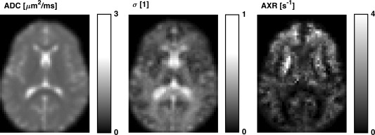
Maps of the FEXI model parameters ADC, σ, and AXR from one volunteer, all gamma corrected with γ = 0.7. The σ parameter is the filter efficiency, which shows the degree to which ADC is reduced by the action of the filter block. The heterogeneous contrast in the brain of the AXR map exemplifies the maps seen in the volunteers, including the distinctively high values in the frontal white matter observed previously 21.
Table 2.
FEXI Test‐Retest Results In the 18 Healthy Volunteersa
| ROI | ADC (μm2/ms) | σ | AXR (s−1) | CVAXR (%) | (RV M)AXR (%) |
|---|---|---|---|---|---|
| ACR | 0.7 ± 0.1 | 0.3 ± 0.1 | 1.8 ± 0.3 | 14 | 60 |
| ALIC | 0.6 ± 0.1 | 0.3 ± 0.1 | 0.9 ± 0.3 | 35 | 70 |
| CC | 0.7 ± 0.1 | 0.4 ± 0.1 | 0.3 ± 0.2 | 78 | 68 |
| CST | 0.6 ± 0.1 | 0.3 ± 0.1 | 0.4 ± 0.1 | 32 | 100 |
| LN | 0.7 ± 0.1 | 0.1 ± 0.1 | 1.2 ± 0.6 | 46 | 76 |
| TH | 0.8 ± 0.1 | 0.2 ± 0.1 | 0.8 ± 0.4 | 47 | 78 |
Shown for the 2 × 18 measurements are the ADC, sigma, and AXR (mean ± standard deviation) along with the CV and the RVM for the AXR. The AXR values were heterogeneous across the ROIs, and particularly high in the ACR.
Note: ACR, anterior corona radiata; ALIC, anterior limb of the internal capsule; CC, genu and splenium of the corpus callosum; CST, cerebrospinal tract; LN, lenticular nucleus; TH, thalamus.
Figure 5.
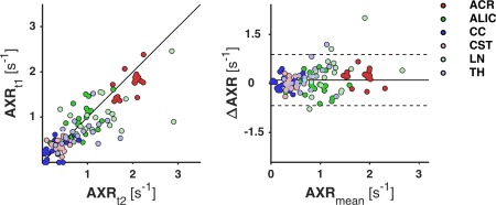
Illustration of the test‐retest repeatability of the AXR in the 18 healthy volunteers, by a scatter plot (left) and a Bland‐Altman plot (right). Test and retest AXR are denoted as AXRt1 and AXRt2, respectively; AXRmean is their mean; and ΔAXR is AXRt2 − AXRt1. In the scatter plot, the line corresponds to zero test‐retest difference, and in the Bland‐Altman plot, the lines denote the mean (solid) and limits (dashed) of a 95% confidence interval for AXR test‐retest differences, taken across all ROIs and all subjects. The dots are test‐retest data pairs, color‐coded by ROI. The plots (approximately) illustrate the measurement variance by distances of points to the middle lines, intersubject variance by spread of same‐colored points, and across‐ROI variance by spread of clusters of different‐colored points. The points show good correlation and are clustered by ROI. A significant test‐retest bias was observed in the ACR (12%).
Analysis of statistical power indicated that, in a ROI analysis, group mean differences in the AXR of 0.3–0.5 s−1 can be inferred using groups of 5 to 10 subjects per group. This was true for all investigated brain regions barring the LN, which showed higher variance.
Intracranial Tumor Study
Figure 6 shows FEXI parameter maps for each subject in the meningioma and the astrocytoma groups, together with coregistered T1W and FLAIR images. The meningiomas exhibited homogenously low AXR values, with the clear exception of case (f), which we considered to be an outlier. This case exhibited similar values of ADC and σ compared with the other meningiomas, although parts of it exhibited a darker FLAIR contrast, a feature that was also observed in parts of cases (a) and (c). This last finding may be explained by a T 2 reduction caused by a more fibrous content. In the AXR maps of the astrocytomas, the AXR was elevated compared with the normal appearing brain, and the elevation seemed correlated with the tumor outline in the T1W and FLAIR images. The FEXI parameters obtained in solid parts of the tumors are given in Table 3. The meningiomas exhibited low AXR values (0.6 ± 0.1 s−1, mean ± standard deviation), excluding the outlier for which AXR = 1.7 s−1. The AXR values of astrocytomas (1.0 ± 0.3 s−1) were significantly higher according to both the t‐test and the U‐test (ΔμAXR = 0.4 s−1, CI95 = [0.2–0.6] s−1, P < 0.05). The astrocytomas also exhibited significantly higher ADC values (1.2 ± 0.2 µm2/ms) compared with the meningiomas (0.8 ± 0.1 µm2/ms).
Figure 6.
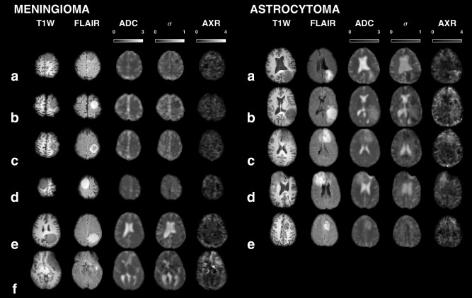
Overview of the FEXI parameter maps in the six meningioma and five astrocytoma patients, together with coregistered T1W and FLAIR images, all gamma‐corrected with γ = 0.7. The AXR values of the meningiomas were homogenously low (mean ± standard deviation, 0.6 ± 0.1 s−1), excluding the meningioma outlier case (f) in which AXR = 1.7 s−1. The astrocytomas exhibited significantly higher AXR values (1.0 ± 0.3 s−1) and ADC values (1.2 ± 0.2 versus 0.8 ± 0.1 µm2/ms). The outlier exhibited similar ADC and σ to the other meningiomas, although parts of it, and parts of cases (a) and (c), exhibited a darker FLAIR contrast, which could be caused by a more fibrous content.
Table 3.
FEXI Parameter Values In Meningiomas and Astrocytomasa
| Group | n | ADC (μm2/ms) | σ | AXR (s−1) | CVAXR (%) |
|---|---|---|---|---|---|
| meningioma | 6 | 0.8 ± 0.1b | 0.2 ± 0.1 | 0.8 ± 0.4 | 58 |
| meningioma* | 5 | 0.8 ± 0.1c | 0.2 ± 0.1 | 0.6 ± 0.1d | 20 |
| astrocytoma | 5 | 1.2 ± 0.2b, c | 0.2 ± 0.1 | 1.0 ± 0.3d | 26 |
FEXI parameter values are presented, with group means and standard deviation, for the meningioma group (six patients, grade I) and the astrocytoma group (five patients, grade II–IV). The meningioma* group is the meningioma group with one outlier excluded.
astrocytoma versus meningioma, P < 0.05, CI95% [0.3 0.6].
astrocytoma versus meningioma*, P < 0.05, CI95% [0.2 0.7].
astrocytoma versus meningioma*, P < 0.05, CI95% [0.2 0.6].
Tumor specimen microphotos are showed in Figure 7. In the neuropathological assessment, the meningioma specimens were classified as grade I 44 with varying histopathological types, including fibroblastic, syncytial, and transitional. The outlier meningioma, case (f), was of a transitional type and exhibited microscopic signs of increased growth potential, bringing it close to grade II (atypical). The astrocytoma specimens were classified as grade II–IV 44, and were heterogeneous with respect to cell density and signs of increased malignancy. In general, the meningiomas exhibited a dense growth pattern with high tissue cohesion and structures such as sheets and bundles, and often contained elongated cells. In contrast, the astrocytomas exhibited a looser, more homogeneous tissue structure, and showed no obvious anisotropy on the cellular scale.
Figure 7.
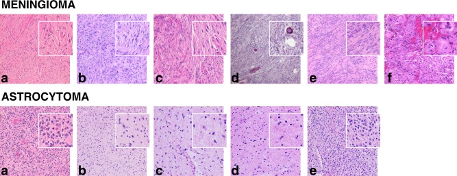
Microphotos of specimens of the surgically excised tumors. The meningiomas were grade I and had different histopathological types: fibroblastic in cases (a), (b), (d), and (e), fibroblastic/syncytial in case (c), and transitional in case (f). The outlier meningioma case (f) was close to grade II, as it exhibited microscopic signs of increased growth potential, such as slight nuclear atypia and pleomorphism, and incipient necroses. The astrocytomas were of different grades: IV in case (a) and (b), II and III in case (c) and (d), and II in case (e). They exhibited different degrees of cell density and signs of increased malignancy, such as high mitotic activity, vascular proliferation, and necrosis. The main histopathological difference between the tumor types was a denser and more cohesive tissue structure of meningiomas and the presence of elongated cells and structures such as sheets or bundles.
DISCUSSION
FEXI employs DDE for measuring the AXR, a quantity that cannot be estimated using ordinary DWI methods, such as DTI or DKI. In this work, the FEXI protocol was optimized for minimal AXR variance in the normal brain.
The optimized protocol, presented in Table 1 and also in 45, reduced the CV of the AXR by approximately 40%, compared with the previously presented protocol 21, corresponding to a reduction of more than 60% in Taq. Further reduction of variance and/or Taq can be achieved by technological improvements. The most important limiting hardware factor in the optimization was the maximal gradient amplitude (g), which attained its upper limit (80 mT/m) despite accounting for a duty‐cycle limitation by increasing TR linearly with g. Minimizing TE by using stronger gradients thus increases the SNR more effectively than minimizing TR to obtain more samples, at least for an assumed T 2 of 50 ms. Systems with stronger gradients are available at some sites, eg, 300 mT/m at the human connectome scanner 46.
For performing FEXI on systems with different hardware configurations, we recommend using the protocol in Table 1 with small modifications. A change in the SNR, eg, from using a coil with more channels (which was eight in this study), should not affect the optimal protocol, provided that the noise distribution remains approximately Gaussian (SNR > 2). A change in the available sampling time, such as an increased Taq or a reduced n slice, can be accommodated by adding extra samples while preserving the ratios #b min/#b max and # /# . A change in g, however, would affect TEf and TE, and possibly the optima for b f and b max. We make two points concerning this matter. First, we do not recommend breaking the upper b‐value limit (1300 s/mm2) due to the bias it may cause in the FEXI model. Second, the optimization performed with a halved upper limit of g (40 mT/m) reduced the optimal values for b f and b max by approximately 200 s/mm2. As illustrated in Figure 3c, b‐value reductions of this magnitude, alone, have only a small effect on the CV. Therefore, we conclude that most clinical systems should get near‐optimal performance using slightly reduced values for b f and b max.
When performing FEXI on other organs than the brain, new optimizations, including whether to use more than two mixing times, are necessary to account for differences in tissue priors and relaxation properties. Preliminary results using a FEXI protocol optimized for the breast has already been presented 24. Generally, faster exchange demands shorter mixing times, and vice versa, due to the exponential coupling of AXR and t m (Eq. (3)). This is illustrated by the valley shape of the CV in Figure 3a. The valley can be seen as a “measurement window,” in which the timescales of the system (the exchange time, τi) and the measurement (t m) are well matched. Choosing the proper t m moves the window to the AXR range of interest.
In the test‐retest study, the AXR was highest in the ACR and lowest in the CC, which also exhibited the highest CV values. In periventricular structures such as the CC, the AXR could be negatively biased by partial volume effects with cerebrospinal fluid (CSF) 21. Over all regions, the CV values of the AXR ranged between 14 and 78%. This is relatively large compared with other high b‐value techniques, such as diffusion kurtosis imaging (DKI), in which the CV is 4–8% for mean diffusivity and fractional anisotropy, and 3–15% for mean kurtosis and radial kurtosis 28. The values of RV M, however, suggested that more than two thirds of the variance in AXR was caused by measurement noise, which is more than what has been estimated for the DKI parameters (4–54%) 28. Variance in the AXR can thus be effectively addressed by technological advancements and system upgrades, if prolonged scan times are not an option. Nevertheless, according to the analysis of statistical power, regional mean differences in the AXR of 0.3–0.5 s−1, thus comparable to the observed increase in astrocytomas compared with meningiomas (0.4 s−1), can already be inferred using rather small groups of 5 to 10 subjects each. An AXR effect size well beyond this (1–2 s−1) was reported by Schilling et al from preliminary results of urea transporter gene expression 23.
In the tumor study, there was a significant difference in AXR between astrocytomas (1.0 ± 0.3 s−1) and meningiomas (0.6 ± 0.1 s−1), excluding a meningioma outlier. The astrocytomas also exhibited a significantly higher ADC (1.2 ± 0.2 versus 0.8 ± 0.1 µm2/ms), but there are reasons to suspect that these findings are independent. First, the ADC is often related to tumor cell density 47, and a higher ADC in the histopathologically less dense astrocytomas is therefore unsurprising. Second, the AXR has been shown to be uncorrelated with ADC in the human brain in vivo 21. Finally, although the ADC is sensitive to cell permeability, the effect is almost negligible until the permeability becomes very high 48. Interestingly, ADC shows promise as a fast marker of treatment response 49 due to its sensitivity to treatment‐induced tumor cell‐kill 50. If the cell‐kill is preceded by permeability changes, the AXR may be an even faster and more sensitive marker.
The main histopathological difference between the tumor types was a denser, more cohesive, and structured tissue of meningiomas compared with astrocytomas. We hypothesize that higher tissue cohesion might reduce the effective surface‐to‐volume ratio of the intracellular compartment and contribute to a lower intra‐extracellular exchange rate. The hemorrhage seen in the outlier meningioma was considered by the neuropathologist to be of surgical origin, and not present at the time of the MRI scan. However, it might have been inherent, signaling an increased vascular leakage of more proliferative tumors. Hemorrhage may otherwise cause elevated levels of iron in the tissue, resulting in stronger background gradients that may potentially affect the AXR quantification. It is interesting that the meningioma outlier, which exhibited an almost tripled AXR compared with the others, was close to being grade II, and was suspected possibly aggressive and invasive by the surgeon. Expression of AQP is considered conducive to cell migration 51, and its upregulation has been demonstrated in aggressive tumors, including high grade astrocytomas 13, 14, 15. In this study, the tumor with the highest grade (IV) also showed the highest AXR (1.4 s−1) among the astrocytomas. We hypothesize that there might be a connection between water exchange and tumor grade. This should be tested in future studies using larger sample sizes of multiple tumor types with different grades.
We identified six main limitations of this study. First, the CRLB is a lower bound for parameter variance only if the signal model is without bias, which is a strong assumption. However, the CRLB showed a good agreement with the simulated variance (Fig. 4). Also, we did not address bias in the study, but focused on optimizing the potential for observing population‐wise differences in the AXR. Sources of bias should be addressed in future studies. Second, the CRLB cannot account for variance caused by artifacts rather than thermal noise. We observed that using an extrapolation‐based motion correction 42 reduced the variance in AXR compared with the preliminary results published previously 52, which were based on the same test‐retest data but used a conventional motion correction. Third, the optimization did not account for T2* blurring during τ EPI. Fourth, the field of view (FOV) in the slice direction was only 35 mm in our implementation. This limitation may be resolved by multiband excitation 53. With a multiband factor of three, the FOV would be enhanced to 105 mm, which is almost full brain coverage. Fifth, we observed an unexpected test‐retest bias in the ACR, which we speculate was induced by subjects turning their heads toward the end of the session. Because subjects were in a supine position, the largest rotation would happen frontally in the brain. Sixth, predictions on group sizes must be interpreted with care for comparisons involving a pathological group, as the present analysis was based on variance estimates in the normal brain.
CONCLUSIONS
We present an optimized 13‐min clinical FEXI protocol that reduced the CV of the AXR by approximately 40%, and thus Taq by more than 60%. In the test‐retest study, the observed AXR variance was primarily caused by measurement noise, rather than intersubject differences. This promises additional CV reductions from technological upgrades, such as better coils and stronger gradient systems. Limited coverage can be addressed by, eg, multiband excitation. Already, with this protocol, group‐wise differences of a magnitude demonstrated between meningiomas and astrocytomas would be inferable between groups of 5 to 10 subjects. We conclude that optimized FEXI has the ability to infer relevant differences in the AXR between two populations for small group sizes.
ACKNOWLEDGMENTS
This study received supported from the Swedish Foundation for Strategic Research (Grant No. AM13‐0090), the Swedish Cancer Society (Grant Nos. CAN 2012/597 and CAN 2013/321), the Swedish Research Council (Grant No. K2011‐52X‐21737‐01‐3), and the Swedish Brain Foundation (Grant No. FO2014‐0133). We thank Samo Lasič for valuable discussions.
Correction made after online publication 4 April 2016. Table 1 was updated to correct the Interval of n dir to 6 and n slice to 7.
REFERENCES
- 1. Le Bihan D. Looking into the functional architecture of the brain with diffusion MRI. Nat Rev Neurosci 2003;4:469–480. [DOI] [PubMed] [Google Scholar]
- 2. Zhang H, Schneider T, Wheeler‐Kingshott CA, Alexander DC. NODDI: practical in vivo neurite orientation dispersion and density imaging of the human brain. NeuroImage 2012;61:1000–1016. [DOI] [PubMed] [Google Scholar]
- 3. Assaf Y, Blumenfeld‐Katzir T, Yovel Y, Basser PJ. AxCaliber: a method for measuring axon diameter distribution from diffusion MRI. Magn Reson Med 2008;59:1347–1354. [DOI] [PMC free article] [PubMed] [Google Scholar]
- 4. Assaf Y, Basser PJ. Composite hindered and restricted model of diffusion (CHARMED) MR imaging of the human brain. NeuroImage 2005;27:48–58. [DOI] [PubMed] [Google Scholar]
- 5. Stanisz GJ, Wright GA, Henkelman RM, Szafer A. An analytical model of restricted diffusion in bovine optic nerve. Magn Reson Med 1997;37:103–111. [DOI] [PubMed] [Google Scholar]
- 6. Reuss L. Water transport across cell membranes. eLS 2012. doi: 10.1002/9780470015902.a0020621.pub2. [Google Scholar]
- 7. Agre P, King LS, Yasui M, Guggino WB, Ottersen OP, Fujiyoshi Y, Engel A, Nielsen S. Aquaporin water channels—from atomic structure to clinical medicine. J Physiol 2002;542:3–16. [DOI] [PMC free article] [PubMed] [Google Scholar]
- 8. Sehy JV, Banks AA, Ackerman JJ, Neil JJ. Importance of intracellular water apparent diffusion to the measurement of membrane permeability. Biophys J 2002;83:2856–2863. [DOI] [PMC free article] [PubMed] [Google Scholar]
- 9. Åslund I, Nowacka A, Nilsson M, Topgaard D. Filter‐exchange PGSE NMR determination of cell membrane permeability. J Magn Reson 2009;200:291–295. [DOI] [PubMed] [Google Scholar]
- 10. Lodish H, Berk A, Zipursky SL, Matsudaira P, Baltimore D, Darnell J. Osmosis, Water channels, and the regulation of cell volume In: Molecular Cell Biology. 4th Ed: New York: W. H. Freeman; 2000. [Google Scholar]
- 11. Badaut J, Ashwal S, Adami A, Tone B, Recker R, Spagnoli D, Ternon B, Obenaus A. Brain water mobility decreases after astrocytic aquaporin‐4 inhibition using RNA interference. J Cereb Blood Flow Metab 2011;31:819–831. [DOI] [PMC free article] [PubMed] [Google Scholar]
- 12. Tait MJ, Saadoun S, Bell BA, Papadopoulos MC. Water movements in the brain: role of aquaporins. Trends Neurosci 2008;31:37–43. [DOI] [PubMed] [Google Scholar]
- 13. Hoque MO, Soria J‐C, Woo J, Lee T, Lee J, Jang SJ, Upadhyay S, Trink B, Monitto C, Desmaze C. Aquaporin 1 is overexpressed in lung cancer and stimulates NIH‐3T3 cell proliferation and anchorage‐independent growth. Am J Pathol 2006;168:1345–1353. [DOI] [PMC free article] [PubMed] [Google Scholar]
- 14. Moon C, Soria J‐C, Jang SJ, Lee J, Hoque MO, Sibony M, Trink B, Chang YS, Sidransky D, Mao L. Involvement of aquaporins in colorectal carcinogenesis. Oncogene 2003;22:6699–6703. [DOI] [PubMed] [Google Scholar]
- 15. Saadoun S, Papadopoulos M, Davies D, Krishna S, Bell B. Aquaporin‐4 expression is increased in oedematous human brain tumours. J Neurol Neurosurg Psychiatry 2002;72:262–265. [DOI] [PMC free article] [PubMed] [Google Scholar]
- 16. Kärger J. Zur Bestimmung der Diffusion in einem Zweibereichsystem mit Hilfe von gepulsten Feldgradienten. Ann Phys 1969;479:1–4. [Google Scholar]
- 17. Kärger J. Diffusionsuntersuchung von Wasser an 13X‐sowie 4A‐und 5A‐Zeolithen mit Hilfe der Methode der gepulsten Feldgradienten. Z Phys Chem Leipzig 1971;248:27–41. [Google Scholar]
- 18. Nilsson M, van Westen D, Ståhlberg F, Sundgren PC, Lätt J. The role of tissue microstructure and water exchange in biophysical modelling of diffusion in white matter. MAGMA 2013;26:345–370. [DOI] [PMC free article] [PubMed] [Google Scholar]
- 19. Callaghan PT, Furo I. Diffusion‐diffusion correlation and exchange as a signature for local order and dynamics. J Chem Phys 2004;120:4032–4038. [DOI] [PubMed] [Google Scholar]
- 20. Lasič S, Nilsson M, Latt J, Stahlberg F, Topgaard D. Apparent exchange rate mapping with diffusion MRI. Magn Reson Med 2011;66:356–365. [DOI] [PubMed] [Google Scholar]
- 21. Nilsson M, Lätt J, van Westen D, Brockstedt S, Lasič S, Stahlberg F, Topgaard D. Noninvasive mapping of water diffusional exchange in the human brain using filter‐exchange imaging. Magn Reson Med 2013;69:1573–1581. [DOI] [PubMed] [Google Scholar]
- 22. Sønderby CK, Lundell HM, Søgaard LV, Dyrby TB. Apparent exchange rate imaging in anisotropic systems. Magn Reson Med 2014;72:756–762. [DOI] [PubMed] [Google Scholar]
- 23. Schilling F HDE, McGuire S, Brindle K. The urea transporter—an MRI gene reporter that can be detected using transmembrane water exchange imaging. In Proceedings of the 13th International Conference on Magnetic Resonance Microscopy, Munich, Germany, 2015, L‐041.
- 24.“Apparent Exchange Rate (AXR) for Breast Cancer Characterization”, Samo Lasič, Stina Oredsson, Savannah C. Partridge, Lao H. Saal, Daniel Topgaard, Markus Nilsson, and Karin Bryskhe. NMR Biomed, accepted, 2016. [DOI] [PMC free article] [PubMed]
- 25. Szczepankiewicz F, Lasič S, van Westen D, Sundgren PC, Englund E, Westin C‐F, Ståhlberg F, Lätt J, Topgaard D, Nilsson M. Quantification of microscopic diffusion anisotropy disentangles effects of orientation dispersion from microstructure: applications in healthy volunteers and in brain tumors. NeuroImage 2015;104:241–252. [DOI] [PMC free article] [PubMed] [Google Scholar]
- 26. Cohen J. Statistical Power Analysis for the Behavioral Sciences, 2nd Ed. Mahwah, NJ: Lawrence Erlbaum Associates; 1988. [Google Scholar]
- 27. Laird NM, Ware JH. Random‐effects models for longitudinal data. Biometrics 1982:963–974. [PubMed] [Google Scholar]
- 28. Szczepankiewicz F, Lätt J, Wirestam R, Leemans A, Sundgren P, van Westen D, Stahlberg F, Nilsson M. Variability in diffusion kurtosis imaging: impact on study design, statistical power and interpretation. NeuroImage 2013;76:145–154. [DOI] [PubMed] [Google Scholar]
- 29. Alexander DC. A general framework for experiment design in diffusion MRI and its application in measuring direct tissue‐microstructure features. Magn Reson Med 2008;60:439–448. [DOI] [PubMed] [Google Scholar]
- 30. Rao CR. Information and accuracy attainable in the estimation of statistical parameters. Bull Calcutta Math Soc 1945;37:81–91. [Google Scholar]
- 31. Cramér H. Mathematical Methods of Statistics. Princeton, NJ: Princeton University Press; 1946. [Google Scholar]
- 32. Gudbjartsson H, Patz S. The Rician distribution of noisy MRI data. Magn Reson Med 1995;34:910–914. [DOI] [PMC free article] [PubMed] [Google Scholar]
- 33. Nilsson M, Alerstam E, Wirestam R, Sta F, Brockstedt S, Lätt J. Evaluating the accuracy and precision of a two‐compartment Kärger model using Monte Carlo simulations. J Magn Reson 2010;206:59–67. [DOI] [PubMed] [Google Scholar]
- 34. Clark CA, Le Bihan D. Water diffusion compartmentation and anisotropy at high b values in the human brain. Magn Reson Med 2000;44:852–859. [DOI] [PubMed] [Google Scholar]
- 35. Mulkern RV, Zengingonul HP, Robertson RL, Bogner P, Zou KH, Gudbjartsson H, Guttmann CR, Holtzman D, Kyriakos W, Jolesz FA. Multi‐component apparent diffusion coefficients in human brain: relationship to spin‐lattice relaxation. Magn Reson Med 2000;44:292–300. [DOI] [PubMed] [Google Scholar]
- 36. Maier SE, Bogner P, Bajzik G, Mamata H, Mamata Y, Repa I, Jolesz FA, Mulkern RV. Normal brain and brain tumor: multicomponent apparent diffusion coefficient line scan imaging 1. Radiology 2001;219:842–849. [DOI] [PubMed] [Google Scholar]
- 37. Wansapura JP, Holland SK, Dunn RS, Ball WS. NMR relaxation times in the human brain at 3.0 tesla. J Magn Reson Imaging 1999;9:531–538. [DOI] [PubMed] [Google Scholar]
- 38. Whittall KP, Mackay AL, Graeb DA, Nugent RA, Li DK, Paty DW. In vivo measurement of T2 distributions and water contents in normal human brain. Magn Reson Med 1997;37:34–43. [DOI] [PubMed] [Google Scholar]
- 39. Eis M, Hoehnberlage M. Correction of gradient crosstalk and optimization of measurement parameters in diffusion MR imaging. J Magn Reson 1995;107:222–234. [Google Scholar]
- 40. Klein S, Staring M, Murphy K, Viergever M, Pluim JP. Elastix: a toolbox for intensity‐based medical image registration. IEEE Trans Med Imaging 2010;29:196–205. [DOI] [PubMed] [Google Scholar]
- 41. Shamonin DP, Bron EE, Lelieveldt BP, Smits M, Klein S, Staring M, Initiative AsDN. Fast parallel image registration on CPU and GPU for diagnostic classification of Alzheimer's disease. Front Neuroinform 2013;7. [DOI] [PMC free article] [PubMed] [Google Scholar]
- 42. Nilsson M, Szczepankiewicz F, van Westen D, Hansson O. Extrapolation‐based references improve motion and eddy‐current correction of high b‐value DWI data: application in Parkinson's disease dementia. PLoS One 2015;10:e0141825. [DOI] [PMC free article] [PubMed] [Google Scholar]
- 43. Lätt J, Nilsson M, van Westen D, Wirestam R, Ståhlberg F, Brockstedt S. Diffusion‐weighted MRI measurements on stroke patients reveal water‐exchange mechanisms in sub‐acute ischaemic lesions. NMR Biomed 2009;22:619–628. [DOI] [PubMed] [Google Scholar]
- 44. Louis DN, Ohgaki H, Wiestler OD, Cavenee WK, Burger PC, Jouvet A, Scheithauer BW, Kleihues P. The 2007 WHO classification of tumours of the central nervous system. Acta Neuropathol 2007;114:97–109. [DOI] [PMC free article] [PubMed] [Google Scholar]
- 45. Lampinen B SF, Van Westen D, Sundgren P, Ståhlberg F, Lätt J, Nilsson M. Protocol optimization of the double pulsed field gradient (D‐PFG) based filter‐exchange imaging (FEXI) sequence enables comparative studies of the diffusional apparent exchange rate (AXR) at reduced scan times and smaller group sizes. In Proceedings of the 21st Annual Meeting of ISMRM, Salt Lake City, Utah, USA, 2013. p 497.
- 46. McNab JA, Edlow BL, Witzel T, Huang SY, Bhat H, Heberlein K, Feiweier T, Liu K, Keil B, Cohen‐Adad J. The Human Connectome Project and beyond: initial applications of 300mT/m gradients. NeuroImage 2013;80:234–245. [DOI] [PMC free article] [PubMed] [Google Scholar]
- 47. Padhani AR, Liu G, Mu‐Koh D, Chenevert TL, Thoeny HC, Takahara T, Dzik‐Jurasz A, Ross BD, Van Cauteren M, Collins D. Diffusion‐weighted magnetic resonance imaging as a cancer biomarker: consensus and recommendations. Neoplasia 2009;11:102–125. [DOI] [PMC free article] [PubMed] [Google Scholar]
- 48. Harkins KD, Galons JP, Secomb TW, Trouard TP. Assessment of the effects of cellular tissue properties on ADC measurements by numerical simulation of water diffusion. Magn Reson Med 2009;62:1414–1422. [DOI] [PMC free article] [PubMed] [Google Scholar]
- 49. Hamstra DA, Chenevert TL, Moffat BA, Johnson TD, Meyer CR, Mukherji SK, Quint DJ, Gebarski SS, Fan X, Tsien CI. Evaluation of the functional diffusion map as an early biomarker of time‐to‐progression and overall survival in high‐grade glioma. Proc Natl Acad Sci U S A 2005;102:16759–16764. [DOI] [PMC free article] [PubMed] [Google Scholar]
- 50. Chenevert TL, Stegman LD, Taylor JM, Robertson PL, Greenberg HS, Rehemtulla A, Ross BD. Diffusion magnetic resonance imaging: an early surrogate marker of therapeutic efficacy in brain tumors. J Natl Cancer Inst 2000;92:2029–2036. [DOI] [PubMed] [Google Scholar]
- 51. Papadopoulos M, Saadoun S, Verkman A. Aquaporins and cell migration. Pflugers Arch 2008;456:693–700. [DOI] [PMC free article] [PubMed] [Google Scholar]
- 52. Lampinen B SF, Van Westen D, Sundgren P, Ståhlberg F, Lätt J, Nilsson M. Apparent exchange rate (AXR) mapping in diffusion MRI: an in vivo test‐retest study and analysis of statistical power. In Proceedings of the 22nd Annual Meeting of ISMRM, Milan, Italy, 2014. p. 2639.
- 53. Feinberg DA, Setsompop K. Ultra‐fast MRI of the human brain with simultaneous multi‐slice imaging. J Magn Reson 2013;229:90–100. [DOI] [PMC free article] [PubMed] [Google Scholar]