Segmented linear modeling of CHO fed‐batch culture and its application to large scale production

ABSTRACT

We describe a systematic approach to model CHO metabolism during biopharmaceutical production across a wide range of cell culture conditions. To this end, we applied the metabolic steady state concept. We analyzed and modeled the production rates of metabolites as a function of the specific growth rate. First, the total number of metabolic steady state phases and the location of the breakpoints were determined by recursive partitioning. For this, the smoothed derivative of the metabolic rates with respect to the growth rate were used followed by hierarchical clustering of the obtained partition. We then applied a piecewise regression to the metabolic rates with the previously determined number of phases. This allowed identifying the growth rates at which the cells underwent a metabolic shift. The resulting model with piecewise linear relationships between metabolic rates and the growth rate did well describe cellular metabolism in the fed‐batch cultures. Using the model structure and parameter values from a small‐scale cell culture (2 L) training dataset, it was possible to predict metabolic rates of new fed‐batch cultures just using the experimental specific growth rates. Such prediction was successful both at the laboratory scale with 2 L bioreactors but also at the production scale of 2000 L. This type of modeling provides a flexible framework to set a solid foundation for metabolic flux analysis and mechanistic type of modeling. Biotechnol. Bioeng. 2017;114: 785–797. © 2016 The Authors. Biotechnology and Bioengineering Published by Wiley Periodicals, Inc.

Introduction

Fed‐batch cultivation of Chinese hamster ovary (CHO) cells is a widely used technology for the production of therapeutic glycosylated proteins (Niklas and Heinzle, 2012; Sidoli et al., 2004; Tescione et al., 2015; Tsang et al., 2014). So far, process development of mammalian cells producing monoclonal antibodies (mAb) and other biopharmaceuticals has been largely done by designing and performing experiments in an empirical manner. In the attempt to understand the mechanism determining such production in‐depth, systems biology methods, that is genomic, transcriptomic, proteomic, and metabolomic analyses are increasingly applied together with associated modeling. For process development mainly two methods were already used to get a better understanding of cellular metabolism as a basis for process optimization. On the one side, mechanistic metabolic modeling (Ashyraliyev et al., 2009; Ben Yahia et al., 2015; Hu, 2012) is used to describe the physiological behavior of cells and further to optimize cultivation and production (Dorka et al., 2009; Nolan and Lee, 2011). On the other side, metabolic flux analysis (Niklas and Heinzle, 2012) quantifies the intracellular fluxes and therefore provides a better understanding of cellular physiology (Amribt et al., 2013; Dorka et al., 2009; Jungers et al., 2011; Meshram et al., 2013; Naderi et al., 2011; Nolan and Lee, 2011; Provost and Bastin, 2004; Provost et al., 2006; Zamorano et al., 2013). During cultivation, cells adapt to the extracellular environment that changes due to the successive consumption and depletion of substrates and the accumulation of waste byproducts. Different metabolic phases linked by metabolic shifts are the results of this (Mulukutla et al., 2015; Wahrheit et al., 2014a,2014b). This makes mechanistic modeling of the metabolism for the duration of a whole bioproduction difficult. Metabolic flux analysis requiring a metabolic steady state is then only applicable for each metabolic phase individually. However, metabolic phases with metabolic steady state have to be identified first (Niklas and Heinzle, 2012; Provost and Bastin, 2004; Provost et al., 2006). Usually, cell cultivation is divided into phases based on the growth profile (Altamirano et al., 2006, 2001; Niklas et al., 2011; Wahrheit et al., 2014a). This procedure is performed manually from visual inspection of cell growth (Dean and Reddy, 2013; Fan et al., 2015) but can also be based on non‐linear models such as Neural Network (Simon et al., 1998) or on a structural approach (Borchers et al., 2013). However, these methods focus on growth phases and may thus miss metabolic shifts that are only seen by observing the yield coefficients between metabolite consumption/production and cell growth. Identification of growth phases based on growth profiles is even more difficult in fed‐batch cultures with their varying conditions. To overcome this problem, the concept of metabolic‐steady state has been applied and extended. Under such conditions, intracellular fluxes or, at least, flux ratios remain constant. Moreover, biomass yields on substrates as well as on all precursor molecules are constant; that can be proven by the identification of linear correlations between metabolic rates (Deshpande et al., 2009).

The aim of the prevailing work is to provide a systematic methodology for identifying metabolic phases and for simulating the evolution of cell metabolism based on the relationship between external metabolite rates and the specific growth rate. For that purpose, segmented linear regression, also called piecewise regression, was used (McGee and Carleton, 1970; Muggeo, 2003; Toms and Lesperance, 2003). In segmented regression models, two or more regression lines are joining at unknown points, called breakpoints. Using the growth rate as a criterion to identify metabolic phases and predict cell metabolism provides the unique possibility to compare various states of growth. Finally, this new methodology can be used without any assumed metabolic network model. This method is illustrated with the example of a Chinese hamster ovary (CHO) cells cultivated in fed‐batch production at 2 L scale that was used to establish and calibrate the piecewise model. The model was then validated for its applicability for scaling up to a production scale bioreactor of 2000 L.

Modeling and Theoretical Aspects

General Representation and Metabolic Steady‐State Assumption

Metabolic phases are defined by a metabolic steady state such that intracellular metabolite concentrations remain constant within a phase (Provost et al., 2006). If all intracellular concentrations remain constant, then metabolic fluxes as well as yield coefficients are constant (Deshpande et al., 2009). Moreover, the consumption of substrates can be separated into a part associated with growth and into one not consumed in association with growth, for example for maintenance purposes or for the synthesis of products in a non‐growth associated manner (Pirt, 1965, 1982). A metabolic‐steady state can in principle be reached in any cultivation including batch and fed‐batch processes where extracellular concentrations vary. We illustrate our approach with a simple example of cells in a fed‐batch bioreactor, consuming substrates M_i and producing biomass X and products M_j (Fig. 1). In this context, both substrates and products are metabolites denoted as M. The extracellular substrate M_i can be consumed either in a growth‐associated manner—and hence the specific consumption rate of M_i is proportional to the specific growth rate μ—or independent of growth. Part of the substrate is directly incorporated into the biomass or consumed for the synthesis of it, some is converted to products or used for maintenance purposes. Similarly, product formation can either be coupled with growth (Luedeking and Piret, 1959), characterized by rate r_j,c, or independent from growth, described by r_j,nc. A mass balance of substrate M_i in the reactor is described by equation (1):

$$\frac{d(V_R.C_{Mi})}{dt}=F.C_{F,Mi}+r_i.C_{XR}{V}_R$$ (1)

The substrate consumption rate, r_i is split into two parts as shown in Figure 1, a growth associated one, r_i,c and one not correlated with growth, r_i,nc.

$$r_i=r_{i,c}+r_{i,nc}=-Y_{\raisebox{1ex}{$Mi$}\!\left/ \!\raisebox{-1ex}{$X$}\right.}.\mu +r_{i,nc}$$ (2)

For product formation we get

$$r_j=r_{j,c}+r_{j,nc}=Y_{\raisebox{1ex}{$Mj$}\!\left/ \!\raisebox{-1ex}{$X$}\right.}.\mu +r_{j,nc}$$ (3)

With variables: C_F,Mi = concentration of substrate M_i in the feed (mol/L); C_Mi = concentration of substrate M _i in the bioreactor (mol/L); C_XR = viable cell density (cell/L); V_R  = reactor volume (L); $Y_{\raisebox{1ex}{$Mi$}\!\left/ \!\raisebox{-1ex}{$X$}\right.}=\text{biomass}$ yield coefficient (mol M_i/cell); μ = specific growth rate (1/day); r_i, r_j = specific rates of formation of M _i and M_j (mol M/(cell · day); F  = feed flow rate (L/day); X indicates biomass associated variables and indices c and nc indicate processes coupled and not coupled to growth, respectively.

Figure 1.

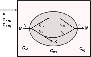
Interactions between cells and bioreactor. Schematic representation of major fluxes into cells in a bioreactor during a fed‐batch process. Substrates, represented by M_i, are consumed with specific rates r_i either associated with growth, with specific rate r_i,c, or independent of growth with specific rate r_i,nc. Part of the growth associated consumption of M_i is converted to products M_j with a specific rate r_j,c. A fraction of M_j is produced not correlated with growth with specific rate r_j,nc. Substrate M_i and product M_j are also added by feeding them with a volume rate F.

The rates of substrate consumption, r_i, and product formation, r_j, are both calculated from experimental data by rearranging Equation (1):

$$r_i=\left(-F.C_{F,Mi}+\frac{d(V_R.C_{Mi})}{dt}\right).\frac{1}{C_{XR}.V_R}$$ (4)

The derivative was computed by dividing the change of total quantity of metabolite M_i by the length of the respective period in a defined period.

For products, index j is used. In matrix notations, Equations (2) and (3) read

$$\left[\begin{array}{c}\hfill r_i\hfill \\ \hfill r_j\hfill \end{array}\right]=R=A.\mu +B=\left[\begin{array}{c}\hfill a_i\hfill \\ \hfill a_j\hfill \end{array}\right].\mu +\left[\begin{array}{c}\hfill b_i\hfill \\ \hfill b_j\hfill \end{array}\right]$$ (5)

where R, A and B are vectors with A and B constant within each metabolic phase.

As a practical consequence, the specific production rate of each metabolite can be expressed as a function of the growth rate by using joined linear sub‐models corresponding to distinct metabolic phases. The breakpoints between each sub‐model correspond to metabolic shifts.

Data Cleaning and Outlier Identification

As experimental data contain errors that may corrupt the conclusions, outliers must be identified. In particular, at low viable cell density during culture startup, computed specific production rates are inherently noisy and make interpretation of cell metabolism difficult. We thus identified outliers on the first days of production. For each day from day 0 to 2, data of all experiments was pooled since the conditions were identical until the feed addition started on day 3. Then principal components analysis (PCA) was performed on all the specific production rates of all metabolites for all experiments of this initial period to reduce the dimensionality of the data (Bersimis et al., 2005). The multidimensional distance from a sample point to its sample mean was then estimated using the T² Hoteling distance (Bersimis et al., 2005; Mason, 1997). Values that fall outside an upper control limit (UCL_T ²) are defined as outliers assuming the data follows a multidimensional normal distribution. The UCL on the T² distance is defined as:

$${UCL}_{T^2}=\frac{{(n-1)}^2}{n}{\beta }_{[1-\alpha ;\frac{p}{2};\frac{n-p-1}{2}]}$$ (6)

where

1. n = number of observations

2. P = number of variables

${\beta }_{[1-\alpha ;\frac{p}{2};\frac{n-p-1}{2}]}=(1-\mathrm{\alpha }\mathrm{th})$ quantile of a Beta $(\frac{p}{2};\frac{n-p-1}{2})$ distribution

This scheme is iterated until no more outliers are identified (Fig. 2).

Figure 2.

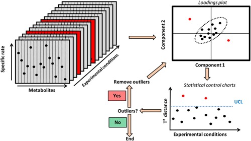
Schematic representation of the data cleaning process. A principal component analysis (PCA) is performed, for each day from day 0 to 2 separately, on a pool of the specific production rates of all metabolites. The T² Hotelling distance (Bersimis et al., 2005; Mason 1997) is then computed by assuming a multi‐normal distribution for the data. A simple statistical process control (SPC) (Bersimis et al., 2005; Mason 1997) is then used on these T² values to identify possible outliers. This scheme is repeated until no more outlier is identified. UCL: upper control limit. This methodology has been used on day 0, 1, and 2 of the cell cultivation since the experimental conditions are similar before the feeding starts on day 3.

It is important to conduct this data cleaning procedure during the first few days of the culture because the viable cell concentration during that period is low with correspondingly higher experimental error than in later cultivation phases. The coefficient of variation of the viable cell concentration method at these low cell concentrations was around 20% leading to very noisy rate calculations. On top of the outlier identification with PCA between day 0 and 2, two constraints were added for later data points:

1. All the data points with viability below 50%, that were usually only observed in later culture phases, were removed from the dataset as low cell viability can also lead to biased and incorrect estimation of the specific production rates of metabolites. This is due to metabolites released from cell death and to imprecision of the viable cell concentration measurements at this low cell viability.

2. Data points with depletion of metabolites during a measurement interval were also removed from the dataset as the computation of the specific production rate of that metabolite would be underestimated in these cases.

Identification of the Number of Metabolic Phases

To avoid over fitting with the segmented regression, the number of phases has to be determined. Based on the metabolic‐steady state paradigm, we assume that the vectors A and B (Equation (5)) are constant within a metabolic phase. We can estimate coefficients A for all metabolites for the whole cell culture process by taking the derivative of metabolic rates with respect to the specific growth rate, μ:

$$\frac{dR}{d\mu }=A$$ (7)

Vector A is assumed constant within each metabolic phase. As the derivative can amplify possible biological and analytical errors, the specific production rates were, preliminarily to deriving, smoothed as a function of the specific growth rate with the linear Locally Weighted Scatterplot Smoother (LOWESS) method (Cleveland, 1979) by using SAS software JMP 11 ©. The LOWESS method represents non‐parametric statistics that do not require any specific model. We used a “tricube” function (Cleveland, 1979) as a weight function and for each fitted value, a fraction of the data points of 0.5 was used for the computation. The weight function W is defined as:

$$W\left(x\right)=\{\begin{array}{cc}\hfill {(1-{\left|x\right|}^3)}^3\hfill & \hfill \mathrm{f}\mathrm{o}\mathrm{r}\left|x\right|<1\hfill \\ \hfill 0\hfill & \hfill \mathrm{o}\mathrm{t}\mathrm{h}\mathrm{e}\mathrm{r}\mathrm{w}\mathrm{i}\mathrm{s}\mathrm{e}\hfill \end{array}$$ (8)

The derivatives of the LOWESS function is then also computed with JMP 11 ©. The recursive partitioning (Gaudard et al., 2006) is then used on the smoothed derivatives defined in Equation (7): the data is successively partitioned according to a splitting value for a given factor. The splitting value is the one that maximize the −log(P‐value), also called logworth, of the chi‐square test measuring how different data is between the two partitions. The purpose of partitioning is to split all derivatives dR/dμ of each metabolite (Equation (7)), as a function of the specific growth rate and then to determine the number of breakpoints. On the dataset of all breakpoints for all metabolites, we apply a hierarchical clustering to identify similar set of breakpoint values (Mojena, 1977; Murtagh, 1983; Szekely and Rizzo, 2005) (Fig. 3). Each observation starts in its own cluster, and at each step the clustering process calculates the distance between each cluster, and combines the two clusters that are closest together (agglomerative procedure). The agglomerative procedure is Ward's method (Murtagh, 1983). The linkage distance is defined as the “cost” in between‐class sum of square to join the clusters. The final number of clusters selected is chosen as the first “knee” point in the linkage function, that is the peak in the second‐order derivative of the linkage distance function. The outcome is a first estimation of the breakpoint value of each metabolic phase and the total number of metabolic phases.

Figure 3.

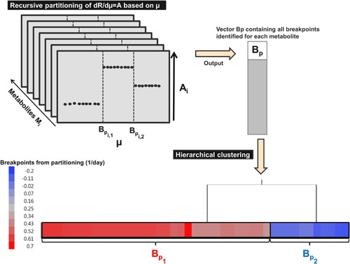
Identification of the number of metabolic phase breakpoints. Hierarchical clustering was performed on the vector containing the breakpoint growth rate values identified from recursive partitioning. Each observation/breakpoint starts in its own cluster, and at each step the clustering process calculates the distance between each other cluster, and combines the two clusters that are closest together (Agglomerative procedure) (Murtagh 1983). The agglomerative procedure uses the Ward's method to calculate the distance between each cluster. The objective was to identify the number of distinct metabolic phase breakpoints required to calibrate the segmented regression model (Fig. 3). Two groups of breakpoints were identified, which correspond to two metabolic phase breakpoints B_P1 and B_P2. B_P1 = 0.54 ± 0.06 day⁻¹; B_P2 = −0.08 ± 0.06 day⁻¹.

Segmented Linear Regression

Linear segments between all specific metabolic rates with the specific growth rate, μ, were identified using segmented linear regression analysis (McGee and Carleton, 1970; Ryan et al., 2007; Toms and Lesperance, 2003). It is a regression model composed of a sequence of joined linear sub‐models. If we define r_k as the observed specific production rate of metabolite M_k and μ as the growth rate, we have, for n ≥ 2 metabolic phases and n‐1 breakpoints B_{P s} such that $s\in \left\{\text{1,}\dots \text{,n‐1}\right\}$:

$$r_k\left(\mu \right)=a_{k,1}\cdot \mu +b_{k,1}+{\displaystyle {\displaystyle \sum }_{s=1}^{n‐1}}{a}_{k,s+1}\cdot (\mu -B_{P_j})\cdot u_s$$ (9)

$$u_s=\{\begin{array}{c}\hfill 1for\mu \le B_{P_s}\hfill \\ \hfill 0for\mu >B_{P_s}\hfill \end{array}1\le s\le n-1$$

b_i,1, a_i,1, a_i,j+1, and $B_{P_j}$ constant coefficients of metabolite M_i, for j∊{1,…,n‐1}. This expression allows the regression function to be continuous at the breakpoint (Ryan et al., 2007). Amino acid limitation in the medium can lead to its depletion that would impact mAb and protein synthesis (Gramer, 2014; Kilberg et al., 2009). As an extra constraint imposed to our model, as soon as an essential amino acid is depleted, the specific mAb productivity predicted by the model is set to zero. We consider tryptophan, histidine, isoleucine, methionine, threonine, phenylalanine, valine, tyrosine, leucine, lysine, glutamine, arginine, and cysteine as essential amino acids (Hu, 2012).

Parameter Estimation

For each metabolite, based on the number n of metabolic phases determined by the hierarchical clustering, n models were set up from zero to n‐1 breakpoints. For each model, the estimation of model parameters with the best fit was selected using a least‐square minimization (Wagner et al., 2002). To assess if the addition of a breakpoint makes the model prediction statistically superior to a model with a lower number of breakpoint, an F‐test was performed at 95% confidence level. To alleviate the selection of too close breakpoints, a criterion has been added to the model:

$$\left|B_{P1}-B_{P2}\right|>0.2da{y}^{-1}$$

A summary of the methodology is presented in Figure 4. All estimations were carried out using EXCEL (Microsoft) for primary data treatment and Matlab Release 2013a (The Mathworks, Natick, MA) for further calculations unless otherwise stated. MATLAB scripts are supplied as Supplementary Material to automatically carry out segmented linear regression using a supplied data set.

Figure 4.

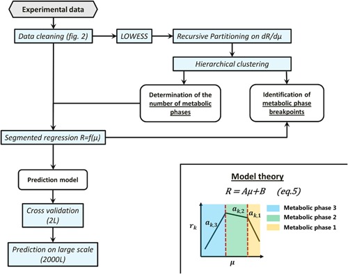
Developed methodology to identify and characterize metabolic phases. Experimental data are first cleaned using the methodology presented in Figure 2 and additionally by removing data with a viability below 50% or a depletion of metabolites during a measurement interval. The number of metabolic phases during the cell culture process are determined by differentiating the smoothed (LOWESS) reaction rates of all metabolites with respect to the growth rate (dR/dµ). Recursive partitioning is then applied on those derivatives to get a vector of possible metabolic phase breakpoints. Hierarchical clustering is then applied on this vector of possible breakpoints to define the number of final metabolic phases (clusters). Knowing the number of metabolic phases, the segmented regression can then be calibrated on the calibration dataset for each metabolite and validated on the cross validation dataset of the 2 L bioreactor and also of the 2000 L bioreactor.

Materials and Methods

Cell Line, Cell Cultivation, Sampling, and Rate Estimations

A CHO‐DG44 cell line was used. The cells were cultivated in a proprietary, chemically defined, serum‐free medium in 2 L stirred tank glass bioreactor (STR) with supply towers (C‐DCUII, Sartorius Stedim Biotech) controlled by a multi‐fermentation control system (MFCS, Sartorius Stedim Biotech). The reactors were equipped with a 3‐segment blade impeller (elephant ear impeller). The cultivation start volume was adapted to ensure an optimal cultivation end volume. The production bioreactors were seeded at similar target seeding density (TSD). The pH was controlled at a value of 7 with a dead band of 0.2. Dissolved oxygen concentration (pO2) was set to 40% air saturation. To control pO2, air, nitrogen, and oxygen were sparged into the culture using a cascade controller with a predefined mixture profile. The temperature was controlled at 36.8°C.

The culture was operated in fed‐batch mode for 14 days. During the feeding phase, the monoclonal antibody (mAb) is secreted into the medium. Samples were drawn daily to determine total and viable cell number, viability, off‐line pH, partial pressure of CO₂, pCO₂, osmolality, glucose‐lactate, amino acid, and mAb concentrations (stored at −80°C). Antifoam was added manually on demand every day to control the build‐up of foam. Seventy‐two hours after inoculation, continuous nutrient feeding with constant rate for a day was started with a predetermined rate using a proprietary, chemically defined concentrated feed. The feed rate was adjusted every day following a predefined strategy. In addition to that proprietary chemically defined concentrated feed addition, a glucose solution of 500 g/L was added as a bolus to the culture when the glucose concentration dropped below 6 g/L but only from day 6 onwards. In this way, glucose was not depleted at any time during the culture at the experimental conditions tested. Samples for the amino acid analysis were taken before the feed addition. The extracellular concentrations after feeding were computed based on the feed composition information. Specific growth rate, µ, was computed for each experimental condition separately as the slope of the linear trend line obtained by plotting ln(C_XR.V_R) against time (Chin et al., 2015; Clarke et al., 2011).

Experimental Condition

Various feed compositions of amino acid were tested in small scale bioreactors (2 L) for a total of 29 experimental conditions. We varied the concentration of three different amino acids (aa1, aa2, aa3) contained in our feed as described in the Supplementary Table SI.

The volume of feed added per bioreactor volume in the STR was the same in each condition. pH, temperature, stirrer speed, and all the bioreactor parameters were controlled at the same value. The TSD was also the same for all experiments. Three 2000 L production runs with the same experimental conditions were also performed, that is with identical feed addition profiles and chemically defined feed with a composition concerning the varied amino acids as specified in the supplementary Table S1. The set points for temperature, pH and pO2, as well as the target seeding density, medium formulation, nutrient feed formulation, feeding strategy, and culture duration were the same as at the 2 L bioreactor scale.

Analytical Methods

Cells were counted by using a VI‐CELL® XR (Beckman‐Coulter, Inc., Brea, CA) automated cell counting device that applied the trypan blue exclusion method. Glucose and lactate levels in the culture medium were determined using a NOVA 400 BioProfile automated analyzer (Nova Biomedical, Waltham, MA). A model 2020 freezing‐point osmometer (Advanced Instruments, Inc., Norwood, MA) was used for osmolality determination. Offline gas and pH measurements were performed with a BioProfile pHOx® blood gas analyzer (Nova Biomedical Corporation, Waltham, MA). Product titer analysis was performed with a ForteBio Octet model analyzer (ForteBio, Inc., Menlo Park, CA) or protein A high performance liquid chromatography (HPLC) with cell culture supernatant samples which were stored at −80°C prior to analysis. Amino acids were analyzed by reversed‐phase UPLC (Waters AccQ · Tagultra method) after ultra‐filtration using Amicon Ultra‐0.5 mL centrifugal filters (Merck Millipore, Billerica, MA). Statistical analysis were performed using SAS software JMP 11 ©. Matlab Release 2013a (The Mathworks, Natick, MA) was used to calibrate the segmented linear model.

Results and Discussion

The growth profile of all experimental conditions is depicted in Figure 5a. The growth behavior varies with the experimental conditions. For further analysis, we computed the specific production rates, r_i, of glucose, lactate, ammonia, all amino acids, and the mAb.

Figure 5.

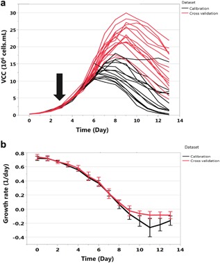
Experimental viable cell count and time course of specific growth rates. (a) Growth profiles of CHO‐DG44 for 29 experimental conditions (see supplementary Table SI) with various cell growth behaviors. The cells were cultivated in a 2 L bioreactor operated in fed‐batch mode for 14 days. Black arrow: Start of nutrient feeding with a predetermined rate. (b) Specific growth rate of the 29 experimental conditions after data cleaning (Fig. 2) for the calibration dataset and the cross validation dataset.

Data Cleaning and Determination of the Number of Metabolic Phases

We applied the outlier identification methodology based on the PCA on our dataset for days 0, 1, and 2 separately. From a total of 404 data points, 86 data points are from days 0, 1, and 2. From these 47 outliers were identified by using PCA and removed from the dataset. Based on the two extra constraints added to our data cleaning procedure from day 3 to 14, data points with depletion of metabolites and/or with viability lower than 50% throughout the cell culture production were also removed from the dataset resulting in a total of 215 remaining data points. This cleaned dataset was partitioned into two datasets based on the growth rate profiles of each experimental condition: 115 data points (calibration dataset) with a wide range of experimental conditions as specified in the Supplementary Table SI and 100 data points (cross validation dataset) with similar experimental conditions. The cross validation dataset contains experimental conditions within the design space of the calibration dataset. From the calibration dataset, two distinct clusters, which correspond to the breakpoints, were identified based on recursive partitioning and hierarchical clustering as described above (Fig. 3): one (B_p1) at a growth rate of 0.54 ± 0.06 day⁻¹ and a second one (B_p2) at −0.08 ± 0.06 day⁻¹. The first breakpoint was identified for all metabolites. The second breakpoint was only identified for proline, valine, leucine, methionine, tyrosine, threonine, cysteine, asparagine, lysine, glutamate, lactate, and mAb. Hence, to avoid over fitting during the calibration of the segmented linear regression, the maximum number of breakpoints to identify was set to two.

Calibration of the Prediction Model Using the Segmented Regression Model

Segmented regression was applied on the cleaned calibration dataset, containing specific growth rates and not smoothed specific production rates of metabolites and mAb (Fig. 6a). The identification of the metabolic phase breakpoints and the calibration of models were performed separately for each metabolite. Estimated model parameters are listed in Table I. Twelve metabolites, that is ammonium, glycine, alanine, methionine, serine, asparagine, glutamine, arginine, aspartate, glutamate, glucose, and lactate, are impacted by metabolic phases. These metabolites are linked to glucose/glutamine metabolism and cell proliferation which confirms results of Rehberg et al. (2014). Most models for these metabolites include only one breakpoint, that is only two metabolic phases were identified. Only glutamate, methionine, and lactate have a specific production rate profile divided into three metabolic phases. Based on an F‐test, twelve metabolites are better fitted with a simple linear regression model and not impacted by metabolic phases: proline, isoleucine, leucine, lysine, valine, phenylalanine, cysteine, tyrosine, tryptophan, threonine, histidine, and mAb (Fig. 6a).

Figure 6.

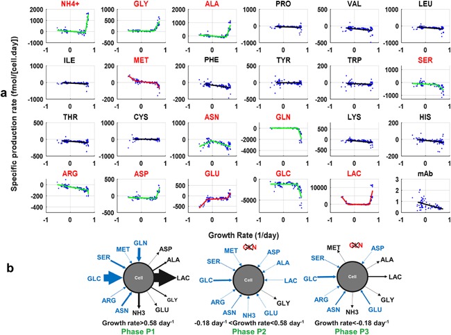
Segmented regression of specific rates as a function of the growth rate. To identify metabolic phases, segmented regression was used (Fig. 4). Data of the 2 L bioreactor calibration dataset were used. Three models were set up for each metabolite, from zero up to two breakpoints. To assess whether the addition of a breakpoint makes the model prediction statistically superior to a model with a lower number of breakpoints, an F‐test was performed with 95% confidence level. (a) Segmented regression models are presented. Red names correspond to metabolites that are impacted by metabolic phases, that is which show better prediction with one to two breakpoints. When the segmented regression model is characterized by a red line, three metabolic phases were identified. Identification of two metabolic phases are characterized by a green line. (b) The 12 metabolites that were significantly impacted by metabolic phases are presented for each metabolic phase: P1, P2, and P3. Blue arrow: net uptake; Dark arrow: net secretion. The widths of the arrows are proportional to the average specific production rate values for the defined metabolic phase.

Table I.

Segmented model coefficients. For each metabolites and for each metabolic phase, the value of coefficient a and b from equation (5) is presented

	a (10−09 mmol/cell)			b (10−09 mmol/cell.day)
	P1	P2	P3	P1	P2	P3
NH4+	12.45 (9.90)	−0.16 (−0.18)		−7.81 (−6.10)	0.04 (0.04)
Gly	2.04 (2.12)	−0.002 (0.08)		−1.07 (−1.15)	0.02 (0.02)
Ala	5.15 (4.78)	−0.11 (0.02)		−3.03 (−2.84)	0.02 (−0.02)
Pro	−0.05 (−0.10)			−0.06 (−0.04)
Val	−0.06 (−0.13)			−0.09 (−0.06)
Leu	−0.09 (−0.14)			−0.12 (−0.08)
Ile	−0.07 (−0.03)			−0.06 (−0.04)
Met	−0.46 (−0.57)	−0.03 (−0.006)	−0.24 (N/A)	0.28 (0.36)	0.01 (0.0044)	−0.04 (N/A)
Phe	−0.04 (−0.05)			−0.03 (−0.02)
Tyr	−0.00009 (−0.05)			−0.06 (−0.03)
Trp	−0.009 (−0.012)			−0.02 (−0.01)
Ser	−1.47 (−1.87)	−0.08 (−0.17)		0.48 (0.14)	−0.18 (−0.14)
Thr	−0.04 (−0.09)			−0.07 (−0.05)
Cys	0.01 (−0.06)			−0.07 (−0.05)
Asn	−0.44 (−0.49)		0.78 (N/A)	−0.25 (−0.17)		−0.11 (N/A)
Gln	−12.39 (−12.17)	−0.03 (−0.06)		7.42 (7.38)	0.007 (0.007)
Lys	−0.10 (−0.20)			−0.10 (−0.06)
His	−0.03 (−0.05)			−0.01 (−0.009)
Arg	−3.14 (−0.72)	−0.08 (−0.09)		2.19 (0.38)	−0.03 (−0.03)
Asp	1.97 (1.49)	−0.02 (−0.02)		−1.25 (−0.95)	−0.05 (−0.05)
Glu	1.84 (1.31)	0.07 (0.05)	1.20 (N/A)	−1.19 (−0.85)	−0.09 (−0.09)	0.18 (N/A)
Glc	−18.34 (−18.58)	−0.04 (−0.21)		9.61 (10.00)	−0.98 (−0.88)
Lac	63.41 (56.79)	−0.05 (0.15)	−17.66 (N/A)	−39.42 (−35.51)	0.03 (−0.06)	−4.86 (N/A)
mAb	−0.0006 (−0.0002)			0.0007 (0.006)

The coefficients were also identified with the cross validation dataset and presented in the brackets. Red names correspond to metabolites that are impacted by the three metabolic phases. Bold names are metabolites that are impacted by two metabolic phases. Glc − glucose; Lac − lactate, mAb − monoclonal antibody.

Suitability of the Segmented Model to Identify Metabolic Phases

Breakpoints were identified for 12 metabolites. For the 12 metabolites that have significant breakpoints, the breakpoints B_p1 and/or B_p2 identified share similar values with a relative precision of breakpoint identification close to 5% for both breakpoints which supports the suitability of the method. The relative precision is defined here as the standard deviation divided by the range of the possible growth rate values. The first breakpoint between phases P1 and P2 was reached when the initially high specific growth rate, μ, decreased below a value of 0.58 ± 0.09 day⁻¹, the second one between phases P2 and P3 when μ fell below −0.18 ± 0.09 day⁻¹ (Fig. 6b). The segmented linear regression identified breakpoint B_p1 for only 11 metabolites and breakpoint B_p2 for 4 metabolites (Table I) which is less than those identified with the combination of recursive partitioning and hierarchical clustering. This may be explained by the sensitivity of the second method to outliers: the LOWESS regression may create additional trends that only exist due to possible outliers and the derivative computation can amplify the noise. Moreover, no F‐test is performed with the combination of recursive partitioning and hierarchical clustering which could possibly identify non‐significant metabolites. Nevertheless, breakpoints identified by both methods are similar which proves the reliability of the segmented linear regression to identify metabolic phases. As a conclusion from our work, the application of segmented regression is sufficient to identify relevant breakpoints and parameter. Therefore, hierarchical clustering is not necessary which simplifies the overall procedure.

The first metabolic phase P1, defined by a high growth rate, is characterized by a high production of ammonium, glycine, alanine, lactate, glutamate, and aspartate and a high consumption of methionine, asparagine, arginine, serine, glucose, and glutamine. This is a common metabolic profile observed in literature with suspension CHO cells also called overflow metabolism (Niu, et al., 2013; Wahrheit, 2015) or exponential phase (Amribt et al., 2013; Dorka et al., 2009; Meshram et al., 2013). All the other amino acids are also consumed during this first metabolic phase but the rates are lower than those of the 12 metabolites impacted by metabolic phases. During phase P1, lactate is a byproduct of the glycolysis and high excretion of alanine is due to the conversion of pyruvate to alanine via the alanine aminotransferase (ALAT) serving as a nitrogen sink. Glycine synthesis is a result of high serine uptake which is generally observed for mammalian cells and can be linked to nucleotide synthesis and to cell proliferation (Narkewicz et al., 1996). Glutamine is taken up as a carbon source for the tricarboxylic acid cycle (TCA) cycle and hydrolyzed into glutamate and ammonium. Asparagine is partly converted into aspartate which can then be converted into oxaloacetate. In the second metabolic phase P2 (Fig. 6b), the growth rate further decreased and some metabolites, that is ammonium, alanine, lactate, glutamate, and aspartate, started being consumed. This metabolic phase is usually called balanced metabolism (Wahrheit et al., 2014b; Wahrheit, 2015) or transition phase (Naderi et al., 2011; Provost et al., 2006; Zamorano et al., 2013). Overall, the rates of all metabolites were lower than in phase P1. Alanine and lactate, accumulated during the phase P1, were converted back to pyruvate, which is a major characteristic of CHO cell metabolism. The last metabolic phase P3 (Fig. 6b) is characterized by an accumulation of methionine, an increase of the consumption of glutamate and asparagine, and an overproduction of lactate. For the other eight metabolites that were impacted by the first metabolic shift, no break of slope could be observed between phases P2 and P3. The growth rate is negative for that metabolic phase, also called in the literature the maintenance phase (Wahrheit, 2015; Yu et al., 2011) or death phase (Provost et al., 2006; Zamorano et al., 2013).

Usually, different growth behaviors can be observed during process production, making it quite difficult to compare their metabolic characteristics by only using time. Using the growth rate rather than time allows better identification of metabolic phases and better comparison of their characteristics between various experimental conditions particularly in fed‐batch cultivation.

Validation of the Model at Small Scale (2 L)

Metabolic profiles of the cross validation dataset were predicted (Fig. 7) from the experimental growth rate of the cross validation dataset and parameters of segmented regression model identified using the calibration dataset (Table I). Since the growth rates were overall similar in the cross validation dataset, the data can be presented as a function of time. The model prediction closely followed the experimental trends throughout the cell culture process. The only discrepancy occurred in the late stages, on day 13, for 18 metabolites. For four metabolites, that is tyrosine, tryptophan, cysteine, and glucose, the prediction is also out of range for day 12.

Figure 7.

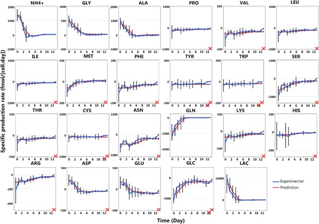
Cross validation of the segmented regression models for each metabolite in 2 L bioreactor runs. The specific production rates of all metabolites for the validation dataset are presented as a function of time (day) as the specific growth rate profiles were similar (Fig. 5). The error bars correspond to 3 standard deviations. The prediction (red line) is based on the segmented regression of the calibration dataset (Fig. 6) and used the experimental specific growth rate profile (Fig. 5b) to estimate specific production rates. The prediction variability is due to the growth rate value variability and the error bars presented for the prediction correspond also to the three standard deviation. When the prediction was out of the 3 standard deviations range, the corresponding day is crossed in red.

Prediction of the Specific Production Rate in Large Scale (2000 L)

To estimate the transferability of the segmented regression model to a larger scale cultivation, specific production rates of metabolites of each 2000 L experiment were predicted (Fig. 8) by the model estimated on the 2 L bioreactor calibration set (Table I). As the growth rates were similar for the triplicate experimental conditions, the data could be presented together as a function of time. The prediction model is able to track the experimental trends of almost all metabolites over the entire culture period. Overall 88% of the predictions fall into a 3 standard deviations interval. Two amino acids, named aa1 and aa2, were depleted throughout the cell culture process but the model was able to predict their concentrations (Fig. 9b).

Figure 8.

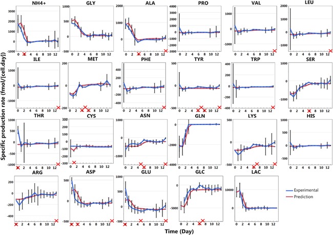
Validation of the segmented regression models for each metabolite at 2000 L bioreactor scale. The specific production rates of each metabolites for three 2000 L bioreactors runs with the same experimental condition are presented as a function of time (day) as the specific growth rate profiles are similar. The error bars correspond to 3 standard deviations. The prediction model (red line) is based on the segmented regression of the calibration dataset (Fig. 6) and is based on the experimental specific growth rate profile (Fig. 5b). The prediction variability is due to the growth rate value variability and the error bars presented for the prediction correspond also to the three standard deviation. When the prediction was out of the 3 standard deviations range, the corresponding day is crossed in red.

Figure 9.

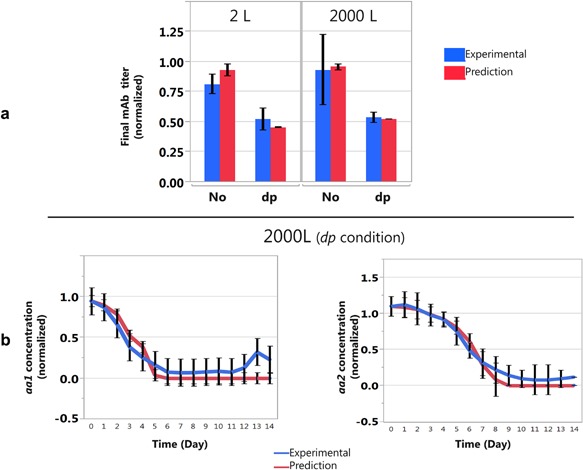
Prediction of the final mAb titer and of aa1 and aa2 concentrations. (a) Experimental and predicted final mAb titers for the calibration dataset (2 L) and for large scale bioreactor runs (2000 L). The mAb titers were normalized to the maximum titer reached. The prediction is based on the segmented regression model of the specific productivity. The calibration dataset (2 L) and the large scale bioreactor runs (2000 L) are divided into 2 subsets: one without depletion of any metabolite during the cell culture process (No), and the other with depletions of aa1 and aa2, two amino acids, during the cell culture process (dp). The error bars correspond to 3 standard deviations for both prediction and experimental data. (b) Prediction of aa1 and aa2 concentrations before feeding during the whole cell culture process in triplicate experiments in 2000 L bioreactors (dp). The concentrations were normalized to the initial concentrations.

Accuracy of the Segmented Model for Prediction of Metabolite Profiles (2 and 2000 L)

Cross validation of the segmented models showed good results for all metabolites. The ability to predict the experimental metabolite profiles in large scale experiments reinforces the validity of the model and justifies the initial assumption of linear correlation of specific rates of metabolites with the specific growth rate. The accuracy of our model with two to a maximum of six parameters to estimate for each metabolite is remarkable. For 12 metabolites, even if a simple linear model was used, the model has provided accurate results. Moreover, adding more parameters to the model may lead to over fitting. From this point of view, the model can be used for accurate prediction of the specific production rates of metabolites and so, of the metabolite concentrations, requiring only the experimental specific growth rate of the prevailing experiment. The established model would also allow online estimation of metabolic rates on the bases of online measured biomass parameters, for example viable cell count. It could therefore potentially also be applied for on line optimization of feeding profiles.

Accuracy of the Segmented Model for Prediction of Final mAb Titers (2 and 2000 L)

The model was used to predict the final mAb titer. Results of prediction model are presented in Figure 9a. The final mAb titer prediction in 2 L is accurate and within the range of  ±3 standard deviations even for conditions with a depletion of metabolites throughout the cell culture process. Similarly to the small scale, the 2000 L triplicate experimental conditions previously used to compare the metabolite prediction profiles were depleted in some metabolites, that is aa1 and aa2, during the cell cultivation. Hence, the prediction of the final mAb titer in 2000 L is also compared to other duplicates experimental conditions in 2000 L bioreactors runs without metabolites limitations throughout the cell culture process. The final mAb titer prediction is accurate and within the ±3 standards deviations even with metabolite limitations throughout the cell culture process (Fig. 9a). Our model is able to predict mAb titer decrease due to essential amino acid depletion.

Prediction Outside Calibration Experimental Conditions

The segmented regression methodology was used to identified coefficients a and b from equation  10 with the cross validation dataset. The objective was to compare both coefficients identified with the cross validation dataset and with the calibration dataset. Results are presented in Table I in the brackets and in supplementary material (Fig. S1). As expected, the breakpoints B_p2 was not identified with the cross validation dataset as the growth rates minimum values were higher than B_p2. For coefficients a and b within metabolic phase P1 and P2, coefficients are similar which prove the predictability and applicability of the methodology. As the cross validation dataset only contained four different experimental conditions, we can conclude from this work that the presented method does not require a wide range of different experimental conditions in order to set up a robust and predictive model. The question of the minimum of data points and experiments needed is difficult to answer, since it depends on the quality of the measured data.

Conclusion

In summary, we propose an accurate predictive model of external metabolite rates which requires few parameters to estimate and seems very robust. The final titer can also be predicted even if the cells are starved in some metabolites. It should also be highlighted that an entire and complex metabolic network is not needed in order to achieve the macroscopic modeling which makes it simpler and, possibly, easily adaptable to other cell clones and cell lines. We also presented a systematic methodology to identify metabolic phases that allows comparing various experimental conditions with different growth behavior. It provides an excellent basis for later metabolic flux analysis and for later dynamic mechanistic modeling. We showed that the metabolites that are more impacted by metabolic shift are those linked to glucose/glutamine metabolism and cell proliferation.

Supporting information

Additional supporting information may be found in the online version of this article at the publisher's web‐site.

Figure S1. Comparison of segmented model coefficients. For each metabolite and for each metabolic phase, the values of coefficients a and b from Equation (5) were identified with the calibration dataset and the cross validation dataset.

Table S1. Experimental conditions. The concentration of three different amino acids (aa1, aa2, aa3) contained in the feed that were varied. They are presented as percentage of the maximum concentration tested.

References

- Altamirano C, Illanes A, Becerra S, Cairó JJ, Gòdia F. 2006. Considerations on the lactate consumption by CHO cells in the presence of galactose. J Biotechnol 125(4):547–556. [DOI] [PubMed] [Google Scholar]
- Altamirano C, Illanes A, Casablancas A, Gámez X, Cairó JJ, Gòdia C. 2001. Analysis of CHO cells metabolic redistribution in a glutamate‐Based defined medium in continuous culture. Biotechnol Prog 17(6):1032–1041. [DOI] [PubMed] [Google Scholar]
- Amribt Z, Niu H, Bogaerts P. 2013. Macroscopic modelling of overflow metabolism and model based optimization of hybridoma cell fed‐batch cultures. Biochem Eng J 70(0):196–209. [Google Scholar]
- Ashyraliyev M, Fomekong‐Nanfack Y, Kaandorp JA, Blom JG. 2009. Systems biology: Parameter estimation for biochemical models. FEBS J 276(4):886–902. [DOI] [PubMed] [Google Scholar]
- Ben Yahia B, Malphettes L, Heinzle E. 2015. Macroscopic modeling of mammalian cell growth and metabolism. Appl Microbiol Biotechnol 99(17):7009–7024. [DOI] [PMC free article] [PubMed] [Google Scholar]
- Bersimis S, Panaretos J, Psarakis S, Volkswirtschaftliche Fakultät L‐M‐UM. 2005. Multivariate statistical process control charts and the problem of interpretation: a short overview and some applications in industry. Transport Res B‐Meth 81(P1):78–102. [Google Scholar]
- Borchers S, Freund S, Rath A, Streif S, Reichl U, Findeisen R. 2013. Identification of growth phases and influencing factors in cultivations with AGE1.HN cells using set‐Based methods. PLoS ONE 8(8):e68124. [DOI] [PMC free article] [PubMed] [Google Scholar]
- Chin CL, Chin HK, Chin CS, Lai ET, Ng SK. 2015. Engineering selection stringency on expression vector for the production of recombinant human alpha1‐antitrypsin using Chinese Hamster ovary cells. BMC Biotechnol 15:44. [DOI] [PMC free article] [PubMed] [Google Scholar]
- Clarke C, Doolan P, Barron N, Meleady P, O'Sullivan F, Gammell P, Melville M, Leonard M, Clynes M. 2011. Predicting cell‐specific productivity from CHO gene expression. J Biotechnol 151(2):159–165. [DOI] [PubMed] [Google Scholar]
- Cleveland WS. 1979. Robust locally weighted regression and smoothing scatterplots. J Am Stat Assoc 74(368):829–836. [Google Scholar]
- Dean J, Reddy P. 2013. Metabolic analysis of antibody producing CHO cells in fed‐batch production. Biotechnol Bioeng 110(6):1735–1747. [DOI] [PubMed] [Google Scholar]
- Deshpande R, Yang TH, Heinzle E. 2009. Towards a metabolic and isotopic steady state in CHO batch cultures for reliable isotope‐based metabolic profiling. Biotechnol J 4(2):247–263. [DOI] [PubMed] [Google Scholar]
- Dorka P, Fischer C, Budman H, Scharer J. 2009. Metabolic flux‐based modeling of mAb production during batch and fed‐batch operations. Bioprocess Biosyst Eng 32(2):183–196. [DOI] [PubMed] [Google Scholar]
- Fan Y, Jimenez Del Val I, Müller C, Lund AM, Sen JW, Rasmussen SK, Kontoravdi C, Baycin‐Hizal D, Betenbaugh MJ, Weilguny D, and others. 2015. A multi‐pronged investigation into the effect of glucose starvation and culture duration on fed‐batch CHO cell culture. Biotechnol Bioeng 112(10):2172–2184. [DOI] [PubMed] [Google Scholar]
- Gaudard M, Ramsey P, Stephens M. 2006. Interactive data mining and design of experiments: The JMP partition and custom design platforms. North Haven Group, LLC: CaryNorth Carolina. [Google Scholar]
- Gramer MJ. 2014. Product quality considerations for mammalian cell culture process development and manufacturing. Adv Biochem Eng/Biotechnol 139:123–166. [DOI] [PubMed] [Google Scholar]
- Hu W‐S. 2012. Cell culture bioprocess engineering. 1st edn p 162–166. ISBN: 978‐0‐9856626‐0‐8. [Google Scholar]
- Jungers RM, Zamorano F, Blondel VD, Wouwer AV, Bastin G. 2011. Fast computation of minimal elementary decompositions of metabolic flux vectors. Automatica 47(6):1255–1259. [Google Scholar]
- Kilberg MS, Shan J, Su N. 2009. ATF4‐dependent transcription mediates signaling of amino acid limitation. Trends Endocrinol Metab 20(9):436–443. [DOI] [PMC free article] [PubMed] [Google Scholar]
- Luedeking R, Piret EL. 1959. A kinetic study of the lactic acid fermentation. Batch process at controlled pH. J Biochem Microbiol Technol Eng 1(4):393–412. [DOI] [PubMed] [Google Scholar]
- Mason RL. 1997. A practical approach for interpreting multivariate T2 control chart signals. J Qual Technol 29(4):396–406. [Google Scholar]
- McGee VE, Carleton WT. 1970. Piecewise regression. J Am Stat Assoc 65(331):1109–1124. [Google Scholar]
- Meshram M, Naderi S, McConkey B, Ingalls B, Scharer J, Budman H. 2013. Modeling the coupled extracellular and intracellular environments in mammalian cell culture. Metab Eng 19(0):57–68. [DOI] [PubMed] [Google Scholar]
- Mojena R. 1977. Hierarchical grouping methods and stopping rules: An evaluation. The Comput J 20(4):359–363. [Google Scholar]
- Muggeo VM. 2003. Estimating regression models with unknown break‐points. Stat Med 22(19):3055–3071. [DOI] [PubMed] [Google Scholar]
- Mulukutla BC, Yongky A, Grimm S, Daoutidis P, Hu WS. 2015. Multiplicity of steady states in glycolysis and shift of metabolic state in cultured mammalian cells. PLoS ONE 10(3):e0121561. [DOI] [PMC free article] [PubMed] [Google Scholar]
- Murtagh F. 1983. A survey of recent advances in hierarchical clustering algorithms. The Computer Journal 26(4):354–359. [Google Scholar]
- Naderi S, Meshram M, Wei C, McConkey B, Ingalls B, Budman H, Scharer J. 2011. Development of a mathematical model for evaluating the dynamics of normal and apoptotic Chinese hamster ovary cells. Biotechnol Prog 27(5):1197–1205. [DOI] [PubMed] [Google Scholar]
- Narkewicz MR, Sauls SD, Tjoa SS, Teng C, Fennessey PV. 1996. Evidence for intracellular partitioning of serine and glycine metabolism in Chinese hamster ovary cells. Biochem J 313(Pt3):991–996. [DOI] [PMC free article] [PubMed] [Google Scholar]
- Niklas J, Heinzle E. 2012. Metabolic flux analysis in systems biology of Mammalian cells. Adv Biochem Eng/Biotechnol 127:109–132. [DOI] [PubMed] [Google Scholar]
- Niklas J, Schräder E, Sandig V, Noll T, Heinzle E. 2011. Quantitative characterization of metabolism and metabolic shifts during growth of the new human cell line AGE1.HN using time resolved metabolic flux analysis. Bioprocess Biosyst Eng 34(5):533–545. [DOI] [PMC free article] [PubMed] [Google Scholar]
- Niu H, Amribt Z, Fickers P, Tan W, Bogaerts P. 2013. Metabolic pathway analysis and reduction for mammalian cell cultures—Towards macroscopic modeling. Chem Eng Sci 102(0):461–473. [Google Scholar]
- Nolan RP, Lee K. 2011. Dynamic model of CHO cell metabolism. Metab Eng 13(1):108–124. [DOI] [PubMed] [Google Scholar]
- Pirt SJ. 1965. The maintenance energy of bacteria in growing cultures. Proc R Soc Lond B Biol Sci 163(991):224–231. [DOI] [PubMed] [Google Scholar]
- Pirt SJ. 1982. Maintenance energy: A general model for energy‐limited and energy‐sufficient growth. Arch Microbiol 133(4):300–302. [DOI] [PubMed] [Google Scholar]
- Provost A, Bastin G. 2004. Dynamic metabolic modelling under the balanced growth condition. J Process Control 14(7):717–728. [Google Scholar]
- Provost A, Bastin G, Agathos SN, Schneider YJ. 2006. Metabolic design of macroscopic bioreaction models: Application to Chinese hamster ovary cells. Bioprocess Biosyst Eng 29(5–6):349–366. [DOI] [PMC free article] [PubMed] [Google Scholar]
- Rehberg M, Rath A, Ritter JB, Genzel Y, Reichl U. 2014. Changes in intracellular metabolite pools during growth of adherent MDCK cells in two different media. Appl Microbiol Biotechnol 98(1):385–397. [DOI] [PubMed] [Google Scholar]
- Ryan SE, Porth LS, Rocky Mountain Research S. 2007. A tutorial on the piecewise regression approach applied to bedload transport data. Fort Collins, CO: U.S. Dept. of Agriculture, Forest Service, Rocky Mountain Research Station. ii, 41 p.
- Sidoli FR, Mantalaris A, Asprey SP. 2004. Modelling of mammalian cells and cell culture processes. Cytotechnology 44(1–2):27–46. [DOI] [PMC free article] [PubMed] [Google Scholar]
- Simon L, Karim MN, Schreiweis A. 1998. Prediction and classification of different phases in a fermentation using neural networks. Biotechnol Tech 12(4):301–304. [Google Scholar]
- Szekely GJ, Rizzo ML. 2005. Hierarchical clustering via joint between‐Within distances: Extending ward's minimum variance method. J Classif 22(2):151–183. [Google Scholar]
- Tescione L, Lambropoulos J, Paranandi MR, Makagiansar H, Ryll T. 2015. Application of bioreactor design principles and multivariate analysis for development of cell culture scale down models. Biotechnol Bioeng 112(1):84–97. [DOI] [PubMed] [Google Scholar]
- Toms JD, Lesperance ML. 2003. Piecewise regression: A tool for identifying ecological thresholds. Ecology 84(8):2034–2041. [Google Scholar]
- Tsang VL, Wang AX, Yusuf‐Makagiansar H, Ryll T. 2014. Development of a scale down cell culture model using multivariate analysis as a qualification tool. Biotechnol Prog 30(1):152–160. [DOI] [PubMed] [Google Scholar]
- Wagner AK, Soumerai SB, Zhang F, Ross‐Degnan D. 2002. Segmented regression analysis of interrupted time series studies in medication use research. J Clin Pharm Ther 27(4):299–309. [DOI] [PubMed] [Google Scholar]
- Wahrheit J. 2015. Metabolic dynamics and compartmentation in the central metabolism of Chinese hamster ovary cells. Saarländische Universitäts‐ und Landesbibliothek: Saarbrücken. [Google Scholar]
- Wahrheit J, Nicolae A, Heinzle E. 2014a. Dynamics of growth and metabolism controlled by glutamine availability in Chinese hamster ovary cells. Appl Microbiol Biotechnol 98(4):1771–1783. [DOI] [PubMed] [Google Scholar]
- Wahrheit J, Niklas J, Heinzle E. 2014b. Metabolic control at the cytosol‐mitochondria interface in different growth phases of CHO cells. Metab Eng 23(0):9–21. [DOI] [PubMed] [Google Scholar]
- Yu M, Hu Z, Pacis E, Vijayasankaran N, Shen A, Li F. 2011. Understanding the intracellular effect of enhanced nutrient feeding toward high titer antibody production process. Biotechnol Bioeng 108(5):1078–1088. [DOI] [PubMed] [Google Scholar]
- Zamorano F, Vande Wouwer A, Jungers RM, Bastin G. 2013. Dynamic metabolic models of CHO cell cultures through minimal sets of elementary flux modes. J Biotechnol 164(3):409–422. [DOI] [PubMed] [Google Scholar]
Associated Data
This section collects any data citations, data availability statements, or supplementary materials included in this article.
Supplementary Materials