

Abstract
The six elastic constants (and six elastic compliances) of rutile were determined in the kilocycle per second frequency range by a resonance method. The standard deviations range from 0.2 percent for s11 to 4.3 percent for s13.
1. Introduction
The electrical properties of rutile make it a promising material for solid state electronic devices and a large literature on such properties exists and has been surveyed [1, 2, 3].1 Comparatively little information on the mechanical properties of rutile was available until recently. The linear compressibilities had been measured by Bridgman [4], and a set of elastic constants was calculated from spectroscopic data by Dayal and Appalanarasimham [5]. No further work on elastic properties was apparently done until the recent independent and nearly simultaneous measurements of three groups. Vick, Hollander, and Brown [6], determined four of the six elastic constants of rutile directly from pulse velocity measurements and calculated the other two by combining Bridgman’s linear compressibilities with their own data. Verma [7] published a set of the elastic constants calculated from his pulse velocity measurements. The present writers reported [8] a set of values determined by least squares fitting of the theoretical equations for the orientation dependence for elastic moduli to a set of experimental values determined on 10 single-crystal rutile rods by resonance in the audiofrequency range. Appreciable discrepancies existed for some of the constants, especially between those of Verma and those of the other investigators. Vick and Hollander [9] checked their measurements and published a refined set of values which are little different from their first set. The most serious discrepancies were removed when it was discovered that the direction which Verma took to be [100] was in fact [110]. It is an interesting property of the 4/mmm crystalographic point group, to which rutile belongs, that the x axis may be taken as either [100] or [110] and a self consistent matrix of elastic constants results which has the same form (but three of the six constants will have different numerical values). There is thus no internal inconsistency in Verma’s work but his results should be expressed in terms of [100] as the x axis to agree with the usual convention and to permit direct comparison with other values. This calculation has been done by Birch [10] and the resulting values agree fairly well with the results of other in vestigators but not as well as would be expected from the accuracy of methods of measurement which were used. The present writers wished to refine their data; their initial results were based upon measurements on 10 rods whose rod axes were all near the [001] axis. A comparatively large uncertainty in c11 and c66 resulted. This situation was improved when six additional rods were eventually obtained and the present results agree well with the values calculated by Birch in the sense that there is now no statistically significant difference for any of the cij. The standard deviations are, however, appreciably larger than those obtained by the authors on corundum [11] using the same resonance method. The most important source of this variability is believed to be caused by the presence of a profusion of small angle boundaries whose existence is shown by hack-reflection Laue patterns.
The present paper gives the method of applying the resonance technique to tetragonal crystals because it apparently has not been previously described for this crystal system. The general method has been described previously and reference [11] may be consulted for general background.
2. Description of Specimens
All specimens were synthetic “single crystals” grown by the Verneuil flame-fusion technique using an oxygen-hvdrogen flame. Such specimens in the as grown state characteristically contain two types of defect: (1) they are oxygen deficient and (2) they have many small angle boundaries (as much as 2° misorientation across a single boundary). The first type of defect is easily removed by heating in oxygen at temperatures around 1,000 °C. Parenthetically we note that the difficult problems of obtaining exact stoichiometry and of measuring small deviations from stoichiometry do not concern us here. The elastic constants do undoubtedly depend to some extent on the degree of reduction but the effect is very small as noted by Vick and Hollander [9]. We have not carried out a systematic study of the effect of reduction on all of the cij but observations of the very small changes produced in several heavily reduced (jet black) rods indicate that the effect which the possible small remaining oxygen deficiency in our nominally stoichiometric rods may have on the cij at room temperature is too small to be of any concern. Heavy reduction did show a measurable effect on the temperature dependence of Young’s modulus at high temperature [12] but this is outside the scope of our present considerations. Our specimens were heated for about 24 hr in flowing O2 at about 800 °C and we consider them to be effectively stoichiometric.
The second type of defect appears in all rutile single crystals examined by the authors and no method of removing it is known. Back-reflection Laue patterns were taken at random on many specimens; perhaps one fourth of the patterns show double spots indicating a change of orientation of 1 or 2 deg. If this were a systematic, progressive change of orientation along a rod, one end would differ greatly in orientation from the other and the crystals would be useless for our work. Fortunately, as table 1 shows, this is not so. Laue patterns were taken at the center and at both ends of each rod. Duplicate patterns were taken on specimens 21 and 22 to indicate the precision of the method. The resulting standard deviations were 0.12° for θ and 0.16° for ϕ where θ and ϕ are the usual spherical polar angles. The colatitude, θ, is the angle between the rod axis and [001]; the angle ϕ is the angle between [100] and the projection of the rod axis on the (001) plane. The orientation apparently shifts back and forth in a random manner from one small angle boundary to another. The average values of θ and ϕ were used for each rod in the calculations. It is hoped that better temperature, atmosphere, and powder feed control during crystal growth would reduce the number of the boundaries and this is being attempted at the National Bureau of Standards and elsewhere.
Table 1.
Properties of “single crystal” rutile specimens
| Specimen number | Mass | Length | End
|
Center
|
Other end
|
|||
|---|---|---|---|---|---|---|---|---|
| θ | ϕ | θ | ϕ | θ | ϕ | |||
|
All angles in degrees | ||||||||
|
Linde rods | ||||||||
| g | cm | |||||||
| 21 | 2.6317 | 13.236 | 2.6 2.2 |
} 12.7 | 2.1 | 1.8 1.5 |
||
| 22 | 2.2113 | 13.178 | 12.5 12.5 |
} 38.9 | 10.2 | 8.0 8.1 |
||
| 23 | 2.8205 | 12.168 | 14.0 | 7.3 | 16.1 | 7.0 | 14.8 | 6.3 |
| 24 | 2.3654 | 11.714 | 43.3 | 34.1 | 45.6 | 37.9 | 44.7 | 33.6 |
| 25 | 2.3770 | 11.178 | 11.2 | 37.9 | 11.4 | 29.0 | 11.9 | 36.3 |
| 26 | 1.2718 | 7.534 | 8.0 | 26.6 | 7.8 | 22.8 | 8.4 | 26.1 |
| 27 | 1.2769 | 6.986 | 14.6 | 18.8 | 14.2 | 19.0 | 15.0 | 20.9 |
| 28 | 1.2561 | 6.080 | 39.0 | 40.0 | 42.4 | 40.0 | 43.0 | 45.0 |
| 29 | 0.8562 | 6.004 | 12.9 | 7.8 | 14.0 | 5.6 | 13.7 | 6.0 |
| 30 | 1.1523 | 5.816 | 58.7 | 24.0 | 58.5 | 24.2 | 59.3 | 23.7 |
| 44 | 15.0251 | 9.848 | 88.8 | 44.1 | 88.4 | 43.4 | 90.0 | 44.5 |
|
NBS rods | ||||||||
| 41 | 8.0767 | 8.508 | 12.9 | 9.2 | 12.9 | 8.0 | 13.5 | 9.3 |
| 42 | 5.8920 | 6.256 | 7.0 | 20.0 | 6.9 | 21.0 | 6.2 | 19.0 |
| 49 | 7.1208 | 11.128 | 87.8 | 0.0 | 87.8 | 0.0 | 88.0 | 1.5 |
| 50 | 21.5907 | 17.107 | 88.8 | 5.4 | 89.5 | 5.4 | 90.0 | 5.0 |
| 51 | 16.0263 | 17.634 | 86.2 | 0.4 | 86.2 | 1.0 | 86.8 | 0.9 |
Both the Linde Co.2 and the National Lead Co. were asked for high-purity single crystal specimens and both graciously gave us some of their production. The National Lead specimens were in the form of boules intended for gem stones, and rods cut from these proved to be too short for our use. Some of the Linde rods were long enough to permit cylinders of useful length to be ground from them. These rods are listed as numbers 21 through 30 in table 1 and our first set of elastic constants [8] was calculated from results on these rods.
The manufacturer’s analysis for a typical Linde rutile single crystal indicates the following oxides at each stated percentage: 0.01–B2O3, ZnO, ZrO2, Sb2O3; 0.005–Al2O3, U2O5, Fe2O3, SrO, MoO, PbO, SnO2; 0.003–SiO2, CaO, Cr2O3, Co2O3, BaO; 0.002–MnO, NiO; 0.0005–MgO, Ag2O, CuO. The lack of any rods with high θ values in this set is apparent from table 1. The Linde Co. then made a special series of growth runs and produced rod number 44 with a very useful orientation. Additional rods were also needed and a successful effort was made by W. S. Brower and S. F. Holley of the National Bureau of Standards to grow rods parallel to the [100] axis. The purest available TiO2 powder from National Lead Co. was used. The manufacturer’s analysis of the impurities in percent is: 0.02–SiO2; 0.01–Nb; less than 0.005–W; 0.001–Fe2O3; less than 0.001–Al2O3, Sb2O3, Pb, V, Cr; less than 0.0005–Hg, less than 0.0003–Cu; less than 0.00005–Mn. Spectroscopic analysis of single crystals after growth showed no significant change in the major impurities.
3. Relation of Young's Modulus and Shear Modulus to Elastic Compliances and to Orientation
In this section the elastic moduli measured in resonance experiments are expressed in terms of the elastic compliances and the orientation. The method of solving these equations for the compliances is then described. The theory and experiment closely parallel work on corundum [11] and therefore only a brief description will be given.
In relating the elastic compliances to Young’s modulus, it is necessary to distinguish between the “free” Young’s modulus, Yf, and the “pure” Young’s modulus, Yp, when analyzing flexural or torsional tests. The free Young’s modulus is the value obtained when the specimen is completely free to deform elastically under the applied tensile stress. The pure Young’s modulus is the value obtained when the specimen is tested in flexure and is prevented from twisting. In an isotropic medium the free and pure moduli are identical. Calculation of Young’s modulus from flexural vibrations of slender, cylindrical rods of nonisotropic material corresponds to measurements of Yf. For such rods the modulus determined from torsional resonance is the pure shear modulus, Gp. The validity of these results is discussed by Brown [13].
The following treatment develops the relation between the measured quantities, Yf and Gp, and the elastic compliances, sij expressed in the standard rectangular coordinate system for tetragonal crystals, x1x2x3, described by Nye [14]. It is convenient to introduce a rotated coordinate system, with the axis along the rod axis. The free elastic moduli for measurements along the rod axis are related to the compliances expressed in the primed coordinate system by
| (1) |
and
| (2) |
Brown [13] and Hearmon [15] give the following equation relating the pure shear modulus, Gp, to the free shear modulus, Gf:
| (3) |
where
| (4) |
Equations (2), (3), and (4) can be combined to give
| (5) |
It is now necessary to express the primed quantities in eqs (1), (2), and (5) in terms of the unprimed compliances and the orientation. This is done for eqs (2) and (3) by writing out the tensor transformations and expressing the direction cosines in terms of the colatitude, θ, and the azimuth, ϕ. In other words, θ is the angle between x3 and and ϕ is the angle between x1 and the projection of on the x1x2 plane. The tensor transformation gives
| (6) |
and
| (7) |
The directions of the and axes have not been specified except for the requirement that form a right handed rectangular system because eqs (1) and (2) are independent of their directions. This independence also holds for (5) because depends only on the direction of as Hearmon [15] states. It is convenient to write and separately, however, and these quantities are not specified by the direction of alone. For simplicity was chosen to lie in the x1x2 plane and is then uniquely specified. The tensor transformations give
| (8) |
and
| (9) |
A set of elastic compliances can be determined from the preceding equations in the following manner: Assume that values of Yf and Gp have been determined on at least four rods. Equation (6) is written for each value of Yf and the resulting system of simultaneous equations is solved for s11, s33, 2s13+s14, and s12−s11+s44/2. These results are used in eqs (8), (9), and (7) to calculate values of Gf from the measured values of Gp. Equation (7) is written for each value of Gf and the resulting system of simultaneous equations is solved for s44, s66, s11+s33−s44−2s13, and s11−s12−s66/2. In this way two independent values of s12 and s13 are obtained which may be compared for consistency. If more than four specimens are used, a good check on the consistency of the whole set of sij values is then available.
4. Relation of Elastic Moduli to Resonance Frequencies
The values of Yf and Gp needed for the calculation of the elastic compliances were obtained by resonance frequency measurements on slender, cylindrical rods. Young’s modulus was calculated from the longitudinal resonance frequency for the five longest rods and from the flexural resonance frequency for all of the 16 rods used in this investigation. The shear modulus was calculated from the torsional resonance frequency of all 16 rods. For both of the Young’s modulus calculations, the equation relating the resonance frequency to the appropriate modulus is approximate but the approximations are very good.
For longitudinal vibrations, Young’s modulus of an isotropic medium can be calculated from Rayleigh’s equation [16] which can be written
| (10) |
where ρ is the density in g/cm3, l is the length in cm, f is the fundemental longitudinal resonance frequency in cycles per second, σ is Poisson’s ratio, r is the radius in cm and Y is Young’s modulus in dynes/cm2. The term in parentheses is the Rayleigh correction term for the finite thickness of the rod and neglects higher powers of r/l. For the values of r/l used in the present work the difference between values given by Rayleigh’s equation and a more accurate treatment by Bancroft [17] is much less than the experimental accuracy. The correction term should be modified for nonisotropic material, but a good estimate of the correction can be obtained by using an average value of Poisson’s ratio in the present equation. Taking σ=0.30 and r/l=0.0113 for the shortest of the five rods used in longitudinal resonance gives a Rayleigh correction factor of only 1.000006. The values of Y calculated from (10) should be very accurate despite the fact that rutile is nonisotropic.
For flexural vibrations of a cylindrical rod of isotropic material the best existing theory seems to be Pickett’s [18] differential equation.3 The result obtained can be expressed as the result for a rod of infinitesimal thickness multiplied by a dimensionless correction factor, T. This result is
| (11) |
where the symbols have the same meaning as in eq (10) except that here f is the flexural resonance frequency. Tefft [22] has calculated a table of T from Pickett’s differential equation as a function of r/l and Poisson’s ratio. Fortunately the T values are nearly equal to one and depend very little on the Poisson’s ratio value for small r/l. The values of T for σ=0.30 were used for all calculations. The whole subject of the determination of elastic moduli of isotropic materials has been summarized [23] recently.
For torsional vibrations of an isotropic cylindrical rod, the equation
| (12) |
is rigorously true. Here f is the torsional resonance frequency and the other symbols have their previous meanings. The significance of this equation for crystalline cylinders has been considered by Brown [13] and by Hearmon [15]. The details are complicated, but the result is, as previously stated, that for sufficiently slender rods eq (12) gives Gp and eqs (10) and (11) give Yf.
The density value of 4.250 g/cm3 reported by Swanson and Tatge [24] was used.
5. Method of Determining Resonance Frequencies
The general procedure for measuring resonance frequencies of slender cylinders has been described previously [11, 23]. The specimen is suspended by fine threads tied in such a manner that free vibration is unimpeded; i.e., the threads are tied near the nodes of the vibrational mode being investigated. Vibration is excited either by air drive with a loudspeaker or by driving one of the suspending threads with a transducer. The resonance is detected by a pickup attached to another thread. The resonance frequency is measured with a crystal controlled counter having an accuracy of ±0.1 c/s.
This method was successfully used in the present work for all resonance frequencies except the torsional frequencies on rods 26 through 30. In the case of torsional vibration the resonance frequencies are so large and the amplitude of motion so small that the resonances could not be detected using cotton or silk thread. A special procedure, shown in figure 1, was used. Fine springs, made from phosphor bronze wire, were used to couple the driver and pickup to the specimen. These springs were flexible enough to permit free vibration of the specimen, but had sufficiently low damping to permit adequate power transfer from the driver to the specimen and from the specimen to the pickup to allow resonance to be excited and detected. In this way the torsional resonance frequencies of specimens 26 through 30 were measured.
Figure 1. Method used to measure torsional resonance frequency of short rods (about 6 cm long).

The fine phosphor bronze springs have sufficient flexibility to permit relatively free specimen vibration and have sufficiently low damping not to cause excessive power loss.
The value of Young’s modulus calculated from the longitudinal resonance frequency was considered to be slightly more accurate than the value calculated from the flexural resonance frequency and was used in subsequent calculations when it was available (i.e., for those rods for which the longitudinal resonance frequency could be determined).
6. Results and Discussion
The flexural and longitudinal resonance frequencies are given in table 2 together with the reciprocal Young’s modulus values calculated from these frequencies. Table 3 gives the corresponding torsional resonance frequencies and reciprocal shear modulus values. The values of 1/Yf, θ, and φ were used to write eq (6) for each rod. The resulting set of 16 simultaneous equations in four unknowns was then solved for the four linear combinations of sij appearing as coefficients in eq (6). The process of solving an overdetermined set of simultaneous linear equations for the least squares best estimates of the coefficients and their standard deviations is a straightforward calculation and is described, for example, by Scheffe [25]. This calculation was done on an automatic computer and the resulting values of the coefficients are given in the first half of table 4. These coefficients were then used in eq (6) to calculate a value of 1/Yf for each rod. The deviations of the calculated from the observed values of 1/Yf, labeled Wy, are listed in table 2 and provide an indication of how well eq (6) fits the data. These results were then used in eqs (8), (9), and (5) to obtain 1/Gf from 1/Gp for each rod. The values of 1/Gf were then used in eq (7) and a least squares solution for the coefficients was carried out as was done for eq (6). The resulting values of the coefficients are given in the second half of table 4. Deviations, WG, between calculated and observed values of 1/Gf are listed in table 3.
Table 2.
Young’s modulus calculations
| Specimen number | Resonance flexural | Frequency longitudinal | 1/Yf
|
Wy | |
|---|---|---|---|---|---|
| Flexural | Longitudinal | ||||
|
10−13 cm2/dyne | |||||
|
Linde rods | |||||
| c/s | c/s | ||||
| 21 | 1166.5 | 35544 | 2.655 | 2.658 | −0.008 |
| 22 | 943.0 | 31271 | 3.490 | 3.464 | −.014 |
| 23 | 1485.2 | 38514 | 2.671 | 2.678 | −.012 |
| 24 | 1393.0 | 37325 | 3.080 | 3.077 | +.030 |
| 25 | 1703.8 | 42399 | 2.614 | 2.619 | −.023 |
| 26 | 3338.2 | ……… | 2.614 | ……… | −.003 |
| 27 | 3980.8 | ……… | 2.689 | ……… | +.011 |
| 28 | 5317.5 | ……… | 2.961 | ……… | +.024 |
| 29 | 4748.3 | ……… | 2.702 | ……… | +.032 |
| 30 | 5001.8 | ……… | 3.831 | ……… | −.050 |
| 44 | 5693.0 | ……… | 2.7295 | 2.699 | +.005 |
|
NBS rods | |||||
| 41 | 6107.6 | ……… | 2.655 | ……… | −0.018 |
| 42 | 11246 | ……… | 2.617 | ……… | −.007 |
| 49 | 1840.6 | 26402 | 6.824 | 6.814 | +.037 |
| 50 | 1111.6 | 17408 | 6.617 | 6.632 | −.018 |
| 51 | 882.3 | 16740 | 6.714 | 6.750 | −.007 |
Wy= (1/Yf)observed−(1/Yf)calculated where Yf computed from longitudinal resonance was used when available.
Table 3.
Shear modulus calculations
| Specimen number | Torsional resonance frequency | 1/Gp | 1/Gf | Wg |
|---|---|---|---|---|
|
10−13 cm2/dyne | ||||
|
Linde rods | ||||
| c/s | ||||
| 21 | 20206 | 8.213 | 8.236 | −0.046 |
| 22 | 19496 | 8.885 | 9.301 | +.245 |
| 23 | 21936 | 8.250 | 8.281 | −.059 |
| 24 | 20370 | 10.304 | 10.447 | −.117 |
| 25 | 24070 | 8.099 | 8.110 | −.138 |
| 26 | 35737 | 8.115 | 8.121 | −.037 |
| 27 | 37942 | 8.372 | 8.396 | +.057 |
| 28 | 39340 | 10.282 | 10.298 | −.117 |
| 29 | 43920 | 8.459 | 8.483 | +.188 |
| 30 | 42640 | 9.580 | 10.560 | −.014 |
| 44 | 20260 | 14.778 | 14.796 | +.047 |
|
NBS rods | ||||
| 41 | 31319 | 8.285 | 8.307 | +0.023 |
| 42 | 43016 | 8.123 | 8.127 | −.004 |
| 49 | 26604 | 6.712 | 6.718 | +.019 |
| 50 | 17215 | 6.782 | 6.947 | −.011 |
| 51 | 16844 | 6.668 | 6.686 | −.035 |
Wg=(1/Gf)observed−(1/Gf)calculated.
Table 4.
Least squares best estimates of parameters in elastic moduli equations
| From equation for 1/Yf
| |
| s11 | 6.788±0.015×10⁻¹³ cm2/dyne |
| s33 | 2.592±.011 |
| 2s13+s44 | 6.466±.062 |
| 8.200±.059 | |
|
From equation for 1/Gf | |
| s44 | 8.072±0.048 |
| s66 | 5.302±.140 |
| s11+s33−s44−2s13 | 2.880±.157 |
| s11−s12−s66/2 | 8.077±.132 |
The deviations are standard deviations of the coefficients obtained from least squares calculations.
The results presented in table 4 give s11, s33, s44, and s66 directly. A value of s12 and s13 can be calculated from their appearance in the 1/Yf coefficients. A second value of each can be calculated using the 1/Gf coefficient in which they appear. For s12 the two values are −4.063±0.088 and −3.940±0.113; for s13 the result is −0.803±0.039 and −0.786±0.069 The results are thus self consistent. These values were weighted according to the reciprocals of their variances and the values of s12= −4.017±0.069 and s13= −0.799 ± 0.034 were obtained.
The cij values can be calculated by inversion of the matrix of sij values. The equations for passing from cij to sij are given by Nye [14] and it is easy to show that the equations for obtaining cij from sij in this case are obtained by interchanging c’s and s’s. The result is
where
The calculations were made by substituting for the sij the directly computed quantities of table 4. For each of the constants c11, c33, c12, and c13 the two values were obtained and a weighted mean computed as in the case of s12 and s13.
The sij and cij values are listed in table 5 for comparison with the work of other investigators. The present cij show no statistically significant differences from the values calculated by Birch. Using the simple test of twice the standard deviation we find, however, that the s11 and s12 values of Birch are significantly different from our results. This is probably caused by the fact that the equations for s11 and s12 (which have the same form as the above eqs for c11 and c12) both involve the difference c11–c12. There is thus some reason to prefer the present s11 and s12 values as they are more directly determined; the same argument favors the c11 and c12 values of Verma-Birch. Our linear and volume compressibility values are also given in table 5 and are consistent with Bridgman and Verma-Birch.
Table 5.
Elastic parameters of rutile
|
cij in 1012 dyne/cm2
|
sij in 10−13 cm2/dyne
|
||||
|---|---|---|---|---|---|
| Bridgmana | Dayal and Appala-narasimhamb | Vick and Hollanderc | Verma recalculated by Birchd | Present worke | |
|
|
|
|
|
|
|
| c11 | ……… | 3.005 | 2.48±.08 | 2.73 | 2.660±.066 |
| c33 | ……… | 1.9 | 4.52±.08 | 4.84 | 4.699±.081 |
| c44 | ……… | 1.324 | 1.20±.03 | 1.25 | 1.239±.007 |
| c66 | ……… | 1.761 | 1.6 ±.1 | 1.94 | 1.886±.050 |
| c12 | ……… | 1.76 | 2.0 ±.1 | 1.76 | 1.733±.071 |
| c13 | ……… | 1.36 | 1.4 ±.1 | 1.49 | 1.362±.081 |
| s11 | ……… | 5.8 | 11.8 | 6.55 | 6.788±.015 |
| s33 | ……… | 8.9 | 2.7 | 2.59 | 2.592±.011 |
| s44 | ……… | 7.6 | 8.3 | 8.00 | 8.072±.048 |
| s66 | ……… | 5.7 | 6.2 | 5.16 | 5.302±.140 |
| s12 | ……… | −2.2 | −9.0 | −3.76 | −4.017±.069 |
| s13 | ……… | −2.5 | −0.86 | −0.86 | −0.799±.034 |
| s11+s12+s13 | 1.89 | ……… | ……… | 1.93 | 1.965±.069 |
| s33+2s13 | 1.04 | ……… | ……… | 0.87 | 0.994±.067 |
| 2s11+s33+2s12+4s13 | 4.82 | ……… | ……… | 4.73 | 4.911±.166 |
Measured statically. Present adiabatic values calculated from Bridgmen’s isothermal values.
cij computed from spectroscopic observations. sij computed by matrix inversion.
Diagonal cij computed from pulse velocity measurements. c12 and c13 computed using Bridgman’s linear compressibilities, sij by matrix inversion.
cij computed from pulse velocity measurements, sij by matrix inversion.
sij computed from resonance frequency measurements, cij by matrix inversion as explained in the text. The values for the linear and volume compressibilities given in the last three rows are not exactly the same as would be obtained by direct computation from the sij above, because the weighting is different for a combination of constants than for a single constant. The deviations shown for the present values are standard deviations for the compliances and constants obtained from least squares calculations.
It is interesting to compare the elastic properties of rutile single crystals with those of polycrystalline rutile. Huntington [26] discusses the problem of calculating elastic moduli of a pore-free polycrystalline solid from the single crystal elastic constants. Results calculated from theories of Reuss (which gives a lower bound) and of Voigt (which gives an upper bound) are given in table 6. The bulk modulus is determined within narrow limits but the Young’s modulus and shear modulus values are not so well determined. This is a reflection of the fact that, as shown by figures 2 and 3, these two moduli depend strongly on orientation.
Table 6.
Elastic moduli for poly crystalline rutile computed from Reuss and Voight theoriesa
| Polycrystalline
|
|||
|---|---|---|---|
| Reuss theory | Voight theory | Single crystal | |
|
|
|||
| All units 1012 dyne/cm2
|
|||
| Young’s modulus | 2.555 | 3.116 | Orientation dependent see figure 2. |
| Shear modulus | 0.990 | 1.244 | Orientation dependent see figure 3. |
| Bulk modulus | 2.025 | 2.103 | 2.025. |
Using values of the sij and cij given in the last column of table 5.
Figure 2.
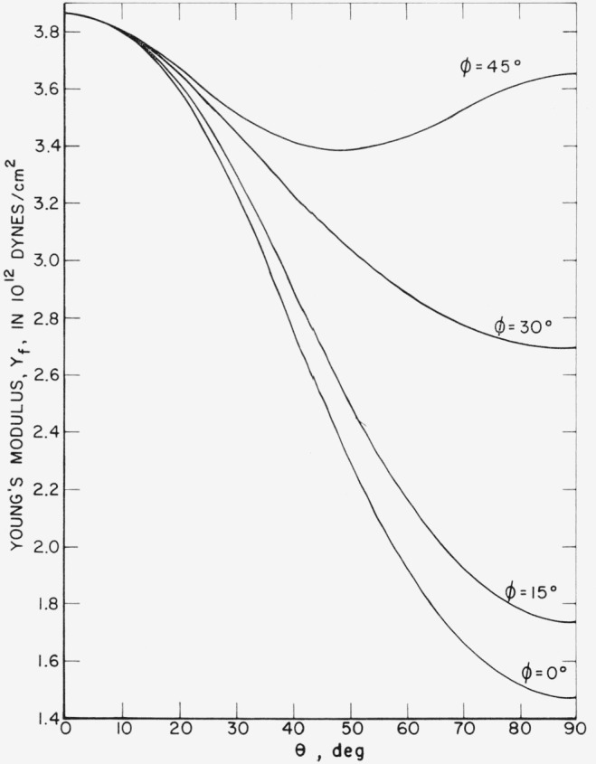
Young’s modulus, Yf, as a function of orientation, calculated from eqs (1) and (6), using the least squares best estimates of the coefficients given in table 4.
Figure 3.

Shear modulus, Gf, as a function of orientation, calculated from eqs (2) and (7), using the least squares best estimates of the coefficients given in table 4.
The writers have previously used the resonance method to determine the six elastic compliances, sij, of corundum [11] with standard deviations of about 0.1 percent for the diagonal compliances and about 1.0 percent for the off-diagonal compliances. The present uncertainties in the diagonal constants range from 0.2 percent for s11 to 2.6 percent in s66. For the off-diagonal constants the values are 1.7 percent for s12 and 4.3 percent for s13. These results are somewhat disappointing when compared with the precision achieved with corundum. Rutile differs from corundum in being more anisotropic but this should not cause such an increase in standard deviation if the orientation were constant throughout the specimen. The principal difficulty probably is associated with the small angle boundaries. If specimens free of these boundaries are ever produced it would be interesting to repeat both the pulse velocity and resonance measurements and attempt to obtain agreement to 0.1 percent in the diagonal constants. It is probably not worthwhile to attempt to improve the agreement using existing specimens. The present results are accurate enough for most purposes and the general agreement of different observers leaves no question of serious error. The value of c33 calculated by Dayal and Appalanara-simham from spectroscopic data is in serious error, as previously noted [9, 10], and an extension of their calculation to correct this value might be worthwhile.
Acknowledgments
The writers gratefully acknowledge the help provided by the suppliers of the rutile powder and single crystals. In particular we thank W. S. Brower and S. F. Holley of the National Bureau of Standards, R. G. Rudness of the Linde Co., and M. D. Beals of the National Lead Co.
Footnotes
Italicized figures in brackets indicate the literature references at the end of this paper.
A division of Union Carbide and Carbon Co.
This equation should not be confused with an approximate differential equation derived by Timoshenko [19] and studied by Goens [20] and by Pickett [21].
Note.—The writers were recently informed by Gilman [27] of unpublished work by himself and B. Chick on the elastic constants of rutile. They obtained c33=4.75×10¹² dynes/cm2 and c44= 1.23×10¹² dynes/cm2. Both values are in good agreement with the results of the present work.
7. References
- 1.Grant FA. Properties of rutile (titanium dioxide) Revs Modern Phys. 1959;31:646–764. [Google Scholar]
- 2.Frederikse HPR. Recent studies on rutile (TiO2) J Appl Phys Suppl. 1961;32:2211–2215. [Google Scholar]
- 3.Hollander LE, Jr, Castro PL. Lockheed Technical Report LMSD–894803. 1961. Bibliography and technical review of rutile. Astia number 257867. [Google Scholar]
- 4.Bridgman PW. The linear compressibility of thirteen natural crystals. Am J Sci. 1928;15:287. [Google Scholar]
- 5.Dayal B, Appalanarasimham N. The evaluation of the elastic constants of rutile from spectroscopic data. J Sci Res of Benares Hindu Univ. 1950;1:26–30. [Google Scholar]
- 6.Vick GL, Hollander LE, Brown AE. Elastic moduli of single-crystal rutile (TiO2) Bull Am Phys Soc Ser II. 1959;4:463. [Google Scholar]
- 7.Verma RK. Elasticity of some high density crystals. J Geophys Res. 1960;65:757–766. [Google Scholar]
- 8.Wachtman JB, Jr, Tefft WE, Lam DG., Jr Elastic constants of rutile (TiO2) Bull Am Phys Soc Ser II. 1960;5:278. [Google Scholar]
- 9.Vick GL, Hollander LE. Ultrasonic measurement of the elastic moduli of rutile. J Acoust Soc Am. 1960;32:947. [Google Scholar]
- 10.Birch Francis. Elastic Constants of Rutile—A correction to a paper by R. K. Verma, “Elasticity of Some High-Density Crystals,”. J Geophys Res. 1960;65:3855–3856. [Google Scholar]
- 11.Wachtman JB, Jr, Tefft WE, Lam DG, Jr, Stinchfield RP. Elastic constants of synthetic single crystals corundum at room temperature. J Research NBS. 1960;64A:213–228. doi: 10.6028/jres.064A.022. [DOI] [PMC free article] [PubMed] [Google Scholar]
- 12.Wachtman JB, Jr, Doyle LR. Related effects of point defects on electrical and mechanical properties of nonmetallic crystalline solids. J Am Ceram Soc submitted to. [Google Scholar]
- 13.Brown WF., Jr Interpretation of torsional frequencies of crystal specimens. Phys Rev. 1940;58:998–1001. [Google Scholar]
- 14.Nye JF. Physical properties of crystals. Oxford Univ. Press; London, England: 1957. [Google Scholar]
- 15.Hearmon RFS. The elastic constants of anisotropic materials. Rev Mod Phys. 1946;18:409–440. [Google Scholar]; The elastic constants of anisotropic materials II. Adv in Phys. 1956;5:323–382. [Google Scholar]
- 16.Rayleigh Lord. The theory of sound. Vol. 1. Dover Publications; New York, N.Y.: 1945. p. 251. [Google Scholar]
- 17.Bancroft Dennison. The velocity of longitudinal waves in cylindrical bars. Phys Rev. 1941;59:588–293. [Google Scholar]
- 18.Pickett Gerald. Flexural vibration of unrestrained cylinders and discs. J App Phys. 1945;16:821. [Google Scholar]
- 19.Timoshenko SP. On the correction for shear of the differential equation for transverse vibrations of prismatic bars. Phil Mag. 1921;41:744–746. [Google Scholar]; On the transverse vibrations of bars of uniform cross-section. Phil Mag. 1922;43:125–131. [Google Scholar]
- 20.Goens E. Uber die Bestimmung des Elastizitats moduls von Staben mit Hilfe von Biegungsschwingungen. Ann Physik. 1931;11:649–768. [Google Scholar]
- 21.Pickett Gerald. Equations for computing elastic constants from flexural and torsional resonant frequencies of vibration of prisms and cylinders. Proc ASTM. 1945;45:846–865. Also available as Bull. 7 of the Research Lab. of Portland Cement Assoc. [Google Scholar]
- 22.Tefft WE. Numerical solution of the frequency equations for the flexural vibration of cylindrical rods. J Research NBS. 1960;64B:237–242. [Google Scholar]
- 23.Spinner S, Tefft WE. A Method for determining mechanical resonance frequencies and for calculating elastic moduli from these frequencies. Proc ASTM. 1961;61:1221–1237. [Google Scholar]
- 24.Swanson HE. Eleanor Tatge, Standard X-ray diffraction powder patterns. NBS Circ. 1953;I:539. [Google Scholar]
- 25.Scheffe H. The analysis of variance. John Wiley & Sons; New York, N.Y.: 1959. [Google Scholar]
- 26.Huntington HB. Solid State Phys. Vol. 7. Academic Press; New York, N.Y.: 1958. The elastic constants of crystals; pp. 213–351. [Google Scholar]
- 27.J. J. Gilman, Brown University Private communication.