

Abstract
The frequencies of the vibration-rotation spectrum of N2O have been measured from 1830 cm−1 to 2270 cm−1. A number of weak bands have been measured and assigned to “hot bands’’ and isotopic species in normal abundance. By using the Ritz principle and previously measured bands the bending frequency (v2) is calculated as 588.780 cm−1. Frequencies are given for lines arising from the three principal transitions found in this region.
1. Introduction
Recently there has been considerable interest in obtaining accurate values for the vibration-rotation potential constants for small molecules. Pliva [1]1 has measured the spectra of various isotopic species of nitrous oxide (N2O) in the hope of obtaining more data with which to check the anharmonic terms of a potential function which he has devised [2]. Tidwell, Plyler, and Benedict [3] have reported measurements on a large number of vibrational-energy levels for N2O and have derived a set of vibration-rotation constants.
Rank et al. [4] have reported the results of some very precise measurements on five absorption bands of N2O. McCubbin, Grosso, and Mangus [5] have made some further precise measurements on N2O which will be reported soon. While this work was in progress Fraley, Brim, and Rao [6] published results of measurements on the strongest absorption lines due to N2O in the 5-μ region. The latter measurements are in essential agreement with those reported here.
2. Experimental Procedure
The spectra were measured on the NBS high-resolution infrared spectrometer described elsewhere [7]. Most of the measurements were made using a 7,500 lines/in. grating although some measurements were obtained with a 1,860 lines/in. grating. A liquid-nitrogen cooled PbSe detector was used. Calibration was achieved by the combination of accurately measured rare-gas spectra and a Fabry-Perot interferometer fringe system in the manner described in reference 8.
Spectra were obtained with pathlengths of 1.2, 4, and 24 m and pressures ranging from 1 to 200 mm Hg. Representative spectra are shown in figures 1 and 2. The 1.2 m cell could be either cooled to 220 °K or warmed to 400 °K; representative spectra obtained at these temperature extremes are shown in figures 3 and 4. In these figures it is evident that many lines which are weak at low temperatures have intensified with increase in temperature. These lines must be attributed to transitions originating from excited vibrational states and accordingly have been assigned as “hot band” lines.
Figure 1. N2O absorption from 1840 to 1910 cm−1.

Pathlength 1.2 m; pressure 28 cm Hg.
Figure 2. N2O absorption from 2270 to 2160 cm−1.

Pathlength 4 m; pressure 1 mm Hg. Circle: indicates absorption lines due to atmospheric C13O216 in the optical path.
Figure 3. N2O absorption from 2184 to 2200 cm−1.
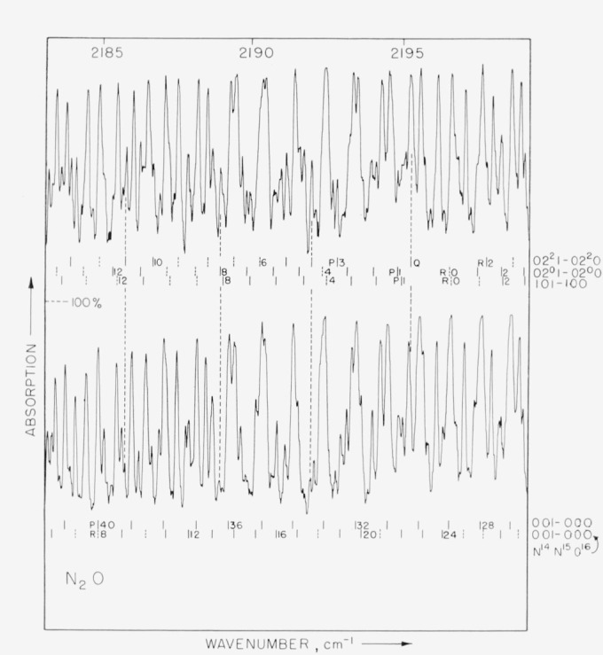
Upper curve is for a temperature of 400 °K and lower curve is with cell cooled to about 220 °K. Pathlength is 1.2 m; pressure 1 mm Hg.
Figure 4. N2O absorption from 2204 to 2220 cm−1.
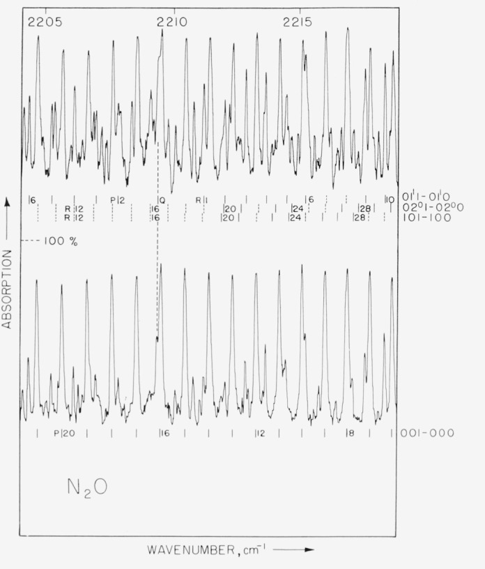
Temperature of gas in upper eurve is 400 °K, temperature of gas in lower curve is 220 °K. Pathlength is 1.2 m; pressure is 2 mm Hg.
3. Analysis of Data
The microwave measurements of Burrus and Gordy [9] have given very precise values for the ground-state rotational constant, B0, and the l-doubling constant, q, of the molecule N14N14O16. Coles and Hughes [10] and Coles, Good, and Lide [11] have made further measurements from which one can obtain B0 for the isotopes N14N15O16, N15N14O16, and N14N14O18. Combining the results of these workers with the velocity of light (taken as 299,793 km/s) we have calculated these constants in wavenumbers as given in table 1. Since these molecular constants are more accurate than could be obtained from the measurements reported here, the values given in table 1 were used wherever applicable for the calculation of the other molecular constants. For this same purpose the value of D0 = 17.6×10⁻⁸ cm−1 given by Rank et al. [4] was used.
Table 1.
Accurately known molecular constants used in the analysis of the N2O hands between 4.4 and 5.5 μ
| B000 = 0.4190104 cm−1 |
| D000 = 17.6×10⁻⁸ cm−1 |
| q = 79.17×10⁻⁵ cm−1 |
| B010 = 0.4195727 cm−1 (average of c and d levels) |
| B000(N14N15O16) =0.4189821 cm−1 |
| B000(N15N14O16) = 0.4048564 cm−1 |
| B000(N14N14O18) =0.395577 cm−1 |
Since the data for many of the bands reported here was rather fragmentary due to the high degree of overlapping, all of the absorption bands were analyzed by obtaining a least-squares fit to the polynomial
where the terms have their usual significance.
The data were also analyzed using the method of combinations and differences. The results of both methods were comparable, but in many cases the fact that more lines could be used in fitting to the polynomial given above resulted in a reduction in the uncertainty of the various unknown constants when this method was used, especially since the lower state constants were in most cases very accurately known.
For those bands which are split into resolved c and d components the two bands were analyzed simultaneously to obtain a least-squares fit to the same band center and other constants were made compatible. A more detailed description is given for the individual bands in the next section.
4. Results
4.1. The Region From 1830 to 1925 cm−1
In this region lines have been identified due to the three transitions 12°0–01lc0, 1220–0110, and 111c0– 000. For all these perpendicular bands the Q branches were observed, but the resolution was not good enough to measure any individual Q branch lines. The splitting of the Δ—II band was observed for all but a few low J lines. The analysis of this Δ—II band was carried out by analyzing the c and d components simultaneously. Since the data were quite fragmentary for these weak “hot bands,” the best available estimates of the values of , , D″, , and were used in order to obtain more accurate values of v0 and B′. For this purpose it was assumed that . Since the c and d levels of the 1220 state undergo l-type resonance with different levels, it was necessary to use different values of D for the c and d levels. The values of the constants used are given in table 2. Only the c component of the v1 + v2 band was measured, therefore the value obtained for ΔB as given in table 2 is for the transition to the c level only.
Table 2. Vibration-rotation constants describing the absorption bands of N2O in the 2000 cm−1 Region.
The limits of error given are standard deviations
| Isotopic species | Assignment | v0 | ΔB×10+5cm−1 | *D′ × 108 | *D″ × 108 | ΔD × 10+8 |
|---|---|---|---|---|---|---|
|
|
|
|
|
|
|
|
| N14N14O16 | 1200–011c0 | 1873.206 ±0.009 | −93**±3 | 23.8 | 17.6 | ….. |
| 111c0–000 | 1880.271 ±.003 | −154. 6±0.7 | 17.6 | 17.6 | −0.2±0.3 | |
| 122c0–011c0 | }1886.033 ± 00.9 | − 96 ± 3 | }17.6 | ….. | ||
| 122d0–011d0 | ||||||
| 200–011c0 | }1974.571 ± .003 | − 397. 5 ± 1.0 | 16.1 | 17.6 | − 2.3±0.6 | |
| 200–011d0 | ||||||
| 2110–0220 | 1988.2±.3 — Q branch position | |||||
| 211d0–0200 | 1997.65 ± .15 —Q branrh position | |||||
| 022cl–022c0 | }2195.406 ± .006 | − 340. 3± 1.2 | 11.6 | ….. | ||
| 022d1–022d0 | 17.6 | ….. | ||||
| 020l–0200 | 2195.849±.025 | −336±2 | 23.6 | 23.6 | 0±1.4 | |
| 101–100 | 2195.93±.04 | −352 ± 5 | 17.0 | 17.4 | ….. | |
| O111–0110 | 2209.527±.004 | −340. 3 ± 0.9 | 17.6 | 17.6 | 0.4±0.3 | |
| 001–000 | 2223.764 ± .003 | −345.6±0.3 | 17.4 | 17.6 | −.26±0.05 | |
| N14N15O16 | 0111–0110 | 2164.13 ± .03 | −315 ± 15 | 17.5 | 17.5 | ….. |
| N14N15O16 | 001–000 | 2177.659 | −330 ± 3 | 17.5 | 17.5 | ….. |
| N15N14O16 | 001–000 | 2201.604±.015 | −337 ±3 | 16.5 | 16.5 | ….. |
| N14N14O18 | 001–000 | 2219.678 ±.02 | −411±10 | 16.5 | 16.5 | ….. |
In all cases the values of D given were assumed in order to obtain the best possible values of v0, ΔB, and ΔD.
This ΔB value is from the average of the c and d levels of the lower state.
The calculated and observed frequencies of absorption lines due to the transition 111c0–000 are given in table 3. Figure 1 shows the appearance of the absorption in this region.
Table 3.
Observed and calculated wavenumbers for the two strongest N2O absorption bands between 1830 and 2000 cm−1
| J″ | 111c 0–000
|
200–011c 0
|
200–011d 0
|
|||||||
|---|---|---|---|---|---|---|---|---|---|---|
|
P
|
R
|
P
|
R
|
Q
|
||||||
| Obs. | Calc. | Obs. | Calc. | Obs. | Calc. | Obs. | Calc. | Obs. | Calc. | |
|
|
|
|
|
|
|
|
|
|
|
|
| 0 | ….. | ….. | 1881.095 | .106 | ….. | ….. | ….. | ….. | ….. | ….. |
| 1 | ….. | ….. | 81.929 | .937 | ….. | ….. | b1976.222 | .227 | ….. | ….. |
| 2 | b1878.595 | .591 | 82.751 | .766 | ….. | ….. | ….. | ….. | ….. | ….. |
| 3 | b77.766 | .747 | 83.600 | .592 | ….. | ….. | b77.832 | .853 | ….. | ….. |
| 4 | 76.894 | .900 | ….. | ….. | ….. | ….. | b78.643 | .656 | ….. | ….. |
| 5 | 76.041 | .050 | ….. | ….. | ….. | ….. | ….. | ….. | ….. | ….. |
| 6 | 75.185 | .196 | ….. | ….. | ….. | ….. | b80.253 | .239 | ….. | ….. |
| 7 | ….. | ….. | 86.865 | .863 | ….. | ….. | 81.016 | .020 | ….. | ….. |
| 8 | b73.472 | .480 | ….. | ….. | ….. | ….. | 81.790 | .794 | ….. | ….. |
| 9 | ….. | ….. | ….. | ….. | b1960.764 | .769 | 82.559 | .561 | ….. | ….. |
| 10 | ….. | ….. | ….. | ….. | b65.880 | .867 | 83.317 | .320 | ….. | ….. |
| 11 | ….. | ….. | ….. | ….. | 64.952 | .957 | 84.081 | .073 | 1973.995 | .995 |
| 12 | ….. | ….. | b90.861 | .882 | 64.034 | .040 | 84.821 | .818 | ….. | ….. |
| 13 | ….. | ….. | b91.684 | .677 | 63.127 | .117 | 85.553 | .556 | 73.784 | .777 |
| 14 | ….. | ….. | b92.488 | .468 | 62.181 | .186 | 86.287 | .287 | 73.636 | .655 |
| 15 | ….. | ….. | 93.253 | .256 | ….. | ….. | 87.030 | .010 | 73.543 | .524 |
| 16 | ….. | ….. | 94.054 | .041 | 60.302 | .303 | 87.723 | .727 | 73.400 | .384 |
| 17 | b65.590 | .607 | b94.850 | .823 | 59.351 | .351 | ….. | ….. | 73.218 | .236 |
| 18 | b64.720 | .717 | b95.585 | .601 | 58.399 | .392 | 89.127 | .139 | 73.088 | .079 |
| 19 | b63.844 | .824 | ….. | ….. | 57.422 | .426 | 89.833 | .834 | 72.920 | .914 |
| 20 | b62.958 | .928 | 97.150 | .149 | 56.448 | .453 | 90.521 | .522 | 72.754 | .740 |
| 21 | ….. | ….. | 97.910 | .918 | 55.465 | .473 | ….. | ….. | 72.560 | .557 |
| 22 | 61.130 | .128 | 98.674 | .684 | 54.494 | .489 | ….. | ….. | 72.381 | .366 |
| 23 | 60.210 | .223 | 1899.436 | .447 | 53.490 | .493 | ….. | ….. | 72.160 | .166 |
| 24 | 59.315 | .315 | b1900.190 | .207 | 52.487 | .4.92 | 93.222 | .202 | b71.986 | .957 |
| 25 | ….. | ….. | 00.964 | .963 | 51.481 | .484 | 93.859 | .855 | 71.746 | .740 |
| 26 | 57.496 | .491 | 01.715 | .716 | 50.469 | .470 | 94.496 | .500 | 71.518 | .514 |
| 27 | 56.576 | .574 | b02.493 | .466 | b49.440 | .449 | 95.138 | .138 | b71.258 | .280 |
| 28 | 55.662 | .654 | 03.221 | .213 | 48.423 | .420 | 95.777 | .770 | b71.032 | .037 |
| 29 | 54.739 | .732 | 03.960 | .957 | 47.383 | .386 | 96.389 | .394 | 70.787 | .786 |
| 30 | 53.808 | .806 | 04.689 | .697 | ….. | ….. | ….. | ….. | 70.518 | .526 |
| 31 | 52.884 | .877 | 05.425 | .435 | ….. | ….. | b97.600 | .621 | b70.270 | .258 |
| 32 | 51.950 | .946 | 06.154 | .169 | 44.234 | .240 | b1998.197 | .224 | 69.987 | .981 |
| 33 | 51.012 | .012 | 06.883 | .900 | b43.171 | .178 | 1969.700 | .696 | ||
| 34 | 50.062 | .074 | b07.617 | .627 | ….. | ….. | ||||
| 35 | 49.125 | .134 | 08.348 | .352 | 41.034 | .033 | ||||
| 36 | ….. | ….. | 09.070 | .073 | 39.938 | .951 | ||||
| 37 | b47.256 | .245 | ….. | ….. | 38.880 | .862 | ||||
| 38 | b46.266 | .296 | 10.517 | .506 | b37.783 | .767 | ||||
| 39 | ….. | ….. | 11.220 | .217 | 36.680 | .665 | ||||
| 40 | ….. | ….. | 11.931 | .926 | 35.542 | .556 | ||||
| 41 | ….. | ….. | 12.626 | .631 | 1934.443 | .441 | ||||
| 42 | b42.475 | .472 | 13.345 | .333 | ||||||
| 43 | 41.518 | .509 | 14.024 | .032 | ||||||
| 44 | 40.544 | .543 | b14.720 | .727 | ||||||
| 45 | b39.591 | .574 | 1915.421 | .420 | ||||||
| 46 | 38.604 | .602 | ||||||||
| 47 | ….. | ….. | ||||||||
| 48 | 36.662 | .650 | ||||||||
| 49 | 35.672 | .670 | ||||||||
| 50 | 34.696 | .687 | ||||||||
| 51 | 33.700 | .701 | ||||||||
| 52 | 32.712 | .712 | ||||||||
| 53 | b1831.720 | .721 | ||||||||
Blended or weak lines.
4.2. Absorption Lines in the Region 1925 to 2000 cm−1
The main band found in this region is a Σ–II band due to the transition 200–0110. In this case the Q branch was sufficiently well resolved so that measurements were obtained for both the c and d levels. Since microwave values for the lower state are quite good, these values were used in the analysis and transitions from both the c and d levels were analyzed simultaneously by a least-squares program in order to obtain the best values for v0 and B′.
Absorption in this region was very weak as might be expected from the transitions involved. The Q branches for the two “hot bands” 2110–0220 and 2110–0200 were also observed in this wavelength region, but they were not resolved. Nor were any lines of the P and R branches observed.
The calculated and observed frequencies of the lines for the 200–0110 transition are given in table 3.
4.3. N14N14O16 Absorption Between 2130 and 2270 cm−1
The fundamental v3 and associated “hot bands” are located in this region. v3 is a rather strong absorption band, consequently with the pathlength and resolution available it was possible to obtain measurements on four “hot bands” and four isotopic bands.
The splitting of the first “hot band” was observed for high-J levels but overlapping with various other bands was rather severe. For this reason it was felt that more accurate band constants could be obtained by averaging the frequencies of the c and d components. Even though this procedure did not permit the use of measurements where only one component was observed, the resultant constants are believed to be more reliable than those found by analyzing each band individually.
Lines due to the Δ—Δ transition 0221–0220 have been observed and the position of the Q, while overlapped, has been verified by observations at 220 °K and 400 °K. Figure 3 shows a few lines due to this transition and the manner in which the line intensities change with temperature. The Boltzman distribution predicts this transition will show an approximate six-fold increase in intensity in going from 220 °K to 400 °K.
Since the two Σ—Σ transitions 101–100 and 0201–0200 are predicted to lie quite close to each other, some difficulty was anticipated in assigning the two series of lines which must be due to these transitions. The assignments of these lines are, however, considered to be reliable due to the rather large differences in the lower-state B values. Δ2F″ plots for these two bands yield respective B″ values of 0.4175 and 0.4200 cm−1. The B″ values expected from the data of reference 3 are 0.41725 and 0.41991, respectively. Many of the low-J lines are badly overlapped because the two band centers lie so close together. As a consequence the band centers calculated from the data may be in error by several hundredths of a wavenumber. The statistical treatment of the data resulted in a standard deviation for the v0 values of 0.01 cm−1, but inspection of the data leads us to believe that this is not a realistic number. Therefore table 2 contains a more subjective evaluation of the accuracy of the band centers for these two bands.
Table 4 lists the frequencies of the v3 band as observed in this laboratory and as reported by Fraley, Brim, and Rao. Columns 3 and 6 compare the calculated frequencies with those observed.
Table 4.
Wavenumbers of absorption lines for the v1 band of N2O
| J |
P Branch
|
R Branch
|
||||
|---|---|---|---|---|---|---|
| Observed wavenumber NBS | Calc.NBS | Observed wavenumber ref. 6 | Observed wavenumber NBS | Calc.NBS | Observed wavenumber ref. 6 | |
|
|
|
|
|
|
|
|
| 0 | ….. | ….. | ….. | 2224.593 | 2224.595 | 2224.594 |
| 1 | b2222.900 | 2222.926 | 2222.940 | b25.41 | 25.419 | 25.430 |
| 2 | b22.065 | 22.081 | 22.085 | b26.237 | 26.236 | 26.243 |
| 3 | b21.253 | 21.229 | 21.273 | (b) | 27.050 | |
| 4 | 20.360 | 20.370 | 20.382 | 27.845 | 27.850 | 27.848 |
| 5 | 19.514 | 19.505 | 19.516 | 28.650 | 28.647 | 28.639 |
| 6 | 18.638 | 18.632 | 18.641 | b29.459 | 29.436 | 29.450 |
| 7 | 17.745 | 17.753 | 17.756 | b30.224 | 30.219 | 30.218 |
| 8 | b16.833 | 16.867 | 16.840 | b30.975 | 30.995 | 30.975 |
| 9 | b15.975 | 15.973 | 15.983 | 31.784 | 31.763 | 31.741 |
| 10 | b15.109 | 15.073 | 15.088 | 32.543 | 32.525 | 32.548 |
| 11 | 14.175 | 14.166 | 14.173 | (b) | 33.301 | |
| 12 | 13.244 | 13.253 | 13.269 | b34.024 | 34.028 | 34.023 |
| 13 | 12.304 | 12.332 | 12.330 | 34.784 | 34.769 | 34.806 |
| 14 | 11.404 | 11.405 | 11.420 | 35.526 | 35.503 | 35.509 |
| 15 | b10.469 | 10.470 | 10.478 | b36.253 | 36.229 | 36.246 |
| 16 | (b) | ….. | 09.523 | b36.942 | 36.950 | 36.945 |
| 17 | b08.582 | 08.581 | 08.590 | b37.670 | 37.663 | 37.663 |
| 18 | 09.625 | 07.626 | 07.622 | 38.364 | 38.369 | 38.368 |
| 19 | 06.669 | 06.665 | 06.668 | b39.076 | 39.068 | 39.076 |
| 20 | 05.681 | 05.696 | 05.687 | b39.728 | 39.760 | 39.761 |
| 21 | 04.719 | 04.721 | 04.717 | 40.454 | 40.445 | 40.444 |
| 22 | b03.737 | 03.739 | 03.735 | 41.134 | 41.123 | 41.130 |
| 23 | b02.736 | 02.750 | 02.741 | 41.780 | 41.794 | 41.805 |
| 24 | b2201.747 | 2201.754 | 01.752 | 42.466 | 42.458 | 42.443 |
| 25 | ….. | ….. | 2200.772 | 43.122 | 43.115 | 43.120 |
| 26 | 2199.720 | 2199.742 | 2199.735 | 43.759 | 43.765 | 43.773 |
| 27 | 98.726 | 98.726 | 98.735 | 44.424 | 44.409 | 44.416 |
| 28 | 97.707 | 97.704 | 97.696 | 45.043 | 45.045 | 45.049 |
| 29 | 96.677 | 96.674 | 96.667 | b45.668 | 45.674 | 45.688 |
| 30 | 95.645 | 95.638 | 95.631 | ….. | ….. | 46.289 |
| 31 | 94.600 | 94.594 | 94.602 | 46.895 | 46.911 | 46.918 |
| 32 | b93.526 | 93.545 | 93.528 | 47.531 | 47.519 | 47.509 |
| 33 | (b) | ….. | 92.428 | 48.114 | 48.120 | 48.119 |
| 34 | b91.432 | 91.425 | 91.433 | 48.712 | 48.714 | 48.714 |
| 35 | b90.345 | 90.355 | 90.349 | 49.304 | 49.301 | 49.328 |
| 36 | 89.264 | 89.278 | 89.280 | 49.887 | 49.881 | 49.889 |
| 37 | 88.184 | 88.194 | 88.189 | 50.460 | 50.454 | 50.449 |
| 38 | 87.134 | 87.104 | 87.106 | 51.033 | 51.020 | 51.047 |
| 39 | 86.002 | 86.007 | 86.004 | (b) | ….. | ….. |
| 40 | 84.911 | 84.903 | 84.890 | 52.145 | 52.131 | 52.148 |
| 41 | 83.794 | 83.793 | 83.790 | 52.682 | 52.676 | 52.685 |
| 42 | 82.666 | 82.676 | 82.667 | 53.209 | 53.214 | 53.216 |
| 43 | b81.560 | 81.552 | 81.545 | (b) | ….. | ….. |
| 44 | (b) | ….. | 80.380 | 54.236 | 54.268 | 54.253 |
| 45 | b79.303 | 79.285 | 79.293 | 54.796 | 54.785 | 2254.799 |
| 46 | (b) | ….. | 78.142 | 55.318 | 55.295 | ….. |
| 47 | 76.982 | 76.991 | 76.983 | 55.796 | 55.797 | ….. |
| 48 | 75.840 | 75.834 | 75.838 | 56.287 | 56.293 | |
| 49 | 74.674 | 74.670 | 74.672 | 56.762 | 56.781 | ….. |
| 50 | 73.497 | 73.500 | 73.488 | b57.300 | 57.263 | ….. |
| 51 | ….. | ….. | 72.324 | b57.707 | 57.737 | ….. |
| 52 | 71.144 | 71.139 | 71.134 | 58.212 | 58.205 | ….. |
| 53 | b69.898 | ….. | 69.891 | 58.664 | 58.665 | ….. |
| 54 | 68.751 | 68.752 | 68.759 | 59.131 | 59.119 | ….. |
| 55 | 67.536 | 67.549 | 2167.579 | (b) | ….. | ….. |
| 56 | b66.318 | 66.339 | ….. | 60.001 | 60.004 | ….. |
| 57 | (b) | ….. | ….. | 60.419 | 60.436 | ….. |
| 58 | 63.926 | 63.900 | ….. | 60.882 | 60.862 | ….. |
| 59 | 62.690 | 62.670 | ….. | b61.28 | 61.280 | ….. |
| 60 | 61.418 | 61.434 | ….. | 61.675 | 61.691 | ….. |
| 61 | 60.210 | 60.191 | ….. | 62.082 | 62.095 | ….. |
| 62 | 58.979 | ….. | ….. | 62.489 | 62.492 | ….. |
| 63 | 57.693 | 57.686 | ….. | (b) | ….. | ….. |
| 64 | 56.422 | 56.424 | ….. | ….. | ….. | ….. |
| 65 | 55.168 | 55.155 | ….. | 63.636 | 63.640 | ….. |
| 66 | 53.883 | 53.880 | ….. | 64.020 | 64.009 | ….. |
| 67 | ….. | ….. | ….. | 64.362 | 64.371 | ….. |
| 68 | 51.295 | 51.310 | ….. | 64.741 | 64.725 | ….. |
| 69 | b49.976 | 50.015 | ….. | (b) | ….. | ….. |
| 70 | 48.740 | 48.714 | ….. | 65.429 | 65.414 | ….. |
| 71 | 47.369 | 47.406 | ….. | (b) | ….. | |
| 72 | 46.097 | 46.092 | ….. | b66.08 | 66.074 | ….. |
| 73 | 44.736 | 44.771 | ….. | b66.40 | 66.393 | ….. |
| 74 | b43.46 | 43.444 | ….. | b66.713 | 66.705 | ….. |
| 75 | (b) | ….. | ….. | (b) | ….. | ….. |
| 76 | (b) | ….. | ….. | (b) | ….. | ….. |
| 77 | b39.438 | 39.424 | ….. | b2267.612 | 2267.600 | ….. |
| 78 | b2138.086 | 2138.072 | ….. | ….. | ….. | ….. |
Blended or weak lines.
4.4. Isotopic Absorption Bands From 2100 to 2240 cm−1
Within this region absorption bands due to N2O molecules containing N15 or O18 are expected. Lines due to four transitions in such isotopically substituted molecules have been identified in this study.
The band at 2201.60 cm−1 due to N15N14O16 has been previously measured by Pliva [1] but bands due to the molecules N14N15O16 and N14N14O18 found at 2164.13, 2177.66, and 2219.67 cm−1 have not been previously reported. The assignments for these latter three bands have been confirmed by determination of the values of B″ from the Δ2F″ plots. In the case of the II—II transition at 2164.13 cm−1 the sharp Q branch seems to be observable at 2164.128 cm−1, thus providing greater confidence in the position of the band center. Since many of the lines for these isotopic molecules were weaker than or of comparable intensity with the “hot bands” of the most abundant molecule, the identification of the lines was greatly aided by spectra obtained at 220 °K. At this temperature the intensity of the “hot band” lines is very greatly diminished. This leaves the isotopic lines as the most outstanding of the weak lines at low temperatures.
4.5. Discussion of Results
By means of the Ritz principle the position of some of the low-lying vibrational levels may be obtained. The bending vibration, v2, may be obtained in four different ways. Using the precise measurements of reference 4 and the recent measurements of reference 5, we find
Taking the average of the values given for the 0111–000 transition in references 1 and 3, one obtains
The average of these four indirect determinations, 588.780 cm−1, compares very favorably with the indirect measurement of Pliva [1] (588.767 cm−1), the four indirect measurements of Tidwell et al. [3] (588.773 cm−1), and the direct measurement of Lakshmi, Rao, and Nielsen [12] (588.78 cm−1).
The Ritz principle may also be applied to determine the values of , and v1 as follows:
where the values for the vibration levels given by Pliva [1] and Tidwell et al. [3] are used. By using similar combinations Tidwell et al., have previously determined . McCubbin et al. [5] have recently measured and v1 at 1168.134 and 1284.907 cm−1, respectively. These were direct measurements and should be more accurate than the indirectly obtained values given above.
The band centers for the transitions 001–000 and 0111–0110 have now been measured quite carefully in three different laboratories. Some idea of the absolute accuracy of these measurements may be obtained by comparing the constants derived from the measurements. We may also compare the measurements of v3 for the N15N14O16 molecule with those reported by Pliva [1]. Table 5 shows how closely these independent measurements agree. Although it is seen that Pliva and Fraley et al., agree on a slightly larger value for B001 than has been reported in this work, nevertheless it is felt that the values given here are probably more accurate. The present measurements extend to considerably higher values of J than previous measurements and as a consequence a more accurate determination of ΔB and ΔD is expected. On the other hand Fraley, Brim, and Rao probably have a more accurate value for v0 since their resolution was slightly better so that blending of low-J lines would have less tendency to cause errors in the derived v0. Since Pliva worked with an isotopically enriched sample, it is to be expected that his constants for N15N14O16 are better than those reported here.
Table 5.
Comparison of the results of measurements on N2O in different laboratories
An attempt was made to compare the results of this work with the constants given by Tidwell et al., but, as noted by Pliva [1], the agreement is not entirely satisfactory. Perhaps the measurements given here will be of value in determining the accuracy of the revised constants which Pliva is calculating.
Footnotes
This work was supported in part by the Geophysic Research Directorate, Air Force Cambridge Research Laboratories.
Figures in brackets indicate the literature references at the end of this paper.
5. References
- 1.Pliva Josef. International Symposium on Molecular Structure and Spectroscopy. Tokyo, Japan: Sept. 1962. [Google Scholar]
- 2.Pliva Josef. Collection Czech Chem Communs. 1958;23:777. [Google Scholar]
- 3.Tidwell ED, Plyler EK, Benedict WS. J Opt Soc Am. 1960;50:1243. [Google Scholar]
- 4.Rank DH, Eastman DP, Rao BS, Wiggins TA. J Opt Soc Am. 1961;51:929. [Google Scholar]
- 5.McCubbin TK, Grosso R, Mangus J. to be published [Google Scholar]
- 6.Fraley PE, Brim WW, Rao KN. J Mol Spect. 1962;9:487. [Google Scholar]
- 7.Plyler EK, Blaine LR. J Res NBS. 1959;62(1):7. Phys and Chem. [Google Scholar]
- 8.Plvler EK, Blaine LR, Tidwell ED. J Res NBS. 1955;55:279. RP2630. [Google Scholar]
- 9.Burrus CA, Gordy W. Phys Rev. 1956;101:599. [Google Scholar]
- 10.Coles DK, Hughes RH. Phys Rev. 1949;76:178A. [Google Scholar]
- 11.Kislink P, Townes CH. NBS Circ. 1952;518 [Google Scholar]
- 12.Lakshmi K, Rao KN, Nielsen HH. J Chem Phys. 1956;24:811. [Google Scholar]