Survival analysis in the presence of competing risks

Abstract

Survival analysis in the presence of competing risks imposes additional challenges for clinical investigators in that hazard function (the rate) has no one-to-one link to the cumulative incidence function (CIF, the risk). CIF is of particular interest and can be estimated non-parametrically with the use cuminc() function. This function also allows for group comparison and visualization of estimated CIF. The effect of covariates on cause-specific hazard can be explored using conventional Cox proportional hazard model by treating competing events as censoring. However, the effect on hazard cannot be directly linked to the effect on CIF because there is no one-to-one correspondence between hazard and cumulative incidence. Fine-Gray model directly models the covariate effect on CIF and it reports subdistribution hazard ratio (SHR). However, SHR only provide information on the ordering of CIF curves at different levels of covariates, it has no practical interpretation as HR in the absence of competing risks. Fine-Gray model can be fit with crr() function shipped with the cmprsk package. Time-varying covariates are allowed in the crr() function, which is specified by cov2 and tf arguments. Predictions and visualization of CIF for subjects with given covariate values are allowed for crr object. Alternatively, competing risk models can be fit with riskRegression package by employing different link functions between covariates and outcomes. The assumption of proportionality can be checked by testing statistical significance of interaction terms involving failure time. Schoenfeld residuals provide another way to check model assumption.

Zhongheng Zhang, MMed.

Introduction

Competing risks arise in clinical research when there are more than one possible outcome during follow up for survival data, and the occurrence of an outcome of interest can be precluded by another. The latter is called the competing risk (1-4). In clinical oncology for example, cancer-related mortality may be of primary interest, but other causes of death can prevent its occurrence and deaths caused by reasons other than cancer are typical examples of competing risks. In critical care researches, investigators may examine different strategies to maintain central venous patency in intensive care unit (ICU) (5,6). Patients in different groups were followed up for the occurrence of lumen non-patency. However, patients may die before the occurrence of lumen non-patency. Death can be considered as censoring and Cox proportional hazard model may be applied to estimate the effect of covariate on hazard. However, the effect on hazard cannot be directly liked to cumulative incidence function (CIF), thus other modeling methods are required. This article will describe different approaches for survival analysis in the presence of competing risks. The basic ideas of each method will be introduced and detailed R code be provided in the main text. I also highlight the interpretation of statistical output produced by R code.

Key concepts in survival analysis with and without competing risks

Survival data can be characterized by hazard function [$h(t)$] which provides a dynamic description of the instantaneous risk of failing given survival until time t. Cumulative hazard function [$H(t)$] is the $h(t)$ added over time from 0 to t. In contrast to $h(t)$, $H(t)$ has no simple probabilistic interpretation. However, a plot of $\widehat{H}(t)$ against t can provide useful information in that its local slope approximates the $h(t)$ (7). Survival function [$\widehat{S}(t)$] can be estimated non-parametrically using Kaplan-Meier estimator, and the $\widehat{H}(t)$ can be estimated using Nelson-Aalen estimator. In the absence of competing risks, there is a one-to-one correspondence between $S(t)$ and $H(t)$:

$$S(t)=e^{-H(t)}$$ [1]

and the CIF is one minus the survival function:

$$F(t)=1-e^{-H(t)}$$ [2]

However, in the presence of competing risks, the CIF cannot be directly linked to the hazard function. Let 1 denote the event of interest and 2 denote the competing risk event. Then cumulative incidence for event of interest can be written as (8):

$$F_1(t)={\displaystyle {\int }_0^{t}S(s)\cdot h_1(s)}\cdot ds$$ [3]

where $S(s)=e^{-H_1(s)-H_2(s)}$ is the survival function at time s and is determined by the both event of interest and competing event. Therefore, there is no one-to-one correspondence between cumulative incidence [$F_1(t)$] and cause-specific hazard [$h_1(s)$]. Cumulative incidence derived from Kaplan-Meier estimator is always larger than that obtained by counting for competing risks. In Kaplan-Meier estimation, an individual is removed from the risk set when the individual experiences competing event. Within competing risk framework, the individual is an event in the calculation of overall survival probability. Therefore, the overall survival [$S(s)$] of any event is lower when competing risks are considered. When event 2 is considered as non-informative censoring in Kaplan-Meier estimator the overall survival will be larger ($e^{-H_1(S)}\ge e^{-H_1(S)}{}^{-H_2(S)}$). If hazard is considered as the rate, cumulative incidence is the risk in epidemiology terms. In competing risk analysis, individuals experiencing the competing risk event have zero probability of experiencing the event of interest. In contrast, the naïve Kaplan-Meier approach assumes that these individuals would experience the same probability of event of interest in pure theory (non-informative censoring). Thus, the latter overestimates the cumulative incidence of the event of interest.

The effect of covariates on hazard rate can be estimated using COX proportional hazard regression model. The exponentiation of the coefficient gives the hazard ratio (HR) which is the ratio of rate in epidemiology. Because hazard function has a one-to-one correspondence to the cumulative incidence, the HR also reflects the risk (cumulative incidence) of the study population. However, this relationship does not exist in the presence of competing risks. Although the cause-specific hazard regression model represents the impact of covariates on the cause-specific hazard, it does not necessarily reflect the impact on the cumulative incidence. Because clinicians or investigators may be interested in both rate and risk, the impact of covariates on both quantities can be reported side-by-side in an article (2). The Fine-Gray model was developed to link covariates to cumulative incidence. The statistics derived from Fine-Gray model are subdistribution hazard ratio (SHR) which is actually not equivalent to the HR in conventional framework (9). I will illustrate it in the following examples.

Worked example

The worked example is contained in the riskRegression package. A total of 205 patients with melanoma had undergone surgical operation and were followed up until the end of 1977. The dataset can be loaded and viewed in the following way.

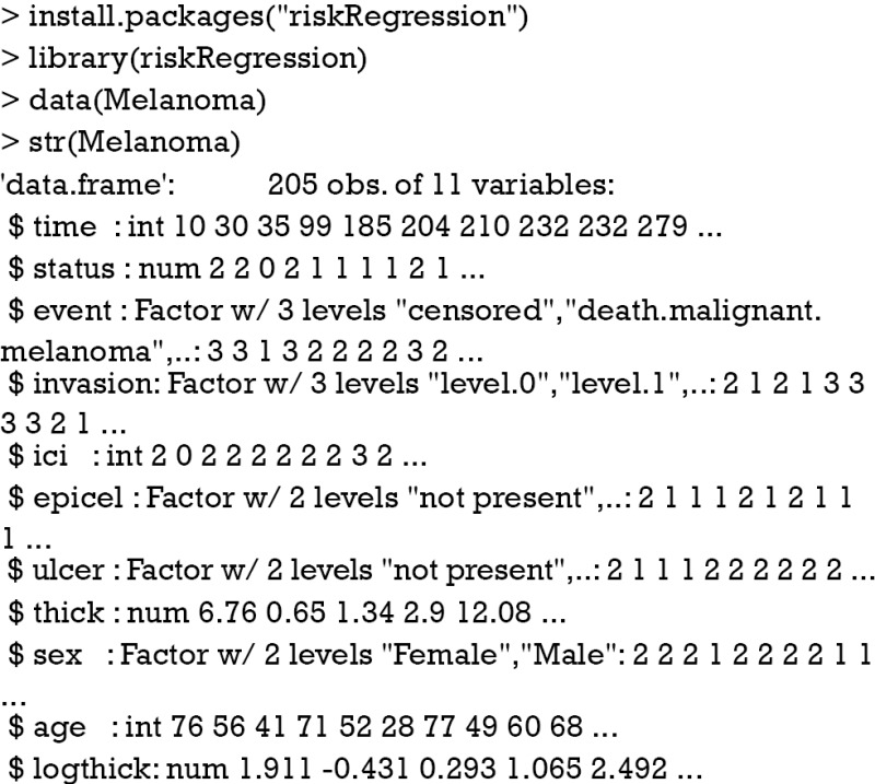
There are 11 variables. The time (time) was measured in days from operation. Status assumes numeric values with 0= censored; 1= died from melanoma and 2= died from other causes. Event is in accordance with status but is converted to a factor variable with three levels. Other variables are risk factors under investigation including invasion, inflammatory cell infiltration (ici), ulcer, thick, sex, age and tumor thickness on log scale (logthick).

Non-parametric comparison of CIFs

CIFs for different causes of failure can be employed for statistical description of survival data with competing risks. This task can be done with Kaplan-Meier (KM) estimator in situations without competing risks. However, the KM method may give biased estimates because it takes the competing risk events as censored. Thus, CIFs for different causes of failure provide additional insights into the survival data at hand. The cuminc() function shipped with the cmprsk package can estimate the CIFs for different causes of failure and allows comparisons between groups.

The arguments specifying an CIF in cuminc() is similar to that in crr() function. The first argument is a failure time variable, and the second one takes a variable with distinct code for different causes of failure. The group argument takes a variable specifying distinct groups. In the example, patients were divided into groups by sex. The estimated CIFs can be visualized with generic function plot(). Figure 1 shows that male patients have higher risk of death from melanoma and other causes than the female. The difference appears larger for failure from melanoma versus failure from other causes. To perform formal statistical test for the difference between groups, modified χ² statistic can be used (10).

Figure 1.

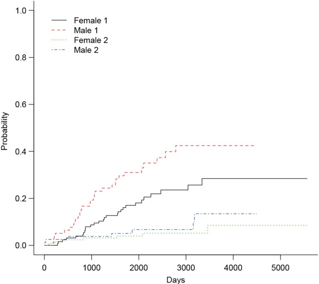
Non-parametric estimates of cumulative incidence functions for deaths from melanoma (status==1) and other causes (status==2). Each outcome is compared between male and female patients.

The first column of the output shows χ² statistic for between-group test, and the second column shows the respective P values. Male patients are more likely to die from melanoma than the female (P=0.016), but there is no significant difference in mortality risk from other causes for male versus female patients (P=0.36).

Cause-specific hazard regression

Cause-specific hazard regression model can be fit with Cox regression by treating failures from the cause of interest as events and failure from other causes as censored observation. The effect of covariates on cause-specific hazard can be estimated with COX proportional hazard regression. The model is fit with coxph() function in the survival package.

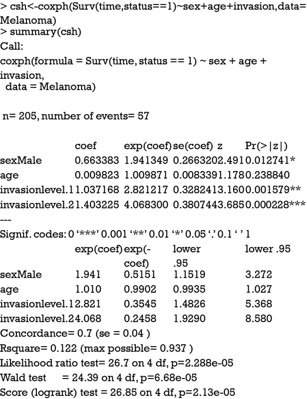
The first argument of the coxph() function takes an object of class Surv, where the “status==1” indicates that only status value of 1 is considered as event and other values are considered as censored. The summary output shows the coefficients and corresponding HR. The last five lines display statistics for the fitness of the model. Detailed interpretation of these statistics can be found in my previous tutorial paper.

Alternatively, the task can be performed using CSC() function contained in the riskRegression package.

The summary output is quite similar to that produced by coxph() function except that CSC() function automatically produces cause-specific hazard models for both types of events (cause 1 and 2). With the fitted regression model, one can predict individual risk with given covariates. For example, I want to predict the risk of a male patient aged 50 years old and has invasion level 2.

The output shows that the cumulative incidences of death from melanoma at time points of 1,000, 2,000, 3,000 days are 0.31, 0.53 and 0.67, respectively.

Subdistribution hazards (SHs) model

SHs model is also known as Fine-Gray model. It is a Cox proportional regression model but the cumulative incidence is associated with SHs. The motivation for Fine-Gray model is that the effect of a covariate on cause-specific hazard function may be quite different from that on CIF. In other words, a covariate may have strong influence on cause-specific hazard function, but have no effect on CIF (9). The difference between cause-specific hazard and subdistribution is that the competing risk events are treated differently. The former considers competing risk events as non-informative censoring, whereas the latter takes into account the informative censoring nature of the competing risk events (1).

The Fine-Gray model can be fit using FGR() function shipped with riskRegression package. This function calls another function crr() from the cmprsk package.

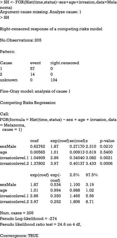
As you can see, the estimated coefficient for cause 1 deviates a little from that obtained from cause-specific hazard model (HR: 1.87 vs. 1.94), reflecting different assumptions for the competing risks. The numerical values derived from Fine-Gray model have no simple interpretation, but it reflects the ordering of cumulative incidence curves (7,9). The cause-specific hazard is the rate of cause 1 failure per time unit for patients who are still alive. However, the cause 1 SH is the rate of cause 1 failure per time unit for patients who are either alive or have already failed from cause 2. In other words, patients who fail from other causes are still in the risk set (8).

The Fine-Gray model can be fit with the crr() function in the cmprsk package. The function arguments are different from that in FGR() function. Although the use of model formula is not supported, the model.matrix function can be used to generate suitable matrices of covariates from factors.

Model prediction

The fitted Fine-Gray model can be used to predict new observations with given combinations of covariates. In the following example, a new dataset containing three patients are given. Covariates of age, sex and invasion levels are defined for them.

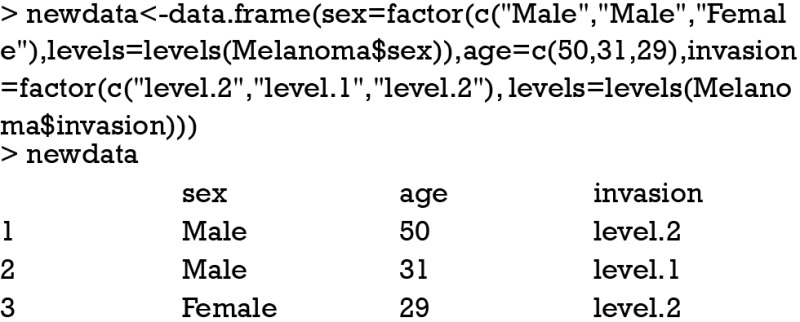
Characteristics of these three patients are displayed in the above output. The data frame need to be transformed to matrix and factor variables be transformed to dummy variables. The predict() function applied to crr object requires the columns of cov be in line with that in the original call to crr() function. Because both sex and invasion are factor variables, they need to be transformed to dummy variables with model.matrix() function. Alternatively, a custom-made function named factor2ind() written by Scrucca and colleagues can be useful (11).

The above output is exactly what we want. Variable sex was coded 1 for male and 0 for female. Invasion was transformed to two 0/1 variables. Age is a continuous variable and remains unchanged.

An object of crr class is passed to the predict() function, followed by a matrix containing covariate combinations. The predict() function returns a matrix (not shown) with the unique cause =1 failure times in the first column, and the other columns giving the estimated subdistribution function corresponding to the covariate combinations at each failure time. The generic function plot() can be applied to draw CIF for each observation (Figure 2).

Figure 2.

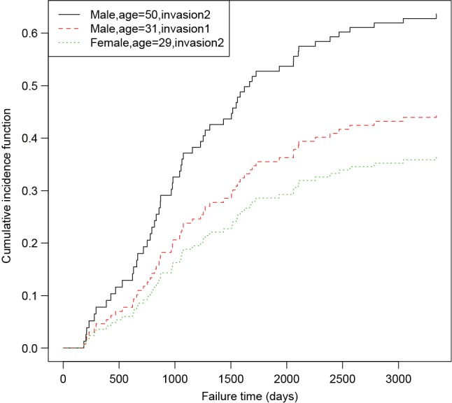
Parametric estimates of cumulative incidence functions for three patients with given covariate values.

The prediction and plotting are more convenient using functions in riskRegression package. The function riskRegression() provides a variety of link functions for survival regression model in the presence of competing risks (12).

The above graphical output gives CIF for patients with characteristics specified in the newdata. The link argument controls the link function to be used: “prop” for the Fine-Gray regression model, “relative” for the absolute risk regression model, and “logistic” for the logistic risk regression model.

Model diagnostic

An important assumption of Cox regression model is the proportionality, which assumes the subdistribution with covariates z is a constant shift on the complementary log-log scale from a baseline subdistribution function. The curves will not cross with each other. Model checking may initially be performed by graphical examination of CIFs.

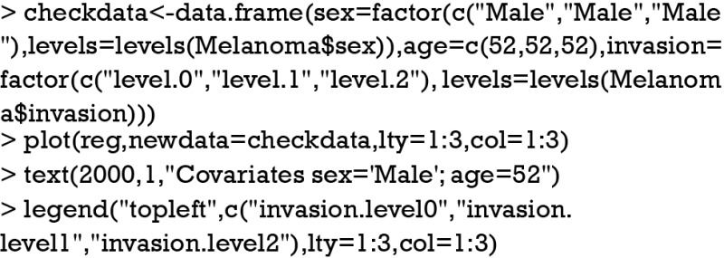
Figure 3 shows the CIFs at different invasion levels, setting age to 52 years and sex to male. There is no evidence of violation to the proportionality assumption for the variable invasion. Another method to check for proportional assumption is to include time dependent covariate in the regression model.

Figure 3.

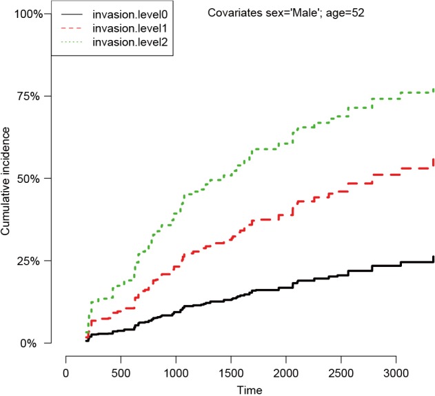
Cumulative incidence functions at different invasion levels, setting age to 52 years and sex to male. There is no evidence of violation to the proportionality assumption for the variable invasion.

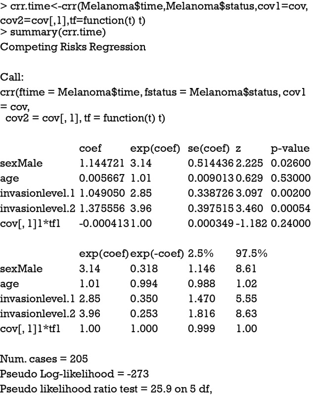
The argument cov2 takes a matrix of covariates that will be multiplied by time. The functions of time are specified in the tf argument. The function takes a vector of times as an argument and returns a matrix. The jth column of the time matrix will be multiplied by the jth column of cov2. For example, a model of the form can be specified in crr() function by (cov1 = x₁, cov2=cbind(x_1,x₁), tf=function(t) cbind(t,t^2)). In the summary output of the Fine-Gray model with time-varying covariate, the last term shows no statistical significance (P=0.24), indicating the effect of sex is time-constant. The riskRegression provides a simple resolution to model time-varying covariate.

Figure 4 shows the time-dependent effects in Fine-Gray regression model for mortality. The curve and corresponding 95% confidence interval are drawn with non-parametric method. It appears that coefficients for level 2 vs. 1 are larger during time period from 0 to 1,000 than that in other times, indicating some slight time interactions (12). However, formal statistical test is not allowed in this setting.

Figure 4.

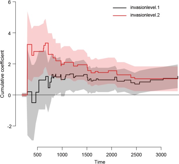
Time-dependent effects in the Fine-Gray regression model for invasion. The nonparametric estimates are shown with 95% pointwise confidence intervals.

The third method for model checking employs Schoenfeld residuals.

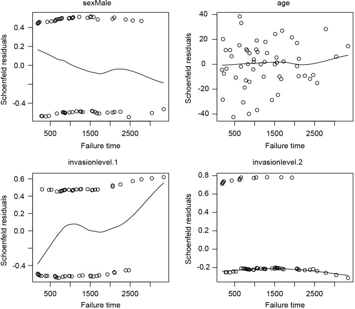
I plot the Schoenfeld residuals against failure time for each covariate. If the proportional assumption is true, the residual should have a constant mean across time. A scatterplot smoother is added for each covariate to check for the assumption (Figure 5). It appears that the invasion level 1 has non-constant residuals across time, indicating a potential violation to the proportional assumption. To formally check the assumption for invasion level 1, we can add an interaction term with time.

Figure 5.

Schoenfeld residuals against failure time for each covariate. It is noted that the residuals follows a non-constant distribution across failure times, indicating a potential violation to the proportional assumption.

The model includes an interaction term with linear time function, which shows that the interaction term (time*invasion level1) is statistically significant (P=0.033).

Biography

Author’s introduction: Dr. Zhongheng Zhang is a fellow physician working at Sir Run Run Shaw Hospital. He graduated from School of Medicine, Zhejiang University in 2009, receiving Master Degree. His major research interests include hemodynamic monitoring in sepsis and septic shock, delirium, and outcome study for critically ill patients. He is experienced in data management and statistical analysis by using R and STATA, big data exploration, systematic review and meta-analysis. He has published more than 50 academic papers (science citation indexed) that have been cited for over 700 times. He has been appointed as reviewer for 10 journals, including Journal of Cardiovascular Medicine, Hemodialysis International, Journal of Translational Medicine, Critical Care, International Journal of Clinical Practice, Journal of Critical Care.

References

- 1.Satagopan JM, Ben-Porat L, Berwick M, et al. A note on competing risks in survival data analysis. Br J Cancer 2004;91:1229-35. 10.1038/sj.bjc.6602102 [DOI] [PMC free article] [PubMed] [Google Scholar]
- 2.Latouche A, Allignol A, Beyersmann J, et al. A competing risks analysis should report results on all cause-specific hazards and cumulative incidence functions. J Clin Epidemiol 2013;66:648-53. 10.1016/j.jclinepi.2012.09.017 [DOI] [PubMed] [Google Scholar]
- 3.Bakoyannis G, Touloumi G. Practical methods for competing risks data: a review. Stat Methods Med Res 2012;21:257-72. 10.1177/0962280210394479 [DOI] [PubMed] [Google Scholar]
- 4.Haller B, Schmidt G, Ulm K. Applying competing risks regression models: an overview. Lifetime Data Anal 2013;19:33-58. 10.1007/s10985-012-9230-8 [DOI] [PubMed] [Google Scholar]
- 5.Schallom ME, Prentice D, Sona C, et al. Heparin or 0.9% sodium chloride to maintain central venous catheter patency: a randomized trial. Crit Care Med 2012;40:1820-6. 10.1097/CCM.0b013e31824e11b4 [DOI] [PubMed] [Google Scholar]
- 6.Zhang Z, Pan L, Ni H. Lumen nonpatency in the presence of competing risks. Crit Care Med 2012;40:3108; author reply 3108-9. 10.1097/CCM.0b013e31826324e8 [DOI] [PubMed] [Google Scholar]
- 7.Andersen PK, Keiding N. Interpretability and importance of functionals in competing risks and multistate models. Stat Med 2012;31:1074-88. 10.1002/sim.4385 [DOI] [PubMed] [Google Scholar]
- 8.Andersen PK, Geskus RB, de Witte T, et al. Competing risks in epidemiology: possibilities and pitfalls. Int J Epidemiol 2012;41:861-70. 10.1093/ije/dyr213 [DOI] [PMC free article] [PubMed] [Google Scholar]
- 9.Fine JP, Gray RJ. A proportional hazards model for the subdistribution of a competing risk. J Am Stat Assoc 1999;94:496-509. 10.1080/01621459.1999.10474144 [DOI] [Google Scholar]
- 10.Gray RJ. A class of K-sample tests for comparing the cumulative incidence of a competing risk. Ann Stat 1988;16:1141-54. 10.1214/aos/1176350951 [DOI] [Google Scholar]
- 11.Scrucca L, Santucci A, Aversa F. Regression modeling of competing risk using R: an in depth guide for clinicians. Bone Marrow Transplant 2010;45:1388-95. 10.1038/bmt.2009.359 [DOI] [PubMed] [Google Scholar]
- 12.Gerds TA, Scheike TH, Andersen PK. Absolute risk regression for competing risks: interpretation, link functions, and prediction. Stat Med 2012;31:3921-30. 10.1002/sim.5459 [DOI] [PMC free article] [PubMed] [Google Scholar]