Nano Random Forests to mine protein complexes and their relationships in quantitative proteomics data

Nano Random Forests is a machine learning-based approach to extract valuable information about multiprotein complexes in collections of proteomics experiments. In mitotic chromosome data, it retrieves known relationships among kinetochore substructures and provides highly specific predictions about uncharacterized protein function.

Abstract

Ever-increasing numbers of quantitative proteomics data sets constitute an underexploited resource for investigating protein function. Multiprotein complexes often follow consistent trends in these experiments, which could provide insights about their biology. Yet, as more experiments are considered, a complex’s signature may become conditional and less identifiable. Previously we successfully distinguished the general proteomic signature of genuine chromosomal proteins from hitchhikers using the Random Forests (RF) machine learning algorithm. Here we test whether small protein complexes can define distinguishable signatures of their own, despite the assumption that machine learning needs large training sets. We show, with simulated and real proteomics data, that RF can detect small protein complexes and relationships between them. We identify several complexes in quantitative proteomics results of wild-type and knockout mitotic chromosomes. Other proteins covary strongly with these complexes, suggesting novel functional links for later study. Integrating the RF analysis for several complexes reveals known interdependences among kinetochore subunits and a novel dependence between the inner kinetochore and condensin. Ribosomal proteins, although identified, remained independent of kinetochore subcomplexes. Together these results show that this complex-oriented RF (NanoRF) approach can integrate proteomics data to uncover subtle protein relationships. Our NanoRF pipeline is available online.

INTRODUCTION

Proteins influence many processes in cells, often affecting the synthesis, degradation, and physicochemical state of other proteins. One strategy that diversifies and strengthens protein functions is the formation of multiprotein complexes. For this reason, identification of partners in complexes is a powerful first step to studying protein function. However, determination of membership to or interaction with protein complexes remains an arduous task, mainly achieved via demanding biochemical experimentation. The latter can be limited by the ability to overexpress, purify, tag, stabilize, and obtain specific antibodies for the proteins in complexes of interest. Thus any methods that facilitate protein complex identification and monitoring (Gingras et al., 2007; Kustatscher et al., 2014; Skinner et al., 2016) have the potential to accelerate the understanding of biological functions and phenotype. The vast amount of proteomics data already available represents a largely untapped resource that could potentially reveal features undisclosed by traditional analysis, such as condition-dependent links, intercomplex contacts, and transient interactions.

Biochemical cofractionation has been widely used to identify protein complexes. Members of a multiprotein complex typically coelute with a single mass, charge, elution rate, and so on in techniques such as chromatography, gel electrophoresis, and coimmunoprecipitation. Another common way to discover complexes is to combine chemical cross-linking, fractionation, and mass spectrometry, which covalently fixes proteins that interact (Leitner et al., 2016). However, biochemical fractions often contain contaminants, that is, proteins that are not genuine subunits of the complex of interest, despite having similar biochemical properties. One way to reveal bona fide members is to combine several fractionation experiments, as well as perturbations (Moore and Lee, 1960). Members of a complex will behave coordinately, whereas contaminants will usually show a more independent behavior. From a quantitative perspective, this translates into protein covariance—the covariance of proteins within a complex is stronger than that with contaminants. As additional biochemical fractionation conditions are considered, high covariance sets true members of a complex apart from contaminants or hitchhikers. This principle was used recently in a large-scale effort that predicted 622 putative protein complexes in human cells by assessing the coordinated behavior of proteins across several fractionation methods, among others (Havugimana et al., 2012; Michaud et al., 2012).

Covariance among members of protein complexes has been observed in several integrative proteomics experiments (Ohta et al., 2010; Borner et al., 2014) and even used to predict association with complexes (Andersen et al., 2003; Borner et al., 2014). This relies on the fact that the cofractionation of proteins that are functionally interconnected will be affected by common parameters, such as knockouts or varying biochemical purification conditions. However, performing covariance analysis using multiple quantitative proteomics data sets is nontrivial. First, experimental or biological noise hampers quantitation of protein levels. Second, only a fraction of the experiments may be informative for any given complex. Third, proteins may go undetected, leading to missing values. Fourth, the relationship between different protein groups may only be observed under specific circumstances. The power of multivariate analysis methods such as principal component analysis (PCA) and hierarchical clustering or k-nearest neighbors (KNN) could be limited when a protein complex’s signal in the data is affected in all these ways. Here we show that the supervised machine learning technique Random Forests can overcome these limitations, distinguish the covariance of small protein groups, and provide biologically sound, predictive insights into protein complex composition, relationships, and function. We describe this approach using as an example the behavior of multiprotein complexes in mitotic chromosomes.

RESULTS

Random Forests can detect small protein complexes in simulated organelle proteomics data

Proteins in multiprotein complexes have been shown to covary across quantitative proteomics experiments of organelles (Ohta et al., 2010; Borner et al., 2014). That is, the absolute or relative quantities of proteins that together form a complex increase or decrease in a coordinate manner. This concerted behavior forms a potentially detectable “signature” of the complex across sets of proteomics experiments. Other proteins that share the same signature may be functionally related to the complex.

We wondered how strong a complex’s signature would need to be for its detection. The signature is an outcome of the resemblance of each protein’s behavior to that of each other and how much the group stands out from other groups. We reasoned that the strength of the signature could be modulated in two ways: 1) by controlling the fraction of informative experiments (experiment subsets in which the members of the complex correlate) and 2) by different amounts of noise. Less informative experiments should “dilute” the complex’s signal, whereas stronger noise should lead to fluctuations away from the common behavior. We therefore constructed artificial proteomics data in which we could independently control these two properties and evaluate their influence on detecting a hypothetical complex.

We generated artificial proteomics tables (Figure 1A) by populating random values into tables of similar sizes to our original data set: 20 “experiment” columns by 5000 “protein” rows. In those tables, 12 “proteins,” which were intended to represent a hypothetical protein complex, were constrained to have identical behavior in a fraction X of columns while leaving independent random values in the remaining experiments. This action imitated situations in which a complex covaried in only an informative subset of experiments (Figure 1A, middle). For example, if X = 0.5, 10 of 20 “experiments” would contain the signature behavior. Next we jittered all the entries in the table by adding Gaussian noise of strength Y. Figure 1B illustrates the data generated by this approach and exemplifies visually how the number of informative variables and noise contribute to a protein group’s signature behavior.

FIGURE 1:

Supervised machine learning algorithm RF can detect small, correlated protein groups in artificial proteomics data. (A) Depiction of the procedure used to simulate proteomics data with “protein” rows and “experiment” columns. Some rows are made identical (red tones) in a fraction of experiments to simulate a hypothetical complex (HC) that correlates in some experiments, and Gaussian noise is then added elementwise to each table entry. (B) Visual description of a hypothetical complex (red) vs. other randomly generated proteins (gray) as the number of experiments (left–right) and the noise (bottom-up) affect the protein values in the experiments. (C) Visualization of the output from RF. The RF score denotes how much a protein resembles the complex, and separation quality indicates how easily unrelated proteins covary with the complex. Red and gray dots depict the hypothetical complex and other proteins, respectively. (D–F) Heat maps showing how the fraction of informative experiments (x-axis) and the noise amount (y-axis) affect the mean correlation (D), RF score (E), and separation quality (F) of proteins in a complex. In each square, the value projected is the mean of means of five independent groups.

We wondered first whether the mean of pairwise correlations between proteins of a complex would suffice to reveal membership as levels of noise and informative experiments changed. As one would expect, when the noise was low and the fraction of informative experiments was high, protein correlation was high. However, it dropped rapidly with slightly weaker signatures (Figure 1D).

We then asked whether the machine learning algorithm Random Forests (RF; Breiman, 2001) would recognize stronger or weaker signatures in the behavior of the hypothetical complex (for an introductory explanation of the algorithm, see Materials and Methods). RF has been used in several biological data contexts, including gene expression, protein–protein interactions, and mass spectrometry (Fusaro et al., 2009; Qi, 2012). Specifically, we asked whether RF could distinguish our hypothetical complex (i.e., the positive class) from an independent group of other proteins (i.e., the negative class) composed of 365 rows in the random protein table (Figure 1A, middle). In two previous studies from our group (Ohta et al., 2010; Kustatscher et al., 2014), we used RF because 1) it samples combinations of experiments and attempts to draw a boundary between a positive and a negative class, 2) it is nonparametric and can handle missing values (Qi, 2012), and 3) for every “protein,” an RF score between 0 and 1 indicates whether it behaves as part of the hypothetical complex (Figure 1C). Proteins that are part of the positive and negative classes also obtain an unbiased score regardless of whether they belong to the training classes (see Materials and Methods).

Figure 1E shows that the RF score of the hypothetical complex remained high even with few informative experiments but fell significantly with higher noise. Therefore, if one looked at the RF score alone, even small amounts of noise could lead to failure to recognize members of the true complex (false negatives), even when they initially had a fairly strong correlation. These results suggest that on its own, the RF score is not robust to noisy conditions even when correlation in a complex is high.

We reasoned that a noise-induced decrease in RF scores could be tolerated as long as the scores of members of the hypothetical complex were overall higher than those of the negative class. On the other hand, levels of noise too high and too few informative experiments could lead to false positives. To strike a balance, we searched for an RF score that, if used as a boundary between the two classes, maximized separation quality, that is, made the fewest class misassignments between the hypothetical complex and the hypothetical contaminants. This can be assessed by the Matthews correlation coefficient (MCC; exemplified in Figure 2A, bottom). Figure 1F shows that class separation quality remains high for different levels of noise and small fractions of informative experiments. All measures showed the lowest values for the weakest signatures, where the complex can no longer be distinguished from randomly covarying groups. Taking the results together, we conclude that RF is able to distinguish significant signatures of a protein group under conditions of high noise and few informative experiments, even though the group could be as small as a protein complex. Because of the small training set size, we refer to this instance of Random Forests as NanoRF.

FIGURE 2:

RF can detect small protein complexes in chicken chromosome SILAC proteomics experiments. Red, protein complex; blue, contaminants/hitchhikers; orange, proteins showing high covariance with identifiable members of the complex (RF scores as high as those of the complex) that potentially associate with it. (A) Logic of the procedure to detect complexes with RF. Groups separable in multiple dimensions (only two depicted) yield a higher MCC than inseparable groups. (B) RF scores of multiple complexes vs. the same set of contaminants/hitchhikers and randomly selected groups from the table. Bottom, randomly chosen sets of proteins yields poor red/blue separation, implying that the members of the mock complex are unidentifiable. In this case, the next optimal cut-off is driven by exclusion of contaminants. (C) ROC performance curves of the RF as a classifier for each protein complex and for two randomly selected protein groups (gray, black). Diagonal shows the random assignment scenario. (D) Kernel densities of MCC values for 500 RF runs of each complex and 5000 runs for randomly assigned groups (black). Sample sizes: 10 for positive class and 425 for negative class. All distributions were made of height 1 for visualization purposes.

RF analysis can distinguish protein complexes from contaminants in proteomics experiments of mitotic chromosomes

Our group has collected and published stable isotope labeling by amino acids in cell culture (SILAC) proteomics data of mitotic chromosomes isolated from chicken DT40 wild-type and knockout cell lines (Ohta et al., 2010, 2016). The proteins targeted for knockouts belong to a range of mitotic chromosome complexes of two groups: structural maintenance of chromosomes (SMC) complexes such as condensin (SMC2-4), cohesin (SMC1-3; Uhlmann et al., 1999; Sonoda et al., 2001; Mehta et al., 2012), SMC5-6 (Stephan et al., 2011; Wu and Yu, 2012), and the kinetochore (Ska3). We previously used RF to distinguish between large groups of “true” chromosomal proteins and potential hitchhikers or contaminants. Given that RF could distinguish small covarying groups in simulated data, we asked whether it could detect known small protein complexes based on real data and whether any other proteins shared the signature of the complexes.

Figure 2A illustrates our strategy to detect protein complexes in mitotic chromosomes and retrieve proteins that may be functionally linked with them. First, we choose a protein complex (Figure 2, red dots) and a set of curated hitchhikers (Figure 2, blue dots; Ohta et al., 2010), which serve as the negative class (Supplemental Table S2). Then we use RF to distinguish the complex from the hitchhikers on the basis of our proteomics data. Every protein gets an RF score, and we look for a boundary cut-off that maximizes class separation quality, that is, such that most members of a complex are above it and most contaminants are below. True members that exceed the cut-off are said to be “identifiable.” Other, nonmember, noncontaminant proteins above that cut-off together with true members are said to covary/associate with them (Figure 2, A and B, orange dots). To find the boundary cut-off and its significance, we use the MCC (Figure 2A, bottom) as in the previous section. A more traditional way to evaluate the significance of this result is to consider a hypergeometric test. If we were to draw proteins at random from a bag in which true members and hitchhikers were mixed, such a draw would be analogous to setting an RF cut-off. For a given draw, the larger the number of true members and the lower the number of hitchhikers, the lower is the probability of such draw.

We analyzed a number of different complexes with RF (Figure 2B). In particular, we performed NanoRF on the constitutive centromere–associated network (CCAN), the KNL-Mis12-Ndc80 (KMN) complex, nucleoporin 107-160 (Nup107-160)/RanGAP, SMC 5/6, cohesin, and ribosomal proteins. Figure 2B shows an overview of the RF result for each complex. Most complexes yielded a high separation quality, and most bona fide subunits were assigned higher RF scores than the contaminants. Other proteins (orange) distinguished themselves from hitchhikers, with scores as high as bona fide complex subunits. These significantly covarying proteins likely correspond to a mix of known, putative, and potentially spurious associations, which we attempt to dissect in the following sections. Supplemental Table S2 gives the full list of proteins associated with each complex.

A common concern in supervised machine learning is overfitting—a situation in which the algorithm performs well for reasons other than the inherent properties of proteins in the data. This can be due, for example, to training set bias. A way to control for the latter is through out-of-bag (OOB) analysis, which overlaps functionally with cross-validation. For every tree constructed, the algorithm leaves a random number of training observations out. This internally avoids biasing the training toward particular observations (Breiman, 2001). Because we built our trees in this way, the results shown are already controlled for training set bias.

An algorithm capable of overfitting may be able to identify any arbitrary group of proteins by leveraging noise and other irrelevant properties. Therefore, to further rule out overfitting, we ran RF on 5000 protein sets generated at random from our data set. The size of those test sets (10 random positive-class proteins and 400 random negative-class proteins) was in the range of the chromosomal protein complexes we investigated, which ranged between seven and 20.

Figure 2B, bottom, shows the result of performing RF on a randomly picked target group of proteins rather than a complex and another randomly picked group as a mock group of contaminants/hitchhikers. Both classes intercalate; in other words, RF classification shows poor performance (there is no evidence for any discrete group in the data), and no member of the mock target group is identifiable (RF score close to zero). Because the RF classification and MCC values are of such poor quality, interpretation of the RF is undefined in these conditions. Our results with the random groups contrast starkly with the successful identification of proteins separating as protein complexes from the negative class (Figure 2B, top).

We further evaluated the significance of our results using receiver-operating characteristic (ROC) curves (Figure 2C) and MCC values (Figure 2D). Starting from the highest RF score, an ROC curve evaluates the fraction of positive class members recovered (true positives) on the vertical axis versus the negative class members recovered (false positives) on the horizontal axis. An ROC curve that climbs vertically is favorable because it means that the RF score is sensitive to the complex. Under these circumstances, the area under the ROC curve (AUC) is >0.5. In contrast, if the RF score contains a poor signal, the positive and negative classes are retrieved randomly. In this case, the ROC curve climbs up the diagonal and has an area of ∼0.5. In our analysis, all of the complex-specific RF retrieved ∼70% of the complexes before any false positives were collected (Figure 2C). All our complexes showed an AUC between 0.9 and 0.999 (Supplemental Table S2), implying accurate classification. In contrast, ROC curves of the randomly selected groups (examples in Figure 2C, black and gray lines) remained close to the diagonal.

Finally, for some complexes we studied, it could be a matter of chance that they separated well from the negative class. We sought to address how likely it is for a random group to obtain a high separation quality by chance in our data set. We evaluated the distributions of class separation quality (as quantified by the peak MCC values) for real complexes and for randomly sampled protein groups (Figure 2D). The highest MCC value obtained for the random classes was 0.543 (p ≈ 0.0002, N = 5000), and the minimum MCC value for the complex separation was 0.71 (p ≈ 0.002, N = 500). These results support the hypothesis that the NanoRF can distinguish between protein complexes and contaminants in real data.

Integration of several complex-specific RF results reveals known and novel interdependences among protein complexes

The covariance of each complex could be its unique signature or could overlap with that of other complexes, possibly implying conditional interdependence among complexes. We decided to test this hypothesis with kinetochore subcomplexes because there is significant contact among them. To this aim, we analyzed two-­dimensional (2D) plots of RF for different complexes (Figure 3).

FIGURE 3:

Known and novel interdependences among complexes revealed by RF. Highest separation quality thresholds are depicted by dashed lines. (A) A 2D diagram to visualize intersections between RF results for different complexes. Proteins above both thresholds (pink quadrant) associate with both complexes, whereas those above only one remain independent. (B) Possible scenarios of interdependence between complexes inferred from 2D RF plots. A hierarchical effect (bottom left) occurs when the RF of one complex (squares) brings up the other complex (triangles) but not vice versa. A third-group link (bottom right) is equivalent to a double hierarchical effect on the pink circle complex. Many three-group relationships exist; in the case shown, the circle complex is the only link between the triangle and square complexes. (C, D) A 2D interdependence plot of the CCAN (C and D, squares) vs. the Nup107-160/RanGap complex (C, triangles) and the SMC 5/6 complex (D, triangles).

We categorized several possible interdependence scenarios between kinetochore complexes (Figure 3, A and B). According to these scenarios, the CCAN and the Nup107-160/RanGAP complex (Figure 3C) appeared to be independent, that is, they do not associate with each other. In contrast, the KMN network associated with both. We concluded that perturbations on both CCAN and Nup107-160 have a hierarchical effect on KMN (i.e., their effects propagate to KMN but not vice versa), implying that the latter is involved in links between inner and outer kinetochore. These observations are consistent with current models of the kinetochore (Kwon et al., 2007; Screpanti et al., 2011). Supplemental Figure S1 shows other proteins associated with the CCAN, Nup-Ran, or SMC5-6 complexes.

Even though the CCAN RF prediction was rich in associated proteins, which might be expected from a crowded chromatin environment, the entire condensin complex associated with the CCAN. This dependence might imply a potential relationship between these complexes that merits further study. Finally, Figure 3D shows that the CCAN RF prediction is independent of the SMC 5/6 complex, and no CCAN protein cofractionated with ribosomal proteins (Supplemental Figure S2). Together these results show that, by integrating the outcome of several complex-specific RF results, we can reconstruct known dependences at the kinetochore and identify novel intercomplex dependences. Of note, none of these relationships was directly addressed a priori by the experiments used.

We suggest that this strategy to infer protein functions and relationships by training RF with small protein complexes be named NanoRF. The results presented here constitute a proof-of-concept demonstration of the method in the context of the kinetochore. A thorough use in the context of SMC complexes, as well as experimental verification of NanoRF predictions, can be found in Ohta et al. (2016). Our code, as well as a step-by-step guide on how to perform NanoRF, is available (Montano-Gutierrez, 2016).

DISCUSSION

A recurrent goal in the postgenomic era has been to make sense of increasing amounts of underexploited data, including noisy and incomplete proteomics output. Our results show that, even with high noise and when few experiments are informative, small groups of strongly covarying proteins, that is, multiprotein complexes, can be recognized by their coordinated behavior using RF (Figures 1 and 2). In data of this type, statistical measures such as the mean correlation (Figure 1C) or absolute RF score of members in a complex can drop considerably (Figure 1D). We demonstrated that lower RF scores can be informative as long as complexes separate out from contaminants by their RF score (Figure 1F). By tolerating a decrease of the RF score while maximizing separation quality, we were able to predict highly specific associations with complexes (Figure 2B) and retrieve known intercomplex relationships in our data set (Figure 3). Because no experiment targeted all of the complexes detected, this strategy could potentially identify protein function in any combination of comparable proteomics results.

In simple terms, NanoRF attempts to find the strongest possible signature for a complex (if any exists) within a specific data set. The premise is that any other protein whose RF score is as high as that of bona fide members while being clearly distinguishable from contaminants is essentially difficult to distinguish from the complex itself. Our results with real complexes suggest that the strongest statistical associations we found have biological relevance.

Comparison between NanoRF and other methods

Two previous studies from our group used RF to attempt to find general trends shared by functional members of chromosomes (Ohta et al., 2016) or interphase chromatin (Kutstatscher et al., 2014) in proteomics data. The evidence presented in the present work suggests that the “true chromosome class” is the integration of the signatures of multiple protein complexes covarying in specific, distinguishable ways. Because of strong yet conditional, complex-specific covariance, adding more than one complex to a training class may restrict the performance of RF. Compared to multiclassifier combinatorial proteomics and fractionation profiling (Borner et al., 2014), our prediction would upgrade, for example, from “true chromosomal protein” to “protein dependent on complex A but not complex B.” To cite another example, the polybromo- and-BAF-containing (PBAF) complex (ARID2, PBRM1, BRD7, SMARCB1 and SMARCE1) associated specifically with Nup107-160 but not with the CCAN (Supplemental Figure S1A). Consistent with this prediction, another bromodomain-containing protein, CREBBP, was found to interact with Nup98 in the Nup107-160 complex and was linked to Nup98 oncogenicity (Kasper et al., 1999).

Methods such as fractionation profiling (FP; Borner et al., 2014) and multivariate proteomic profiling (Borner et al., 2012) are based on the use of guilt-by-association analyses to similarly detect protein complexes and cleverly deal with the intricate nature of proteomics data, in particular, missing values, but do not account for the conditional covariance of the complex, that is, a signal being present in only a few experiments. We showed that NanoRF finds such covariance even when there is significant noise. It successfully predicted proteins with previously uncharacterized links to mitosis (Ohta et al., 2016).

NanoRF is a supervised method that is ideal for deeply exploring complexes or protein groups that are already of interest to the researcher. Such groups may be either true protein complexes or any potential protein group hypothesized to covary. We demonstrated that known protein complexes show a strong detectable signature, but other kinds of protein groups may be detectable as well. For discovery of protein complexes, other methods, including unsupervised RF or clustering, are more suitable.

Potential pitfalls and statistical considerations of NanoRF

It is not possible to conclude from computational analysis alone that the relationships predicted by NanoRF are direct physical interactions between the aforementioned protein complexes. Nevertheless, our results come strictly from protein-level dependences (or indirect effects of these) rather than changing expression levels, and so physical associations are likely. Further support for this comes from a study in which we used the algorithm to explore chromosome structure. NanoRF associated VRK1 and PTPN6 with CCAN and RZZ, respectively. Fluorescence microscopy showed localization of VRK1 to chromosomes and PTPN6 to microtubules (Ohta et al., 2016).

We believe that finding the objectively best separation quality lessens the burden to select an arbitrary significance cut-off for candidates, especially as more uninformative experiments are collected. We intentionally avoided using a hypergeometric p value as a significance measure because 1) the exact p values for all of our complexes are ≤10⁻¹¹ (Supplemental Table S2), 2) p values were strongly influenced by the number of proteins in the complex, and 3) they were undefined for some of the random group RF results in which neither of the two classes was above the MCC threshold (Figure 2B, bottom).

Instead of direct p value use, the significance of the predictions by NanoRF is subject to the probability of obtaining a high separation quality by chance for a given data set. To minimize the risk of type I error, we suggest that the peak MCC for a complex at the cut-off should be higher and nonoverlapping with the MCCs obtained for randomly assigned protein groups in a data set. In our analysis, the probability of obtaining an MCC as high as that of real complexes by chance was negligible—our sampled MCC distributions did not overlap (Figure 2D)—but it might vary for other data sets. Naturally, a lower MCC might be accepted at the risk of more false positives.

For prediction of associations with a complex, the false discovery rate for each complex should be proportional to the fraction of negative-class proteins that surpass the classification threshold. A small negative class could lead to underestimating false positives because higher noise might increase the RF score of spurious proteins. Therefore a large negative class might be essential for a realistic false discovery rate estimation (Tarca et al., 2007), and a small one could be compensated with a more stringent prediction cut-off for the RF score.

Potential applications of NanoRF

In the context of all the massive protein–protein interaction networks being identified, we face a lack of detail in the functionality, hierarchy, specificity, and conditionality of these interactions. We sowed that NanoRF could satisfy these unmet needs by providing deep insight into protein complexes.

Experiments are informative if members of a complex covary in them (Figure 1A). Differentiating between informative and noninformative experiments (feature selection) could be a powerful tool for protein complex data mining. For example, a specific set of perturbations might break the stoichiometry (and hence the correlation) in a complex. In this direction, our NanoRF pipeline (Montano-Gutierrez, 2016) includes a calculation of each experiment’s “importance” for classification, although exploiting such importance might not be straightforward. This estimation employs the Gini importance, which compares classification performance with or without a given experiment. A thorough analysis of importance measures is provided by Louppe et al. (2013).

We speculate that NanoRF could be performed on the same complex multiple times, each time using a distinct subset of experiments. These subsets could correspond, for example, to different time points or biological conditions, such as drug treatments. Such analysis could potentially inform how a complex’s identifiability changes with the experiments or whether there is a difference in associated proteins from one condition to the next. Such changes in retrieval might provide insight into conditional binding partners or the biology of specific conditions, drugs, or diseases.

Of importance, NanoRF does not require proteins to remain physically attached to each other during analysis, which may be difficult for weakly interacting or insoluble protein complexes such as those associated in chromatin or membranes.

Here we described NanoRF, which uses supervised machine learning to 1) detect protein complexes of interest in noisy data sets with few informative experiments, 2) predict proteins that have functional associations with specific complexes, and 3) evaluate the relationship between complexes according to their behavior. NanoRF enables hypothesis-driven data analysis from ever-increasing, underexploited quantitative proteomics data. It is generally assumed that machine learning requires large training sets to work. However, we established that RF can retrieve strikingly small protein complexes, their associated proteins, and relationships between complexes from ordinary proteomics results. We anticipate NanoRF to complement experimental cofractionation approaches such as immunoprecipitation.

MATERIALS AND METHODS

Cell culture, mitotic chromosome isolation, and SILAC mass spectrometry

The present analysis was done by collecting and integrating the data from previous work (Ohta et al., 2010, 2016). All cell culture, mitotic chromosome extraction, and mass spectrometric analysis procedures are detailed there. In brief, chromosomes were extracted from wild-type chicken DT40 cells (clone 18), as well as from conditional knockouts for chromosome structure proteins SMC2, CAP-H, CAP-D3, Scc1, and SMC5 (Hudson et al., 2003; Green et al., 2012; Ohta et al., 2016) and a genetic knockout of kinetochore protein Ska3 (Ohta et al., 2016). All strains were incubated with nocodazole for 13 h to arrest the cells in metaphase. In the case of the conditional knockouts, cells were incubated with doxycycline for 20–60 h to inhibit target gene expression before nocodazole treatment. Mitotic chromosomes of wild-type and knockout (KO) cell lines were grown respectively in “heavy” and “light” medium and then mixed in equal amounts judging by Picogreen quantification. In the Ska3 KO experiment, samples were equated using histone H4 as a reference. Thirty trypsin-digested fractions were desalted using StageTips (Rappsilber et al., 2003) and analyzed by liquid chromatography/mass spectrometry (MS) on an LTQ-Orbitrap (Thermo Fisher Scientific) coupled to high-performance liquid chromatography via a nanoelectrospray ion source. MS data were analyzed using MaxQuant 1.0.5.12 for generating peak lists, searching peptides, protein identification (Cox and Mann, 2008), and protein quantification against the UniProt database (release 2013_07).

Preparation of MS data for NanoRF

Only the SILAC ratios from the Protein groups MaxQuant output table were used. As for the Ska3 KO experiment, SILAC ratio column values were taken directly from Ohta et al. (2010) and reindexed according to the rest of the experiments. The ratio columns in Supplemental Table S1 were directly and only used for the analysis. The features included consist only of the SILAC ratio columns of our experiments—no other feature selection, engineering, or combination was performed a priori.

All the raw MS and MaxQuant output data, including those from the Ska3 experiment (Ohta et al., 2010), are available via ProteomeXchange with identifier PXD003588. Missing values were substituted by the median value of each experiment, as is common practice in RF applications. We reasoned that doing so would penalize the lack of observations by giving the same score to missing proteins of both positive and negative classes, which in turn increases the intersection between classes and thereby decreases separation quality.

RF analysis

The analysis was done with a custom R pipeline based on Leo Breiman and Adele Cutler’s RF algorithm (Breiman, 2001) implemented in R (Liaw and Wiener, 2002). All of the scripts used are freely available through a Github repository (Montano-Gutierrez, 2016) and include a step-by-step R guide script to perform NanoRF on any particular data set. The RF algorithm attempts to find a series of requirements in the data that are satisfied by the positive training class and not by the negative training class. All of these decisions are performed sequentially, and hence they become a decision tree. An example of a decision tree would be “proteins with values >x in experiments 1 and 2. Out of those, proteins with values <y in experiments 3 and 5.” Because the best set and decision sequence is not known a priori, the best bet is to generate many decision trees at random (hence the name Random Forest). Each tree votes for all compliant proteins as members of the positive class. The clearer the difference between the two classes in the data, the larger is the number of trees that will vote for the positive class as indeed positive. The RF score (calculated for each protein) is the fraction of trees that voted for a protein as positive. To get a score for the members of the positive class as well, during the generation of each tree, some of the members of the positive and negative classes are left out and treated as unknown. This OOB procedure intrinsically controls for training set bias.

We set the number of trees in the forest to 3000 in each run. The Matthews correlation coefficient was calculated by using the formula

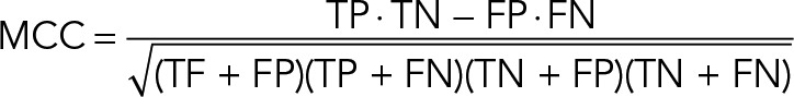where TP indicates true positives, FP false positives, TN true negatives, and FN false negatives. For null values of any of the sums in the denominator, the MCC was defined as 0. To choose a particular RF score as a cut-off, we evaluated 100 possible cut-offs between RF scores 0 and 1 and kept the one that maximized the MCC. For cut-offs with the same maximum MCC, we chose the smallest RF as a cut-off to maximize sensitivity.

Simulation and random protein group size choices

The group size for simulated and randomly chosen protein were chosen to correspond as closely as possible to the values in our original data set. The original data set consists of 4998 protein rows identified in the Maxquant analysis and 12 columns (each corresponding to one of the experiments we used for this analysis). The manually curated data set of hitchhikers and contaminants (Ohta et al., 2010), which we used as the negative class, comprised 367 of the 4998 protein rows. With those actual parameters in mind, we defined the number of rows, columns, and controls as 5000, 20, and 400, respectively, for numerical simplicity.

We expect the trends found in our simulations (although not the specific numbers) to be general to different data set sizes. Of importance, we took care to minimize the number of variables in this analysis that depend on data set size. In particular, 1) we study the proportion (rather than raw number) of informative variables in the data set, 2) the results in Figure 1, D–F, are the mean of give independent hypothetical complexes in order to yield robust results, and 3) the simulated experiments were standard normal distributions, which should yield convergent results with larger numbers.

In-silico analysis of noise and informative experiment fraction

We arbitrarily generated matrices with ∼5000 “protein” rows and 20 “experiment” columns (sizes similar to our SILAC ratio matrix) by sampling a standard normal distribution. In each matrix, 365 “proteins” were selected to be part of the negative class and five groups of 12 proteins were set to be identical within their group in 2,4,…, 20 “experiments” (Figure 1, D–F, horizontal axis). Next all of the values in each matrix were jittered with Gaussian noise with SD of 0.2, 0.4,…, 2 (Figure 1, D–F, vertical axis). Missing values were not added to the simulations, on the basis that they would be filled with median values, which would add variance and thus have similar effect to noise addition. We then ran the RF analysis for the five groups versus the negative set. The values in Figure 1, D–F, are the mean of means of the RF score and of highest MCC for each positive group. The correlation was the mean of intragroup correlations of all positive groups.

Definition of protein group covariance

The covariance between random variables is only defined pairwise, and, as such, the “mean correlation of a complex” as mentioned in the text can be seen as a matrix A, where A_{i j} is the correlation of protein I with protein j. Several proxies of a single group-covariance measure exist. For practical purposes, the average of the lower triangular entries of the correlation matrix was used as a proxy of covariance.

Abbreviations used:

CCAN

constitutive centromere–associated network

FP

fractionation profiling

NanoRF

Random Forests trained with small training sets

Nup

nucleoporin

RF

Random Forests

SILAC

stable isotope labeling by amino acids in cell culture

SMC

structural maintenance of chromosomes.

REFERENCES

- Andersen JS, Wilkinson CJ, Mayor T, Mortensen P, Nigg EA, Mann M. Proteomic characterization of the human centrosome by protein correlation profiling. Nature. 2003;426:570–574. doi: 10.1038/nature02166. [DOI] [PubMed] [Google Scholar]
- Borner GHH, Antrobus R, Hirst J, Bhumbra GS, Kozik P, Jackson LP, Sahlender DA, Robinson MS. Multivariate proteomic profiling identifies novel accessory proteins of coated vesicles. J Cell Biol. 2012;197:141–160. doi: 10.1083/jcb.201111049. [DOI] [PMC free article] [PubMed] [Google Scholar]
- Borner GHH, Hein MY, Hirst J, Edgar JR, Mann M, Robinson MS. Fractionation profiling: a fast and versatile approach for mapping vesicle proteomes and protein–protein interactions. Mol Biol Cell. 2014;25:3178–3194. doi: 10.1091/mbc.E14-07-1198. [DOI] [PMC free article] [PubMed] [Google Scholar]
- Breiman L. Random Forests. Mach Learn. 2001;45:5–32. [Google Scholar]
- Cox J, Mann M. MaxQuant enables high peptide identification rates, individualized p.p.b.-range mass accuracies and proteome-wide protein quantification. Nat Biotech. 2008;26:1367–1372. doi: 10.1038/nbt.1511. [DOI] [PubMed] [Google Scholar]
- Fusaro VA, Mani DR, Mesirov JP, Carr SA. Prediction of high-responding peptides for targeted protein assays by mass spectrometry. Nat Biotech. 2009;27:190–198. doi: 10.1038/nbt.1524. [DOI] [PMC free article] [PubMed] [Google Scholar]
- Gingras A-C, Gstaiger M, Raught B, Aebersold R. Analysis of protein complexes using mass spectrometry. Nat Rev Mol Cell Biol. 2007;8:645–654. doi: 10.1038/nrm2208. [DOI] [PubMed] [Google Scholar]
- Green LC, Kalitsis P, Chang TM, Cipetic M, Kim JH, Marshall O, Turnbull L, Whitchurch CB, Vagnarelli P, Samejima K, et al. Contrasting roles of condensin I and condensin II in mitotic chromosome formation. J Cell Sci. 2012;125:1591–1604. doi: 10.1242/jcs.097790. [DOI] [PMC free article] [PubMed] [Google Scholar]
- Havugimana PC, Hart GT, Nepusz T, Yang H, Turinsky AL, Li Z, Wang PI, Boutz DR, Fong V, Phanse S, et al. A census of human soluble protein complexes. Cell. 2012;150:1068–1081. doi: 10.1016/j.cell.2012.08.011. [DOI] [PMC free article] [PubMed] [Google Scholar]
- Hudson DF, Vagnarelli P, Gassmann R, Earnshaw WC. Condensin is required for nonhistone protein assembly and structural integrity of vertebrate mitotic chromosomes. Dev Cell. 2003;5:323–336. doi: 10.1016/s1534-5807(03)00199-0. [DOI] [PubMed] [Google Scholar]
- Issaq HJ, Conrads TP, Janini GM, Veenstra TD. Methods for fractionation, separation and profiling of proteins and peptides. Electrophoresis. 2002;23:3048–3061. doi: 10.1002/1522-2683(200209)23:17<3048::AID-ELPS3048>3.0.CO;2-L. [DOI] [PubMed] [Google Scholar]
- Kasper LH, Brindle PK, Schnabel CA, Pritchard CE, Cleary ML, van Deursen JM. CREB binding protein interacts with nucleoporin-specific FG repeats that activate transcription and mediate NUP98-HOXA9 oncogenicity. Mol Cell Biol. 1999;19:764–776. doi: 10.1128/mcb.19.1.764. [DOI] [PMC free article] [PubMed] [Google Scholar]
- Kustatscher G, Hégarat N, Wills KLH, Furlan C, Bukowski-Wills J-C, Hochegger H, Rappsilber J. Proteomics of a fuzzy organelle: interphase chromatin. EMBO J. 2014;33:648–664. doi: 10.1002/embj.201387614. [DOI] [PMC free article] [PubMed] [Google Scholar]
- Kwon M-S, Hori T, Okada M, Fukagawa T. CENP-C is involved in chromosome segregation, mitotic checkpoint function, and kinetochore assembly. Mol Biol Cell. 2007;18:2155–2168. doi: 10.1091/mbc.E07-01-0045. [DOI] [PMC free article] [PubMed] [Google Scholar]
- Leitner A, Faini M, Stengel F, Aebersold R. Crosslinking and massspectrometry: an integrated technology to understand the structure and function of molecular machines. Trends Biochem Sci. 2016;41:20–32. doi: 10.1016/j.tibs.2015.10.008. [DOI] [PubMed] [Google Scholar]
- Liaw A, Wiener M. Classification and regression by RandomForest. R News. 2002;2:18–22. [Google Scholar]
- Louppe G, Wehenkel L, Sutera A, Geurts P. Understanding variable importances in forests of randomized trees. In: Bottou L, Welling M, Ghahramani Z, Weinberger KQ, editors. Proceedings of the 26th International Conference on Neural Information Processing Systems. Red Hook, NY: Curran Associates; 2013. pp. 431–439. [Google Scholar]
- Mehta GD, Rizvi SMA, Ghosh SK. Cohesin: a guardian of genome integrity. Biochim Biophys Acta. 2012;1823:1324–1342. doi: 10.1016/j.bbamcr.2012.05.027. [DOI] [PubMed] [Google Scholar]
- Michaud F-T, Havugimana PC, Duchesne C, Sanschagrin F, Bernier A, Levesque RC, Garnier A. Cell culture tracking by multivariate analysis of raw LCMS data. Appl Biochem Biotechnol. 2012;167:474–488. doi: 10.1007/s12010-012-9661-4. [DOI] [PubMed] [Google Scholar]
- Montano-Gutierrez LF. 2016. .</bibRandom Forest-based approach to mine protein complexes and relationships in proteomics data. Github repository. https://github.com/EarnshawLab/NanoRF (accessed 20 January 2017)
- Moore BW, Lee RH. Chromatography of rat liver soluble proteins and localization of enzyme activities. J Biol Chem. 1960;235:1359–1364. [PubMed] [Google Scholar]
- Ohta S, Bukowski-Wills J, Sanchez-Pulido L, de Lima Alves F, Wood L, Chen ZA, Platani M, Fischer L, Hudson DF, Ponting CP, et al. The protein composition of mitotic chromosomes determined using multiclassifier combinatorial proteomics. Cell. 2010;142:810–821. doi: 10.1016/j.cell.2010.07.047. [DOI] [PMC free article] [PubMed] [Google Scholar]
- Ohta S, Montaño-Gutierrez LF, de Lima Alves F, Ogawa H, Toramoto I, Sato N, Morrison CG, Takeda S, Hudson DF, Rappsilber J, et al. Proteomics analysis with a nano Random Forest approach reveals novel functional interactions regulated by SMC complexes on mitotic chromosomes. Mol Cell Proteomics. 2016;15:2802–2818. doi: 10.1074/mcp.M116.057885. [DOI] [PMC free article] [PubMed] [Google Scholar]
- Qi Y. Random Forest for bioinformatics. In: Zhang and C, Ma Y, editors. Ensemble Machine Learning: Methods and Applications. New York: Springer; 2012. pp. , 307–323. [Google Scholar]
- Rappsilber J, Ishihama Y, Mann M. Stop and go extraction tips for matrix-assisted laser desorption/ionization, nanoelectrospray, and LC/MS sample pretreatment in proteomics. Anal Chem. 2003;75:663–670. doi: 10.1021/ac026117i. [DOI] [PubMed] [Google Scholar]
- Screpanti E, De Antoni A, Alushin GM, Petrovic A, Melis T, Nogales E, Musacchio A. Direct binding of Cenp-C to the Mis12 complex joins the inner and outer kinetochore. Curr Biol. 2011;21:391–398. doi: 10.1016/j.cub.2010.12.039. [DOI] [PMC free article] [PubMed] [Google Scholar]
- Skinner OS, Havugimana PC, Haverland NA, Fornelli L, Early BP, Greer JB, Fellers RT, Durbin KR, Do Vale LHF, Melani RD, et al. An informatic framework for decoding protein complexes by top-down mass spectrometry. Nat Methods. 2016;13:237–240. doi: 10.1038/nmeth.3731. [DOI] [PMC free article] [PubMed] [Google Scholar]
- Sonoda E, Matsusaka T, Morrison C, Vagnarelli P, Hoshi O, Ushiki T, Nojima T, Fukagawa T, Waizenegger IC, Peters JM, et al. Scc1/Rad21/Mcd1 is required for sister chromatid cohesion and kinetochore function in vertebrate cells. Dev Cell. 2001;1:759–770. doi: 10.1016/s1534-5807(01)00088-0. [DOI] [PubMed] [Google Scholar]
- Stephan AK, Kliszczak M, Dodson H, Cooley C, Morrison CG. Roles of vertebrate Smc5 in sister chromatid cohesion and homologous recombinational repair. Mol Cell Biol. 2011;31:1369–1381. doi: 10.1128/MCB.00786-10. [DOI] [PMC free article] [PubMed] [Google Scholar]
- Tarca AL, Carey VJ, Chen X, Romero R, Dra˘ghici S. Machine learning and its applications to biology. PLoS Comput Biol. 2007;3:e116. doi: 10.1371/journal.pcbi.0030116. [DOI] [PMC free article] [PubMed] [Google Scholar]
- Uhlmann F, Lottspeich F, Nasmyth K. Sister-chromatid separation at anaphase onset is promoted by cleavage of the cohesin subunit Scc1. Nature. 1999;400:37–42. doi: 10.1038/21831. [DOI] [PubMed] [Google Scholar]
- Wu N, Yu H. The Smc complexes in DNA damage response. Cell Biosci. 2012;2:5. doi: 10.1186/2045-3701-2-5. [DOI] [PMC free article] [PubMed] [Google Scholar]
Associated Data
This section collects any data citations, data availability statements, or supplementary materials included in this article.