

Abstract
In order to reduce the potential radiation risk, low-dose CT has attracted an increasing attention. However, simply lowering the radiation dose will significantly degrade the image quality. In this paper, we propose a new noise reduction method for low-dose CT via deep learning without accessing original projection data. A deep convolutional neural network is here used to map low-dose CT images towards its corresponding normal-dose counterparts in a patch-by-patch fashion. Qualitative results demonstrate a great potential of the proposed method on artifact reduction and structure preservation. In terms of the quantitative metrics, the proposed method has showed a substantial improvement on PSNR, RMSE and SSIM than the competing state-of-art methods. Furthermore, the speed of our method is one order of magnitude faster than the iterative reconstruction and patch-based image denoising methods.
OCIS codes: (340.7440) X-ray imaging, (100.3190) Inverse problems, (100.6950) Tomographic image processing
1. Introduction
In recent decades, X-ray computed tomography has been widely used in both diagnostic and industrial fields. With the huge number of CT scans, the potential radiation risk becomes a public concern [1, 2]. Most current commercial CT scanners utilize the filtered backprojection (FBP) method to analytically reconstruct images. One of the most used methods to reduce the radiation dose is to lower the operating current of the X-ray tube. However, directly lowering the tube current will significantly degrade the image quality due to the excessive quantum noise caused by an insufficient number of photons in the projection domain.
Many approaches were proposed to improve the quality of low-dose CT images. These approaches are generally in the three classes: sinogram filtering, iterative reconstruction, and image processing.
Sinogram filtering directly smoothens raw data before FBP is applied. Structural adaptive filtering and bilateral filtering are two efficient methods proposed by Balda’s and Manduca’s groups respectively [3, 4]. After investigating the statistical model of noisy sinogram data, Li et al. developed a penalized likelihood method to suppress the quantum noise [5]. Two groups respectively improved this method via multiscale decomposition [6, 7]. Iterative reconstruction solves the low-dose CT problem iteratively, aided by prior information on target images. Different priors were proposed, involving total variation (TV) [8–11], nonlocal means (NLM) [12–14], dictionary learning [15] and low rank matrix decomposition [16]. Despite the successes achieved by these two approaches, they are often restricted in practice due to the difficulty of accessing projection data since the vendors are not generally open in this aspect. Meanwhile, the iterative reconstruction methods involve heavy computational costs.
In contrast to the first two categories, image processing does not rely on projection data, is directly applied on low-dose CT images, and can be readily integrated into the current CT workflow. However, it is underlined that the noise in low-dose CT images does not obey a uniform distribution. As a result, it is not easy to remove image noise and artifacts completely with traditional methods. Extensive efforts were made to suppress image noise via image processing for low-dose CT. Chen et al. and Ma et al. introduced NLM for low-dose CT image restoration with similar means [17, 18]. Li et al. improved the NLM measure with a local noise estimation [19]. Based on the popular idea of sparse representation, Chen et al. adapted K-SVD [20] to deal with low-dose CT images [21]. Also, block-matching 3D (BM3D) algorithm was proved powerful in image restoration for different noise types and several CT imaging tasks [22–24].
Recently, deep learning (DL) has generated an excitement in the field of machine learning and computer vision. DL can efficiently learn high-level features from the pixel level data through a hierarchical multilayer framework [25–27]. Several network architectures were proposed with promising results for image restoration. Jain and Seung first used the convolutional neural networks (CNN) architecture for image restoration in which an unsupervised learning procedure was used to synthesize clean images [28]. A similar network architecture was tested for image super-resolution [29] or deconvolution [30]. Since the denoising autoencoder (DA) is a natural tool to improve noisy input samples, Xie et al. constructed a deep network with stacked sparse denoising autoencoder (SSDA) and demonstrated its denoising and inpainting ability [31]. In [32], the performance of a pre-training multi-layer perceptron (MLP) was evaluated against the state-of-the-art image denoising methods. Following-up these studies, several variants were proposed [33, 34]. In the field of medical image processing, there are already multiple papers on DL-based image analysis, such as image segmentation [35–37], nuclei detection [38, 39], and organ classification [40].
To our best knowledge, however, there are few studies proposed for imaging problems. In this regard, Wang et al. introduced the DL-based data fidelity into the framework of iterative reconstruction for undersampled MRI reconstruction [41]. Zhang et al. proposed a limited-angle tomography method with deep CNN [42]. Wang shared his opinions on deep learning for image reconstruction [43]. In [44], Kang et al. proposed an image denoising method based on a deep CNN
Inspired by the great potential of deep learning in image processing, here we propose a deep convolutional neural network to map low-dose CT images towards corresponding normal-dose CT images. Note that the work in [44] differs from ours in two aspects. First, their method works on wavelet coefficients of low-dose CT images, while our method is directly applied to images. Second, their network has 26 layers, which is very large and time-consuming for training, while ours has only 3 layers. The goal of our paper is to demonstrate the effectiveness of deep learning in low-dose CT image restoration, and as shown below our proposed method can achieve an excellent performance at a much-reduced computational cost, and can be further improved in the future work. In the second section, the network and training details are described. In the third section, qualitative and quantitative results are presented. In the last section, relevant issues are discussed, and the conclusion is drawn.
2. Methods
2.1 Noise reduction model
Due to the encryption of raw projection data, post-reconstruction restoration is a reasonable alternative for sinogram-based methods. Once the target image is reconstructed from a low-dose scan, the problem becomes image restoration, noise reduction, or image denoising. The only difference between low-dose CT and natural image restoration is that the statistical property of low-dose CT images cannot be precisely determined in the image domain. This property will significantly compromise the performance of noise-type-dependent methods, such as median filtering, Gaussian filtering, anisotropic diffusion, etc., which were respectively designed for specific noise types. On the other hand, learning-based methods are immune to this problem, because this kind of methods is to a large degree optimized in reference to training samples, instead of noise type.
We model the noise reduction problem for low-dose CT as follows. Let is a low-dose CT image and is the corresponding normal-dose image, and their relationship can be formulated as
| (1) |
where represents the corrupting process that contaminates normal-dose CT image due to the quantum noise. Then, the noise reduction problem can be converted to find a function :
| (2) |
where is treated as the best approximation of , and here we will use a deep neural network to approximate .
2.2 Convolutional neural network
In this study, the low-dose CT problem is solved in the three steps: patch coding, non-linear filtering, and reconstruction. Next, we introduce each steps in details.
2.2.1 Patch encoding
Sparse representation (SR) is now popular in the field of image processing. The key idea of SR is to represent patches extracted from an image with a pre-trained dictionary. Such dictionaries can be categorized into two groups according to how dictionary atoms are constructed. The first group is the analytic dictionary such as DCT, Wavelet, FFT, etc [45]. The other one is learned dictionary [46], which has better specificity and can preserve more application-oriented details assuming proper training samples. The SR can be implemented using convolution operations with a series of filters, each of which is an atom. Our method is similar in that SR is involved in the step for patch encoding via a neural network. First, we extract patches from training images with a fixed slide size. Second, the first layer for patch coding can be formulated as
| (3) |
where and denote the weights and biases respectively, represents the convolution operator, is extracted patch from images, and is the activation function [47]. Clearly, has the same size as that of . In CNN, can be seen as convolution kernels with a uniform size of . After patch encoding, we embed the image patches into a feature space, and the output is a feature vector, whose size is .
2.2.2 Non-linear filtering
After processed by the first layer, a -dimensional feature vector is obtained from the extracted patch. In the second layer, we transform -dimensional vectors into -dimensional ones. This operation is equivalent to a filtration on the feature map from the first layer. The second layer to implement non-linear filtering can be formulated as
| (4) |
where is composed of convolution kernels with a uniform size of and has the same size as that of . If the desired network only has two layers, the output -dimensional vectors of this layer are the corresponding cleaned patches for the final reconstruction.
Generally speaking, inserting more layers is a valid way to potentially boost the capacity of the network. However, a deeper CNN is at a cost of more complex computation especially longer training time. In our initial feasibility study, there were three layers in our neural network; see below for more details.
2.2.3 Reconstruction
In this step, the processed overlapping patches are merged into a final complete image. These overlapping patches must be properly weighted before their summation. This operation can also be considered as filtration by a pre-defined convolutional kernel, as formulated by
| (5) |
where consists of only 1 convolution kernel with a size of , and has the same size as that of .
Equations (3)–(5) are all convolutional operations, although they have been designed for different purposes. In other words, the CNN architecture is in use for our low-dose CT image denoising.
2.2.4 Training
Once the network is configured, the parameter set, , of the network must be well estimated to learn the function . Given the training data set with and which denote low-dose and corresponding normal-dose image patches respectively, and is the total number of training samples. Hence, the estimation of the parameters can be achieved by minimizing the following loss function in terms of the mean squared error:
| (6) |
The loss function is optimized using the stochastic gradient descent method [48].
3. Experimental design and results
There are many factors that may affect the performance of the proposed model, here we focus on key aspects of radiation dose, training data and testing data. Meanwhile, representative state-of-the-arts methods, both iterative reconstruction and post-reconstruction restoration, were selected for comparison, including:
-
1)
ASD-POCS [8]: This method is an early iterative CT reconstruction method with TV minimization as an efficient sparse constraint.
-
2)
K-SVD [21]: This is a typical dictionary learning based method. The noisy patch can be restored by requesting a sparse linear combination of learned dictionary atoms.
-
3)
BM3D [23]: This is currently the most popular denoising method, which is based on the self-similarity of images.
The parameters of the competing methods were respectively set according to the recommendations in the original references.
The peak signal to noise ratio (PSNR), root mean square error (RMSE), and structural similarity index (SSIM) [49] were used as quantitative metrics. All the experiments were tested using MATLAB 2015b on a PC (Intel i7 6700K CPU, 16 GB RAM and GTX 980 Ti graphics card).
3.1 Data set preparation
In total, 7,015 CT normal-dose images of 256 × 256 from 165 patients including different parts of the human body were downloaded from NCIA (National Cancer Imaging Archive). Figure 1 illustrates several typical slices included in our training set.
Fig. 1.

Typical CT images used in the training set.
The corresponding low-dose images were generated by imposing Poisson noise into each detector element of the simulated normal-dose sinogram with the blank scan flux . Siddon’s ray-driven algorithm [50] was used to simulate fan-beam geometry. The source-to-rotation center distance was 40 cm while the detector-to-rotation center was 40 cm. The image region was 20 cm × 20 cm. The detector width was 41.3 cm containing 512 detector elements.
The data were uniformly sampled in 1024 views over a full scan. The input patches of the network were extracted from the original images of size . The sliding step was 4. The original 200 training images included in our first experiment resulted in about samples. There are two reasons why patches were used, instead of whole images: the first one is that the images can be better represented by local structures; the other is that deep learning requires a big training data set and chopping the original images into patches can efficiently boost the number of samples. Meanwhile, there are other two possible ways to enlarge the number of training samples. The first is the simplest way, which is to directly add more images into the training set. However, in many situations, collecting a big number of samples is very difficult. The second way is called data augmentation, which is an effective alternative. These two ways were evaluated and will be reported below.
200 normal-dose and corresponding low-dose image pairs were randomly selected from the original data set as the training set. For fairness, 100 low-dose images were randomly selected from the original data set as the testing set, excluding the images from the patients involved in the training set.
3.2 Parameter setting
In this study, three layers were used in the neural network. The filter numbers, and , were respectively set to 64 and 32, and the corresponding filter sizes, , and , were set to 9, 3 and 5. The initial weights of filters in each layer were randomly set, which satisfies theGaussian distribution with zero mean and standard deviation 0.001. The initial learning rate was 0.001 and slowly decayed to 0.0001 during the training process.
3.3 Results
3.3.1 Visual inspection
We selected 2 representative slices, which contain different parts (chest and abdomen) of the human body from the results of the testing set. Figures 2 and 3 contain the results obtained using different methods.
Fig. 2.

Results with a chest image. (a) Original normal-dose image; (b) the low-dose image; (c) the ASD-POCS image; (d) the KSVD image; (e) the BM3D image; (f) the CNN processed low-dose image; and (g)-(l) the zoomed regions within the red box in (a)-(f).
Fig. 3.

Results of an abdomen image. (a) Original normal-dose image; (b) the low-dose image; (c) the ASD-POCS image; (d) the KSVD image; (e) the BM3D image; (f) the CNN processed low-dose image.
In both Figs. 2 and 3, the noise and artifacts caused by the lack of incident photons severely degrade the image quality. Important details and structures cannot be all discriminated. All the methods can eliminate the noise and artifacts to different degrees. However, due to the piecewise constant assumption behind TV minimization, ASD-POCS caused blocky effects in both Figs. 2 and 3. KSVD and BM3D cannot efficiently suppress the streak artifacts near the bone as indicated by the red arrows in Fig. 2, and the zoomed parts (Fig. 2(g)-2(l)) marked by the red boxes show more details. In Fig. 3, the arrows point to details and boundaries, and demonstrate that only the proposed CNN based method seems recovering the most of these details.
3.3.2 Quantitative measurement
To quantitatively evaluate the proposed CNN-based algorithm, PSNR, RMSE and SSIM were measured of all the images in the testing set. The results for the restored images in Figs. 2 and 3 are listed in Tables 1 and 2.
Table 1. Quantitative Measurements Associated with Different Algorithms for The Image in Fig. 2.
| Low-dose | ASD-POCS | KSVD | BM3D | CNN200 | |
|---|---|---|---|---|---|
| PSNR | 37.0788 | 41.22 | 40.6901 | 40.9998 | 41.6843 |
| RMSE | 0.014 | 0.0087 | 0.0092 | 0.0089 | 0.0082 |
| SSIM | 0.9026 | 0.9527 | 0.9592 | 0.9657 | 0.9721 |
Table 2. Quantitative Measurements Associated with Different Algorithms for The Image in Fig. 3.
| Low-dose | ASD-POCS | KSVD | BM3D | CNN200 | |
|---|---|---|---|---|---|
| PSNR | 34.3094 | 37.5485 | 38.3841 | 38.9903 | 38.9904 |
| RMSE | 0.0193 | 0.0133 | 0.012 | 0.0112 | 0.0101 |
| SSIM | 0.8276 | 0.8825 | 0.9226 | 0.9295 | 0.9277 |
It can be seen in Table 1 that, for all the metrics of Fig. 2, our proposed method achieved the best results, which are consistent to the visual inspection. In Table 2, CNN also achieved the best performance except for SSIM. One possible reason is that most part of the abdomen image is soft tissue and BM3D is more preferable in this situation.
Table 3 shows the average values of the measurements for all the 100 images in the testing set. It is observed that the proposed CNN based method has outperformed the competing method in terms of all the metrics.
Table 3. Quantitative Measurements (Average Values) Associated with Different Algorithms for The Images in Testing Set.
| Low-dose | ASD-POCS | KSVD | BM3D | CNN200 | |
|---|---|---|---|---|---|
| PSNR | 36.3975 | 41.5021 | 40.8445 | 41.5358 | 42.1514 |
| RMSE | 0.0158 | 0.0087 | 0.0096 | 0.0088 | 0.0080 |
| SSIM | 0.8644 | 0.9447 | 0.9509 | 0.9610 | 0.9707 |
3.3.3 Qualitative measurement
For qualitative evaluation, 20 normal-dose images from the testing set and their corresponding low-dose versions, and 20 processed images obtained using different methods were randomly selected for consideration. Artifact reduction, noise suppression, contrast retention and overall quality were included as qualitative indicators with five grade assessment (1 = worst and 5 = best). Three radiologists (R1-R3) with more than 8 years of clinical experience evaluated these images and provided their scores. The low-dose images and the processed images using different algorithms were compared with the original normal-dose images. The student t test with was performed to assess the discrepancy. The statistical results are summarized in Table 4.
Table 4. Statistical Analysis of Image Quality Scores of Different Algorithms (Mean ± SD).
| Normal-dose | Low-dose | ASD-POCS | KSVD | BM3D | CNN200 | ||
|---|---|---|---|---|---|---|---|
| Artifact reduction | R1 | 3.95 ± 0.60 | 1.95 ± 0.69* | 2.85 ± 0.59* | 2.60 ± 0.50* | 3.45 ± 0.60* | 3.65 ± 0.58 |
| R2 | 4.05 ± 0.51 | 1.95 ± 0.51* | 2.95 ± 0.39* | 2.90 ± 0.39* | 3.40 ± 0.60* | 3.80 ± 0.52 | |
| R3 | 3.95 ± 0.22 | 1.75 ± 0.44* | 2.80 ± 0.41* | 2.75 ± 0.44* | 3.40 ± 0.50* | 3.80 ± 0.41 | |
| Average | 3.98 ± 0.47 | 1.88 ± 0.56* | 2.87 ± 0.47* | 2.80 ± 0.48* | 3.42 ± 0.56* | 3.75 ± 0.51 | |
| Noise suppression | R1 | 3.90 ± 0.64 | 1.70 ± 0.57* | 3.05 ± 0.51* | 3.00 ± 0.46* | 3.60 ± 0.50 | 3.65 ± 0.49 |
| R2 | 4.25 ± 0.44 | 1.85 ± 0.49* | 3.50 ± 0.51* | 3.40 ± 0.50* | 4.05 ± 0.39 | 4.05 ± 0.51 | |
| R3 | 3.90 ± 0.31 | 1.55 ± 0.51* | 3.00 ± 0.56* | 3.05 ± 0.60* | 3.65 ± 0.49 | 3.75 ± 0.55 | |
| Average | 4.01 ± 0.50 | 1.70 ± 0.53* | 3.18 ± 0.57* | 3.15 ± 0.55* | 3.77 ± 0.50* | 3.82 ± 0.54 | |
| Contrast retention | R1 | 3.85 ± 0.59 | 1.65 ± 0.49* | 2.65 ± 0.49* | 2.80 ± 0.52* | 3.50 ± 0.51* | 3.55 ± 0.51* |
| R2 | 3.95 ± 0.39 | 1.55 ± 0.51* | 2.60 ± 0.50* | 2.85 ± 0.49* | 3.50 ± 0.51* | 3.55 ± 0.51* | |
| R3 | 3.95 ± 0.39 | 1.85 ± 0.49* | 2.60 ± 0.50* | 2.95 ± 0.22* | 3.55 ± 0.51* | 3.50 ± 0.51* | |
| Average | 3.92 ± 0.46 | 1.68 ± 0.50* | 2.62 ± 0.49* | 2.87 ± 0.43* | 3.52 ± 0.50* | 3.53 ± 0.50* | |
| Overall image quality | R1 | 3.85 ± 0.49 | 1.75 ± 0.44* | 2.65 ± 0.49* | 2.70 ± 0.47* | 3.55 ± 0.51 | 3.65 ± 0.49 |
| R2 | 3.90 ± 0.31 | 1.65 ± 0.49* | 2.95 ± 0.22* | 3.05 ± 0.22* | 3.60 ± 0.60* | 3.70 ± 0.57 | |
| R3 | 3.85 ± 0.37 | 1.55 ± 0.51* | 2.70 ± 0.47* | 2.75 ± 0.44* | 3.60 ± 0.50 | 3.65 ± 0.49 | |
| Average | 3.87 ± 0.39 | 1.65 ± 0.48* | 2.7 ± 0.43* | 2.83 ± 0.42* | 3.58 ± 0.53* | 3.67 ± 0.51 | |
* indicates , which means significantly different.
As demonstrated in Table 4, the qualities of low-dose images are much lower than normal-dose ones in terms of the scores. All the image denoising methods significantly improve the image quality, and BM3D and the proposed CNN based algorithm achieved the best results. The scores for the CNN are closer to the ones of the normal-dose images, and the t test results show a similar trend that the differences between the normal-dose images and the results from CNN-based method are not statistically significant in all the qualitative indices except for contract retention.
3.3.4 Sensitivity analysis
In this sub-section, two important factors, the noise level of images and the size of the training set were evaluated for their impacts on the performance of CNN.
1) Noise level of images
It is well known that the performance of learning-based methods is related to the samples in the training set. The noise levels of images in the training and testing sets were consistent in our study. The results proved that the effectiveness of the proposed CNN-based method comparing to the state-of-the-art methods in the specified noise level (). However, the noise level of target images was not always available. Hence, different combinations for noise levels (of training and testing images) were used to validate the robustness of our method:
-
(a)
Training set: and testing set: ;
-
(b)
Training set: and testing set: ;
-
(c)
Training set: and testing set: ;
-
(d)
Training set: and testing set: ;
-
(e)
Training set: mixed data with , , and ; and testing set: ;
-
(f)
Training set: mixed data with , , and ; and testing set: ;
-
(g)
Training set: mixed data with , , and ; and testing set: ;
-
(h)
Training set: mixed data with, , and ; and testing set: .
The quantitative results are in Table 5. CNN200-1 denotes that the training set only included a single type data (situations (a)-(d)) while CNN200-4 denotes that the training set included mixed data (situations (e)-(h)). In all the cases except BM3D-F, the parameters in ASD-POCS, KSVD and BM3D were adjusted to achieve the best average PSNR values at different noise levels. BM3D-F indicates running BM3D with the fixed parameter for .
Table 5. Quantitative Measurements (Average Values) Associated with Different Algorithms for Various Combinations of Noise Levels.
| Noise level of testing data | Low-dose | ASD-POCS | KSVD | BM3D | BM3D-F | CNN200-1 | CNN200-4 | |
|---|---|---|---|---|---|---|---|---|
| PSNR | 41.0481 | 44.8030 | 44.0567 | 44.2798 | 43.0424 | 43.4386 | 43.6420 | |
| RMSE | 0.0091 | 0.0061 | 0.0064 | 0.0063 | 0.0072 | 0.0069 | 0.0067 | |
| SSIM | 0.9478 | 0.9735 | 0.9778 | 0.9796 | 0.9735 | 0.9766 | 0.9793 | |
| PSNR | 36.3975 | 41.5021 | 40.8445 | 41.5358 | 41.5358 | 42.1514 | 42.2282 | |
| RMSE | 0.0158 | 0.0087 | 0.0096 | 0.0088 | 0.0088 | 0.0080 | 0.0079 | |
| SSIM | 0.8644 | 0.9447 | 0.9509 | 0.9610 | 0.9610 | 0.9707 | 0.9720 | |
| PSNR | 33.8300 | 39.7729 | 38.9090 | 39.8928 | 39.1694 | 40.6509 | 41.1100 | |
| RMSE | 0.0214 | 0.0106 | 0.0121 | 0.0106 | 0.0123 | 0.0096 | 0.0091 | |
| SSIM | 0.7950 | 0.9221 | 0.9296 | 0.9492 | 0.9269 | 0.9579 | 0.9650 | |
| PSNR | 31.8020 | 38.3796 | 37.3982 | 38.6025 | 36.5157 | 38.9457 | 40.0148 | |
| RMSE | 0.0272 | 0.0125 | 0.0144 | 0.0125 | 0.0172 | 0.0120 | 0.0103 | |
| SSIM | 0.7301 | 0.9001 | 0.9128 | 0.9369 | 0.8788 | 0.9356 | 0.9565 | |
From Table 5, it can be obtained that (1) CNN200-4 with mixed training set had the best results in almost every metric in all the situations with different noise levels. Especially at the high noise levels, the advantage of CNN200-4 is more evident; and (2) when the noise level was low (), BM3D achieved the best performance than the other methods but as the noise level increased, CNN200-1 became competitive to BM3D, which can be seen as an evidence for the robustness of the CNN-based method at different noise levels. Meanwhile,we must mention that the parameters in the other methods were adjusted for different noise levels, and it can be predicted that if the parameters were fixed, the performance of the other methods would deteriorate at other noise levels. BM3D-F is an example of this situation. It can be seen that the results for other noise levels (except ) became worse than thebenchmark. The CNN200-1 should have even better results than BM3D-F when the noise level is unknown.
2) Size of the training set
The size of training set is another factor we considered to sense its impact on the performance of the CNN-based method. In this subsection, we extended the size of the training set in two ways: increasing the number of images included in the training set and boosting the number of samples via data augmentation. In the first way, we simply increased the number of images in the training set to 2,000. Also, data augmentation has been proved powerful to avoidoverfitting when the training set is small, and already successfully applied in many different tasks, such as speech recognition, text categorization, object recognition, and sentiment classification [51–53]. In this experiment, three kinds of transformation operations, including rotation (by 45 degrees), flipping (vertical and horizontal) and scaling (scale factors were 2 and 0.5), were used for data augmentation. After these operations, the training set became 12 times larger than the original one. In both the situations, the testing set remained the same.
Figure 4 shows the results of the CNN-based method with different sizes of the training set using the same image in Fig. 3. CNN2000-1 and CNN2000-4 gave similar meanings to that from the previous experiment, and the ‘2000’ denotes the number of images included in the training set. CNN200-1-DA and CNN200-4-DA denote that data augmentation was performed in data preparation. In Fig. 4, all the methods can efficiently suppress the noise and artifacts and had similar visual effects. However, it is noticed that the methods trained at a single noise level (Fig. 4(a), 4(c) and 4(e)) produced images smoother that the ones at multiple noise levels (Fig. 4(b), 4(d) and 4(f)). Some structural differences were marked with the red arrows. In Fig. 5, the significant parts are zoomed. Two small structural details indicated by the red arrows cannot be identified in the low-dose image (Fig. 5(b)). After processed by all the CNN-based methods, these details became clearer to different degrees than the counterparts in the low-dose image. The methods relying on training at various noise levels kept these details more faithfully relative to the normal-dose image than the methods trained at the single noise level. These observations are consistent with the previous results that the network trained at a single noise level is robust in dealing with testing data corrupted by noise at different levels, and the training with data corrupted at various noise levels will further enhance the robustness.
Fig. 4.

Results of the abdomen image processed by: (a) CNN200-1; (b) CNN200-4; (c) CNN200-1-DA; (d) CNN200-4-DA; (e) CNN2000-1; (f) CNN2000-4.
Fig. 5.

Zoomed images from Fig. 4. (a) The normal-dose image, (b) low-dose image; the images processed with (c) CNN200-1; (d) CNN200-4; (e) CNN200-1-DA; (f) CNN200-4-DA; (g) CNN2000-1; and (h) CNN2000-4 respectively.
From the quantitative results given in Table 6, the improvements of quantitative metrics can be noticed with 2000 images in the training set, but after data augmentation, the metrics were not improved as a result of injecting more images into the training set. The possible reason is that the original number of samples was already close to 106 level which is large, and data augmentation can significantly boost the number to 107 level, but the features of the augmented training set was not enhanced as effectively as by adding real training images. This result can be also explained by the fact that the performance of the current network has been basically optimized by the number of samples in the initial training set, and no essential need to further increase the number of samples. However, the impact of different network configurations will be investigated in our future work. In addition, all the methods to increase the number of training samples will significantly extend the training time. How to balance the computational cost and the performance is an important issue to be considered in the practical applications.
Table 6. Quantitative results for the CNN-based method with different sizes of the training set.
| CNN200-1 | CNN200-4 | CNN200-1-DA | CNN200-4-DA | CNN2000-1 | CNN2000-4 | |
|---|---|---|---|---|---|---|
| PSNR | 42.1514 | 42.2282 | 42.0857 | 42.1925 | 42.3507 | 42.4215 |
| RMSE | 0.0080 | 0.0079 | 0.0081 | 0.0080 | 0.0078 | 0.0078 |
| SSIM | 0.9709 | 0.9720 | 0.9707 | 0.9718 | 0.9717 | 0.9724 |
3.3.5 Real data test
In the previous sections, the corresponding low-dose CT images in both the training and testing sets were generated via numerical simulation. To validate the effectiveness of our method for real data, low-dose raw projections from sheep lung perfusion were used. In this study, an anesthetized sheep was scanned at normal and low doses respectively on a SIEMENS Somatom Sensation 64-slice CT scanner (Siemens Healthcare, Forchheim, Germany) in a helical scanning mode (credited to Dr. Eric Hoffman with University of Iowa, Iowa, USA, and the retrospective use of the data with his permission). The normal-dose scan was acquired with 100 kVp, 150 mAs protocol while the low-dose scan was acquired with 80kVp, 17 mAs protocol. All the sinograms of the central slice were extracted, which were in a fan-beam geometry. The radius of the trajectory was 57 cm. 1,160 projections were uniformly collected over a full scan. For each projection, 672 detector bins were equi-angularly distributed to define a field-of-view (FOV) of 25.05 cm in radius. In this experiment, the reconstructed images were 768 × 768 pixels with a physical size of 43.63 × 43.63 cm.
The results from the low-dose sinogram are in Fig. 6. It can be observed that there is strong noise in the FBP reconstruction image in Fig. 6(b) and the steak artifacts exist near the highly attenuating structures. ASD-POCS could remove most of the noise and artifacts, but the blocky effect also raised and blurred some important structures. BM3D and CNN-based method (CNN200-1) suppressed the noise better than KSVD that gave steak artifacts in Fig. 6(d) and 6(e). Three regions indicated by the red arrows are examples where the CNN-based method achieved the best results. Figure 7 shows the differences between the low-dose FBP image and the counterparts obtained using the other methods, which serves as a supplement evidence for the structural preservation of the CNN-based method. Little artifacts can be seen in Fig. 7(d), which means that little structure information was lost.
Fig. 6.

Results images from a low-dose sinogram collected in the sheep lung CT. (a) Original normal-dose image; (b) the low-dose images; (c) the ASD-POCS reconstructed image; (d) the KSVD processed low-dose image; (e) the BM3D processed low-dose image; (f) the CNN processed low-dose image.
Fig. 7.
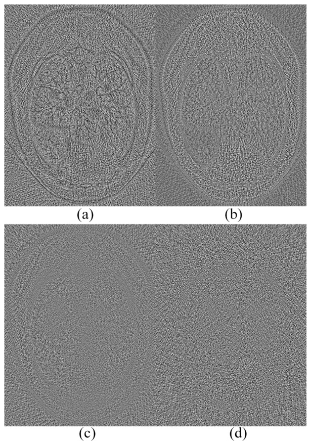
Difference images between the low-dose FBP image and the results using (a) ASD-POCS, (b) KSVD, (c) BM3D, and (d) CNN methods respectively.
4. Discussions and conclusion
Deep learning has achieved exciting results in the fields of computer vision and image processing, such as image segmentation, object detection, object tracking, image supper-resolution, etc. In medical imaging, deep learning has been so far applied in image analysis such as, segmentation and detection, and its potential for other applications has to be widely explored.
In this paper, a deep convolution neural network is presented to denoise images for low-dose CT. The proposed method learns a feature mapping from low- to normal-dose images. After the training stage, our method has achieved a competitive performance relative to the state-of-the-art methods in both qualitative and quantitative aspects. We have also assessed several factors for performance tradeoffs, suggesting the robustness of the proposed method at different noise levels and with respect to various training steps including the size of the training set. It is hypothesized that use of a deeper network with a larger capacity may further improve the performance, which we will investigate in the future.
Operating on 3D blocks should be an effective way to improve the performance of the proposed method. However, the goal of this initial paper is to demonstrate the effectiveness of deep learning. For this reason, operating on 2D patches is easier to implement and compare with other representative low-dose CT denoising methods, most of which were originally designed for 2D images. Clearly, training with 3D blocks will cost much more computational time, which will be pursued in our future work.
The computational cost of the proposed CNN based method needs to be commented on as well. The main cost of computational time is spent on the training stage. Although the training is normally done on GPU, it is still time-consuming. For a smaller training set with 200 images, about 106 patches were involved, and it took us 17 hours. For a larger training set with 2,000 images, about 107 patches were involved and 56 hours were spent. Other iterative methods do not need a training phase, but the execution time is much longer than the CNN based method. In this study, the average execution times (CPU mode) for ASD-POCS, KSVD, BM3D and CNN were 23.79, 40.88, 3.33 and 2.05 seconds respectively. Actually, once the network is trained offline, the CNN based method is much more efficient than the other methods in terms of real execution time.
In conclusion, we have been much encouraged by the excellent performance of the deep convolutional neural network approach in the case of noise reduction for low-dose CT. The results have demonstrated the potential of the CNN-based method for medical imaging. In the future, the proposed network structure will be refined, and adapted to handle other topics in CT imaging, such as few-view reconstruction, metal artifact reduction, and interior CT. Another possible direction is to investigate different hyper parameters of the network, especially the number of layers, and other network architectures to deal with these CT problems and other imaging tasks.
Funding
National Natural Science Foundation of China (NSFC) (61202160, 61302028, 61671312); National Institute of Biomedical Imaging and Bioengineering (NIBIB)/National Institutes of Health (NIH) (R01 EB016977, U01 EB017140).
References and links
- 1.Berrington de González A., Darby S., “Risk of cancer from diagnostic X-rays: Estimates for the UK and 14 other countries,” Lancet 363(9406), 345–351 (2004). 10.1016/S0140-6736(04)15433-0 [DOI] [PubMed] [Google Scholar]
- 2.Brenner D. J., Hall E. J., “Computed tomography- An increasing source of radiation exposure,” N. Engl. J. Med. 357(22), 2277–2284 (2007). 10.1056/NEJMra072149 [DOI] [PubMed] [Google Scholar]
- 3.Balda M., Hornegger J., Heismann B., “Ray contribution masks for structure adaptive sinogram filtering,” IEEE Trans. Med. Imaging 30(5), 1116–1128 (2011). [DOI] [PubMed] [Google Scholar]
- 4.Manduca A., Yu L., Trzasko J. D., Khaylova N., Kofler J. M., McCollough C. M., Fletcher J. G., “Projection space denoising with bilateral filtering and CT noise modeling for dose reduction in CT,” Med. Phys. 36(11), 4911–4919 (2009). 10.1118/1.3232004 [DOI] [PMC free article] [PubMed] [Google Scholar]
- 5.Li T., Li X., Wang J., Wen J., Lu H., Hsieh J., Liang Z., “Nonlinear sinogram smoothing for low-dose x-ray CT,” IEEE Trans. Nucl. Sci. 51(5), 2505–2513 (2004). 10.1109/TNS.2004.834824 [DOI] [Google Scholar]
- 6.Wang J., Lu H., Wen J., Liang Z., “Multiscale penalized weighted least-squares sinogram restoration for low-dose x-ray computed tomography,” IEEE Trans. Biomed. Eng. 55(3), 1022–1031 (2008). 10.1109/TBME.2007.909531 [DOI] [PubMed] [Google Scholar]
- 7.Tang S., Tang X., “Statistical CT noise reduction with multiscale decomposition and penalized weighted least squares in the projection domain,” Med. Phys. 39(9), 5498–5512 (2012). 10.1118/1.4745564 [DOI] [PMC free article] [PubMed] [Google Scholar]
- 8.Sidky E. Y., Pan X., “Image reconstruction in circular cone-beam computed tomography by constrained, total-variation minimization,” Phys. Med. Biol. 53(17), 4777–4807 (2008). 10.1088/0031-9155/53/17/021 [DOI] [PMC free article] [PubMed] [Google Scholar]
- 9.Zhang Y., Zhang W., Lei Y., Zhou J., “Few-view image reconstruction with fractional-order total variation,” J. Opt. Soc. Am. A 31(5), 981–995 (2014). 10.1364/JOSAA.31.000981 [DOI] [PubMed] [Google Scholar]
- 10.Zhang Y., Wang Y., Zhang W., Lin F., Pu Y., Zhou J., “Statistical iterative reconstruction using adaptive fractional order regularization,” Biomed. Opt. Express 7(3), 1015–1029 (2016). 10.1364/BOE.7.001015 [DOI] [PMC free article] [PubMed] [Google Scholar]
- 11.Zhang Y., Zhang W.-H., Chen H., Yang M.-L., Li T.-Y., Zhou J.-L., “Few-view image reconstruction combining total variation and a high-order norm,” Int. J. Imaging Syst. Technol. 23(3), 249–255 (2013). 10.1002/ima.22058 [DOI] [Google Scholar]
- 12.Chen Y., Gao D., Nie C., Luo L., Chen W., Yin X., Lin Y., “Bayesian statistical reconstruction for low-dose x-ray computed tomography using an adaptive-weighting nonlocal prior,” Comput. Med. Imaging Graph. 33(7), 495–500 (2009). 10.1016/j.compmedimag.2008.12.007 [DOI] [PubMed] [Google Scholar]
- 13.Ma J., Zhang H., Gao Y., Huang J., Liang Z., Feng Q., Chen W., “Iterative image reconstruction for cerebral perfusion CT using a pre-contrast scan induced edge-preserving prior,” Phys. Med. Biol. 57(22), 7519–7542 (2012). 10.1088/0031-9155/57/22/7519 [DOI] [PMC free article] [PubMed] [Google Scholar]
- 14.Zhang Y., Xi Y., Yang Q., Cong W., Zhou J., Wang G., “Spectral CT reconstruction with image sparsity and spectral mean,” IEEE Trans. Comput. Imaging 2(4), 510–523 (2016). 10.1109/TCI.2016.2609414 [DOI] [PMC free article] [PubMed] [Google Scholar]
- 15.Xu Q., Yu H., Mou X., Zhang L., Hsieh J., Wang G., “Low-dose x-ray CT reconstruction via dictionary learning,” IEEE Trans. Med. Imaging 31(9), 1682–1697 (2012). 10.1109/TMI.2012.2195669 [DOI] [PMC free article] [PubMed] [Google Scholar]
- 16.Cai J.-F., Jia X., Gao H., Jiang S. B., Shen Z., Zhao H., “Cine cone beam CT reconstruction using low-rank matrix factorization: algorithm and a proof-of-principle study,” IEEE Trans. Med. Imaging 33(8), 1581–1591 (2014). 10.1109/TMI.2014.2319055 [DOI] [PMC free article] [PubMed] [Google Scholar]
- 17.Chen Y., Yang Z., Hu Y., Yang G., Zhu Y., Li Y., Luo L., Chen W., Toumoulin C., “Thoracic low-dose CT image processing using an artifact suppressed large-scale nonlocal means,” Phys. Med. Biol. 57(9), 2667–2688 (2012). 10.1088/0031-9155/57/9/2667 [DOI] [PubMed] [Google Scholar]
- 18.Ma J., Huang J., Feng Q., Zhang H., Lu H., Liang Z., Chen W., “Low-dose computed tomography image restoration using previous normal-dose scan,” Med. Phys. 38(10), 5713–5731 (2011). 10.1118/1.3638125 [DOI] [PMC free article] [PubMed] [Google Scholar]
- 19.Li Z., Yu L., Trzasko J. D., Lake D. S., Blezek D. J., Fletcher J. G., McCollough C. H., Manduca A., “Adaptive nonlocal means filtering based on local noise level for CT denoising,” Med. Phys. 41(1), 011908 (2014). 10.1118/1.4851635 [DOI] [PubMed] [Google Scholar]
- 20.Aharon M., Elad M., Bruckstein A., “K-SVD: An algorithm for designing overcomplete dictionaries for sparse representation,” IEEE Trans. Signal Process. 54(11), 4311–4322 (2006). 10.1109/TSP.2006.881199 [DOI] [Google Scholar]
- 21.Chen Y., Yin X., Shi L., Shu H., Luo L., Coatrieux J.-L., Toumoulin C., “Improving abdomen tumor low-dose CT images using a fast dictionary learning based processing,” Phys. Med. Biol. 58(16), 5803–5820 (2013). 10.1088/0031-9155/58/16/5803 [DOI] [PubMed] [Google Scholar]
- 22.Fumene Feruglio P., Vinegoni C., Gros J., Sbarbati A., Weissleder R., “Block matching 3D random noise filtering for absorption optical projection tomography,” Phys. Med. Biol. 55(18), 5401–5415 (2010). 10.1088/0031-9155/55/18/009 [DOI] [PMC free article] [PubMed] [Google Scholar]
- 23.Sheng K., Gou S., Wu J., Qi S. X., “Denoised and texture enhanced MVCT to improve soft tissue conspicuity,” Med. Phys. 41(10), 101916 (2014). 10.1118/1.4894714 [DOI] [PubMed] [Google Scholar]
- 24.Kang D., Slomka P., Nakazato R., Woo J., Berman D. S., Kuo C.-C. J., Dey D., “Image denoising of low-radiation dose coronary CT angiography by an adaptive block-matching 3D algorithm,” Proc. SPIE 8669, 86692G (2013). 10.1117/12.2006907 [DOI] [Google Scholar]
- 25.Hinton G. E., Osindero S., Teh Y.-W., “A fast learning algorithm for deep belief nets,” Neural Comput. 18(7), 1527–1554 (2006). 10.1162/neco.2006.18.7.1527 [DOI] [PubMed] [Google Scholar]
- 26.Hinton G. E., Salakhutdinov R. R., “Reducing the dimensionality of data with neural networks,” Science 313(5786), 504–507 (2006). 10.1126/science.1127647 [DOI] [PubMed] [Google Scholar]
- 27.LeCun Y., Bengio Y., Hinton G., “Deep learning,” Nature 521(7553), 436–444 (2015). 10.1038/nature14539 [DOI] [PubMed] [Google Scholar]
- 28.Jain V., Seung H., “Natural image denoising with convolutional networks” in Proc. Adv. Neural Inf. Process. Syst. (NIPS, 2008), pp.769–776. [Google Scholar]
- 29.Dong C., Loy C. C., He K., Tang X., “Image super-resolution using deep convolutional networks,” IEEE Trans. Pattern Anal. Mach. Intell. 38(2), 295–307 (2016). 10.1109/TPAMI.2015.2439281 [DOI] [PubMed] [Google Scholar]
- 30.Xu L., Ren J. S. J., Liu C., Jia J., “Deep convolutional neural network for image deconvolution,” in Proc. Adv. Neural Inf. Process. Syst. (NIPS, 2014), pp. 1790–1798. [Google Scholar]
- 31.Xie J., Xun L., Chen E., “Image denoising and inpainting with deep neural networks,” in Proc. Adv. Neural Inf. Process. Syst. (NIPS, 2012), pp. 350–352. [Google Scholar]
- 32.Burger H. C., Schuler C. J., Harmeling S., “Image denoising: can plain neural networks compete with BM3D?” In Proceedings of the IEEE Conference on Computer Vision and Pattern Recognition (IEEE, 2012), pp. 2392–2399. 10.1109/CVPR.2012.6247952 [DOI] [Google Scholar]
- 33.Wang R., Tao D., “Non-local auto-encoder with collaborative stabilization for image restoration,” IEEE Trans. Image Process. 25(5), 2117–2129 (2016). 10.1109/TIP.2016.2541318 [DOI] [PubMed] [Google Scholar]
- 34.Agostinelli F., Anderson M. R., Lee H., “Adaptive multi-column deep neural networks with application to robust image denoising,” in Proc. Adv. Neural Inf. Process. Syst. (NIPS, 2013), pp. 1493–1501. [Google Scholar]
- 35.Liao S., Gao Y., Oto A., Shen D., “Representation learning: a unified deep learning framework for automatic prostate MR segmentation,” Med Image Comput Comput Assist Interv 16(2), 254–261 (2013). [DOI] [PMC free article] [PubMed] [Google Scholar]
- 36.Cha K. H., Hadjiiski L., Samala R. K., Chan H.-P., Caoili E. M., Cohan R. H., “Urinary bladder segmentation in CT urography using deep-learning convolutional neural network and level sets,” Med. Phys. 43(4), 1882–1896 (2016). 10.1118/1.4944498 [DOI] [PMC free article] [PubMed] [Google Scholar]
- 37.Kallenberg M., Petersen K., Nielsen M., Ng A. Y., Pengfei Diao C., Igel C. M., Vachon K., Holland R. R., Winkel N., Karssemeijer, Lillholm M., “Unsupervised deep learning applied to breast density segmentation and mammographic risk scoring,” IEEE Trans. Med. Imaging 35(5), 1322–1331 (2016). 10.1109/TMI.2016.2532122 [DOI] [PubMed] [Google Scholar]
- 38.Xu J., Xiang L., Liu Q., Gilmore H., Wu J., Tang J., Madabhushi A., “Stacked sparse autoencoder (SSDA) for nuclei detection of breast cancer histopathology images,” IEEE Trans. Med. Imaging 35(1), 119–130 (2016). 10.1109/TMI.2015.2458702 [DOI] [PMC free article] [PubMed] [Google Scholar]
- 39.Sirinukunwattana K., Ahmed Raza S. E., Yee-Wah Tsang D. R. J., Snead I. A., Cree, Rajpoot N. M., “Locality sensitive deep learning for detectionand classification of nuclei in routine colon cancer histology images,” IEEE Trans. Med. Imaging 35(5), 1196–1206 (2016). 10.1109/TMI.2016.2525803 [DOI] [PubMed] [Google Scholar]
- 40.Shin H. C., Orton M. R., Collins D. J., Doran S. J., Leach M. O., “Stacked autoencoders for unsupervised feature learning and multiple organ detection in a pilot study using 4D patient data,” IEEE Trans. Pattern Anal. Mach. Intell. 35(8), 1930–1943 (2013). 10.1109/TPAMI.2012.277 [DOI] [PubMed] [Google Scholar]
- 41.Wang S., Su Z., Ying L., Peng X., Zhu S., Liang F., Feng D., Liang D., “Accelerating magnetic resonance imaging via deep learning,” In Proceedings of the IEEE International Symposium on Biomedical Imaging (IEEE, 2016), pp. 514–517. 10.1109/ISBI.2016.7493320 [DOI] [PMC free article] [PubMed] [Google Scholar]
- 42.H. Zhang, L. Li, K. Qiao, L. Wang, B. Yan, L. Li, and G. Hu, “Image predication for limited-angle tomography via deep learning with convolutional neural network,” arXiv:1607.08707 (2016).
- 43.Wang G., “A perspective on deep imaging,” IEEE Access. in press., doi:. 10.1109/ACCESS.2016.2624938 [DOI]
- 44.E. Kang, J. Min, and J. C. Ye, “A deep convolutional neural network using directional wavelets for low-dose X-ray CT reconstruction,” arXiv:1610.09736 (2016). [DOI] [PubMed]
- 45.Candès E. J., Romberg J., Tao T., “Robust uncertainty principles: Exact signal reconstruction from highly incomplete frequency information,” IEEE Trans. Inf. Theory 52(2), 489–509 (2006). 10.1109/TIT.2005.862083 [DOI] [Google Scholar]
- 46.Elad M., Aharon M., “Image denoising via sparse and redundant representations over learned dictionaries,” IEEE Trans. Image Process. 15(12), 3736–3745 (2006). 10.1109/TIP.2006.881969 [DOI] [PubMed] [Google Scholar]
- 47.Nair V., Hinton G. E., “Rectified linear units improve restricted Boltzmann machines,” in Proc. Int. Conf. Mach. Learn. (IEEE, 2010), pp. 807–814. [Google Scholar]
- 48.Lecun Y., Bottou L., Bengio Y., Haffner P., “Gradient-based learning applied to document recognition,” Proc. IEEE 86(11), 2278–2324 (1998). 10.1109/5.726791 [DOI] [Google Scholar]
- 49.Wang Z., Bovik A. C., Sheikh H. R., Simoncelli E. P., “Image quality assessment: from error visibility to structural similarity,” IEEE Trans. Image Process. 13(4), 600–612 (2004). 10.1109/TIP.2003.819861 [DOI] [PubMed] [Google Scholar]
- 50.Siddon R. L., “Fast calculation of the exact radiological path for a three-dimensional CT array,” Med. Phys. 12(2), 252–255 (1985). 10.1118/1.595715 [DOI] [PubMed] [Google Scholar]
- 51.Jaitly N., Hinton G. E., “Learning a better representation of speech soundwaves using restricted Boltzmann machines,” In Proceedings of the IEEE Conference on Acoustics, Speech and Signal Processing . (IEEE, 2011), 5884–5887. 10.1109/ICASSP.2011.5947700 [DOI] [Google Scholar]
- 52.Li W., Duan L., Xu D., Tsang I. W., “Learning with augmented features for supervised and semi-supervised heterogeneous domain adaptation,” IEEE Trans. Pattern Anal. Mach. Intell. 36(6), 1134–1148 (2014). 10.1109/TPAMI.2013.167 [DOI] [PubMed] [Google Scholar]
- 53.Zhu J., Chen N., Perkins H., Zhang B., “Gibbs max-margin topic models with data augmentation,” J. Mach. Learn. Res. 15(1), 1073–1110 (2013). [Google Scholar]