Extinction pathways and outbreak vulnerability in a stochastic Ebola model

Abstract

A zoonotic disease is a disease that can be passed from animals to humans. Zoonotic viruses may adapt to a human host eventually becoming endemic in humans, but before doing so punctuated outbreaks of the zoonotic virus may be observed. The Ebola virus disease (EVD) is an example of such a disease. The animal population in which the disease agent is able to reproduce in sufficient number to be able to transmit to a susceptible human host is called a reservoir. There is little work devoted to understanding stochastic population dynamics in the presence of a reservoir, specifically the phenomena of disease extinction and reintroduction. Here, we build a stochastic EVD model and explicitly consider the impacts of an animal reservoir on the disease persistence. Our modelling approach enables the analysis of invasion and fade-out dynamics, including the efficacy of possible intervention strategies. We investigate outbreak vulnerability and the probability of local extinction and quantify the effective basic reproduction number. We also consider the effects of dynamic population size. Our results provide an improved understanding of outbreak and extinction dynamics in zoonotic diseases, such as EVD.

1. Introduction

The Ebola virus disease (EVD) is an infectious zoonosis found in several mammals, including humans, bats and apes. A zoonosis is a disease that can be naturally transmitted from animals to humans. If there is a non-human disease carrier, we call that species a disease reservoir. Strong evidence for an Ebola virus reservoir can be seen in the invasion/extinction cycles that have taken place over the 40 years of recorded EVD history in humans. The first known spillover of EVD into the human population took place in Zaire (now the Democratic Republic of the Congo) near the Ebola River from which the disease took its name. Major EVD epidemics have taken place in the Democratic Republic of the Congo, Gabon, Sudan, Uganda, and most recently in Guinea, Sierra Leone and Liberia. Although the disease was first recognized and has been primarily located in Central Africa, the most recent epidemic has been taking place along the continent's western coast.

Unlike non-zoonotic diseases, EVD goes through long periods of global extinction in the human population. These EVD-free periods are punctuated by seemingly spontaneous disease reintroduction, which suggests infection from a non-human source. Additionally, there is a large body of work in the biological and ecological sciences providing evidence that the virus is maintained in animal populations [1,2]. Thus, the seemingly spontaneous reappearance of the disease in the human population must be understood in the context of unpredictable interactions between humans and animal carriers of the disease. Although they are random in nature, researchers are working to improve our understanding of these interactions [3,4].

The EVD is transmitted via bodily fluids such as blood, saliva, semen and breast milk, and is very deadly in both humans and apes, with an average mortality rate of 50% in humans. Depending on the viral strain, the disease may kill as much as 90% of an affected human population [5]. When the disease is transferred from the animal reservoir into the human population it is known as a spillover event. Although EVD has a relatively difficult time invading and persisting in a human population, there have been over half a dozen spillover events with more than 100 infected individuals since 1976, when the disease was initially recognized in Zaire (now the Democratic Republic of Congo). The Centers for Disease Control and Prevention (CDC) in the USA estimates over 28 000 infections and over 11 000 deaths in the most recent West African epidemic [6]. As of March 2016, the epidemic is under control with small on-going flare-ups that are likely to continue to occur for the immediate future.

From a modelling perspective, considering an estimated disease incubation time of 7–21 days, a deterministic susceptible–exposed–infectious–recovered (SEIR) compartmental model is appropriate to investigate the dynamics [7–9]. Extensions have been proposed to account for various kinds of intervention [10] or, as in the case of gravity models, to account for the spread of EVD over an explicit spatial region. In a gravity model, the force of infection from a non-contiguous population will be proportional to the size of the respective populations, and inversely proportional to the square of the distance between the two populations [11,12].

Studies that explicitly consider the dynamics of EVD while in the presence of a zoonotic reservoir are less common. Although the zoonotic reservoir for Ebola is still a matter of contention among researchers, bats make for a likely suspect [1,2]. It is known that non-human primates are sometimes involved in the spread of EVD to humans as intermediate susceptible hosts [3]. Accounting for human exposure to the reservoir is paramount for the study of disease introduction. However, disease extinction and reintroduction are rare stochastic events that cannot be captured by deterministic models.

Therefore, the goal of this paper is to present a stochastic model that explicitly accounts for both the introduction of EVD from the zoonotic reservoir as well as the fade-out periods. Perturbations of this work can be used to assess the efficacy of disease control strategies such as vaccination and quarantine. Additionally, the work supports the use of the basic reproduction number while quantifying outbreak vulnerability in populations weakly coupled to a disease reservoir. Although this paper focuses on EVD, the results are broadly relevant to outbreak and extinction in zoonotic diseases.

2. Material and methods

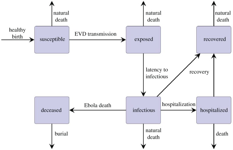
In this paper, we extend a previously adopted compartmental model for EVD with intervention [10] to a stochastic model that captures the internal random dynamics of a population. Figure 1 shows the division of the population into the following six classes:

• (1) Susceptible class S consists of individuals who may become infected with EVD through contact with an infectious individual, a hospitalized individual, or a deceased but unburied individual.

• (2) Exposed class E consists of individuals who are infected with EVD but are not yet infectious.

• (3) Infectious class I consists of individuals who are capable of transmitting EVD to a susceptible individual.

• (4) Recovered class R consists of individuals who have recovered from EVD.

• (5) Deceased class D consists of deceased and unburied individuals who are capable of transmitting EVD to a susceptible individual.

• (6) Hospitalized class H consists of individuals who have been hospitalized and are capable of transmitting EVD to a susceptible individual. In our model, we assume that individuals who die while in the hospitalized class are immediately buried.

Figure 1 also shows the interactions among these population classes. Note that EVD transmission can occur through both infectious human contact and the animal reservoir. We assume that contact with the animal reservoir is always possible, and independent of the ratio of animal carriers to humans.

Figure 1.

Flow diagram for the EVD model. (Online version in colour.)

The model we study is an extension of an SEIR model. Besides explicit consideration of the reservoir, the model includes two additional classes: hospitalized and deceased. We note that this model (without a reservoir) has been used in previous studies [9,10]. The hospitalized and deceased compartments account for important routes of disease transmission which are specific to EVD. Additionally, these routes provide a way to investigate the usefulness of practical intervention through the rate of hospitalization and fast access to a safe burial. The effectiveness of practical intervention strategies can be monitored through these parameters, together with variations in contact rates.

The model captures movement between the classes as stochastic transitions that occur at specified transition rates. Each of these transitions represents a random event that can occur in a population. Table 1 quantifies the possible transition events and associated rates, which follow the figure 1 flow diagram. In the master equation approach to stochastic modelling, these transition rates are used as coefficients that define the probability of each respective transition event [13,14]. Assuming some discrete period of time during which exactly one of the aforementioned events takes place, the probability that a particular event will be the one that does take place is equal to its own transition rate divided by the sum of all transition rates. The stochastic simulations reported on in this paper use these transitions in a Monte Carlo algorithm as described in [15].

Table 1.

The transition events and their associated transition rates for the stochastic EVD model. Each transition involves the movement of a single individual between classes. The classes are represented by the following variables: S = susceptible, E = exposed, I = infectious, R = recovered, H = hospitalized and D = deceased. The average population size is N.

event	transition	rate
healthy birth	Ø → S	μ N
EVD transmission (human)	S → E	(
EVD transmission (animal)	S → E	κ S
latency to infectious	E → I	σ E
recovery	I → R	γir I
EVD death	I → D	μe I
hospitalization	I → H	τ I
burial	D → Ø	δ D
death from hospital	H → Ø	μe H
recovery from hospital	H → R	γhr H
natural death	{S,E,I,D,H,R} → Ø	μ{S,E,I,D,H,R}

The parameter values we use for EVD are given in table 2. With the exception of κ, the parameters are as reported in [10]. The value of κ defines the probability of an infection from the animal reservoir. The approximate range for κ can be calculated by dividing the number of outbreak events by the time over which those outbreaks took place and then dividing by the population size. This gives an approximate range for κ between 10⁻⁹ and 10⁻⁶.

Table 2.

The parameter values used in the stochastic EVD model, as reported in [10].

description	parameter	value
1/host life span (and birth rate)	μ	0.00005 d−1
contact rate for infectious	βi	0.5 d−1
contact rate for deceased	βd	0.6 d−1
contact rate for hospitalized	βh	0.00016 d−1
1/latency period	σ	0.1 d−1
1/recovery period (no hospital)	γir	0.07 d−1
death rate from EVD	μe	0.12 d−1
1/mean time to hospitalization	τ	0.2 d−1
1/burial time	δ	0.33 d−1
1/recovery period (hospital)	γhr	0.10 d−1
reservoir transmission	κ	5 × 10−9 d−1

In both the earlier and the more recent EVD outbreaks in Africa, the virus has been reported to have relatively low infectivity [8,16]. A common metric for infectivity of a disease is the basic reproduction number, R₀, which is defined as the average number of infections that a single infectious individual will trigger in a fully susceptible population. R₀ can be described more roughly as the ratio between the inflow of infected individuals and the outflow of dead or recovered individuals in a fully susceptible population. If the inflow is greater than the outflow, then R₀ > 1, and the disease will spread. If the outflow is greater than the inflow, then R₀ < 1, and the disease will go extinct. For context, the reproductive number for measles may be as high as R₀ = 18 and the reproductive number for influenza is R₀ ≈ 4. The reproductive number for EVD is estimated to be approximately R₀ ≤ 2 [8,16]. The parameters in table 2 agree with this estimation.

If the transitions between states are short and uncorrelated and we assume the population is well mixed, the system is a Markov process and the evolution of the probability is described by a master equation [13,14]. We assume that the population is large and the WKB (Wentzel–Kramers–Brillouin) approximation for the probability distribution in the scaled master equation can be used [17–21]. By performing a Taylor series expansion on this equation, one arrives at the leading-order Hamilton–Jacobi equation for which the stochastic dynamics are captured in the conjugate momentum variables. This statistical mechanics approach to the problem naturally leads to the associated Hamiltonian and Hamilton's equations, which doubles the dimension of the problem but recasts it as a deterministic system of nonlinear differential equations that is useful to analyse the dynamics of the original stochastic system [22–24]. The master equation and Hamiltonian for the stochastic EVD model are provided in appendix A.

The standard approach to analysing the dynamics of a stochastic system such as this is to start with the mean-field equations (provided in appendix B). This is done by assuming a value of zero for the conjugate momentum variables in Hamilton's equations. This reduced system captures the deterministic dynamics, which is the limit of the stochastic dynamics in the large population limit. Full analysis of the mean-field equations for the EVD model reveals dynamics similar to lower dimensional SEIR systems in the literature [7]. Two steady states of the mean-field equations can be derived analytically. If we assume no reservoir transmission (κ = 0), the first steady state can be described as the disease-free equilibrium (DFE), for which the entire population is susceptible and no infection is present. This state is stable if the basic reproduction number satisfies R₀ < 1, implying that the disease cannot persist in the population and all solutions will limit to the DFE. If R₀ > 1, the DFE is unstable and the disease will persist. In other words, if EVD is introduced into a system having R₀ > 1, solutions will tend to an endemic steady state, implying non-zero values for the infected and infectious classes.

By introducing reservoir transmission (κ > 0), the traditional DFE no longer exists as a small number of exposed individuals are introduced to the system. Therefore, in addition to the traditional endemic state, there is another steady state that we call the invasion state that has a small number of non-susceptible individuals. While this deterministic system cannot exhibit periods of disease fade-out and re-invasion, its steady states provide guidance in understanding the dynamics of the full stochastic system. The existence of the invasion state depends on the force of infection from the animal reservoir, and we will see that it plays an important role in outbreak vulnerability.

Another advantage of analysing the mean-field equations is the ability to approximate the basic reproduction number. Using the next-generation matrix as described in [25] and assuming no reservoir transmission (κ = 0), we use the DFE to analytically determine

2.1

which quantifies whether EVD can persist in the population. The derivation for the basic reproduction number is provided in appendix C. Because the reservoir transmission is small, this quantity provides a good approximation of the ability for the disease to persist when randomly introduced. Intervention methods can also be evaluated by how they decrease this value, with an aim of R₀ < 1.

3. Results

Real-world data for EVD suggest that the basic reproduction rate is greater than one, but the disease dynamics cannot be captured by deterministic models with solutions that simply limit to a steady state. The stochastic EVD model allows behaviour beyond the dynamics predicted by the mean-field equations. Examples include solutions that switch steady states, resembling disease outbreak (invasion) and fade-out (extinction) events. In particular, we are interested in the effect of a transmission reservoir in these dynamics.

3.1. Invasion

We begin by discussing outbreak vulnerability in the stochastic EVD model, which describes the invasion dynamics after an infected individual is introduced into a population having few or no infections. The random introduction would occur through the transmission reservoir, quantified by the parameter κ. While the larger infrequent outbreaks would result in an under-prepared and overwhelmed healthcare system, the impact of long, sustained outbreaks would be more taxing on a population. Assessing the outbreak vulnerability of a specific population and the effectiveness of possible intervention strategies would help prepare healthcare workers and possibly prevent a breakdown of the system during an outbreak.

Representative time series for several reservoir transmission rates using EVD parameters are presented in the inlay of figure 2. If there is very low transmission from the reservoir and most of the population is susceptible, the solution will exhibit large outbreaks, or spillover events, spread out in time so that there are long disease-free periods. This behaviour is represented by the green time series in the inlay of figure 2. If the transmission rate from the reservoir is high, then the solution oscillates about a non-zero steady state and there are few if any disease-free periods. This behaviour is represented by the red time series in the inlay of figure 2. The colour bar at the bottom of figure 2 shows the values for κ exhibiting these dynamics and how a combination of these two green and red extremes is exhibited by solutions for transmission rates in between. The orange time series in the inlay is presented as a representative example.

Figure 2.

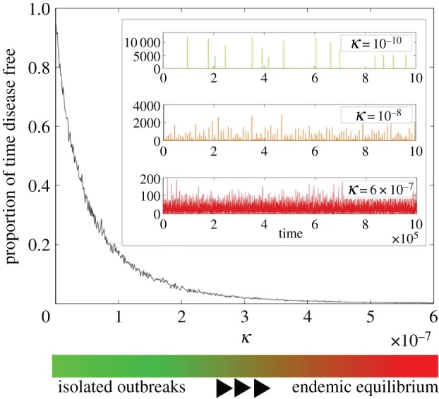
A measure of outbreak vulnerability as a function of the reservoir transmission rate κ. The figure, based on 10³ stochastic simulations run for 10⁶ days for a population N = 500 000, shows the proportion of disease-free time for a given κ. The inlay shows three representative time series of the number of cases of EVD over a sample of 10⁵ days. All parameters are set to the values in table 2 except κ, which is noted in each graph.

We measure the outbreak vulnerability of the system by finding the average proportion of disease-free time during a sample of 1000 stochastic simulations. Details regarding the numerical simulations can be found in appendix D. The results for EVD parameters as we vary κ are presented in figure 2. For populations with very weak connection to the disease reservoir (small κ), almost all of the time is spent disease free. As κ increases, the disease-free time decreases at a nearly exponential rate. We describe the periods of disease-free time as disease fade-out and the decrease of fade-out is associated with sustained outbreaks.

Both the contact rate with infected individuals (β_i) and the EVD burial rate (δ) are important factors for a population's outbreak vulnerability and can change over the course of an outbreak, as they relate to human behavioural considerations that are likely to be affected by the spread of information. One would assume that increasing δ and decreasing β_i would be salient and practical strategies to reduce outbreak vulnerability. The stochastic EVD model can provide an estimate of how the outbreak vulnerability changes with these prevention measures, allowing for the assessment of how to achieve the maximum impact. Figure 3 is a graph of the average proportion of disease-free time in simulations of the EVD model as β_i and δ are varied. These simulations follow the methodology described for figure 2. As expected, low values for the contact rate and high values for the burial rate have the most disease-free time and least outbreak vulnerability. Overlaid as a dashed black curve is R₀ = 1 for the mean-field EVD model without reservoir transmission, as described in equation (2.1). This curve is the boundary between the basins for which the DFE and the endemic steady states are stable in the mean-field EVD model. When R₀ < 1, the DFE is stable for low values for the contact rate and high values for the burial rate. We propose to use the R₀ = 1 curve to approximate the boundary between low and high outbreak vulnerability in the stochastic EVD model with reservoir transmission. Therefore, it indicates intervention strategies that target β_i and δ parameter values for R₀ < 1 (below the dashed line) which would have the greatest benefit for the population.

Figure 3.

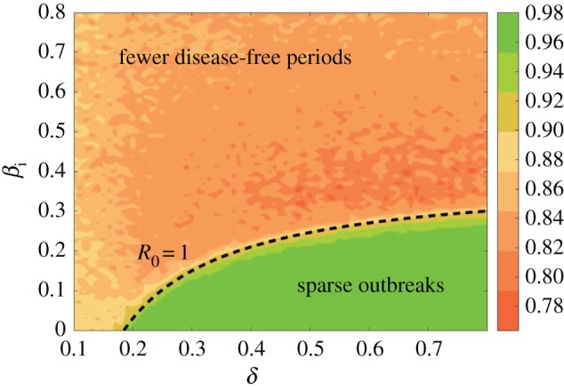
A measure of intervention effectiveness considering the impact of limiting the contact rate with infectious individuals β_i and increasing the burial rate for deceased EVD individuals δ. The figure shows a contour plot of the proportion of disease-free time for simulations as described in figure 2 with parameters given in table 2 and a population N = 500 000. Higher values (green) represent infrequent outbreaks with long periods that are disease free. Lower values (red) represent few disease-free periods and sustained outbreaks. Overlaid as a dashed black curve is R₀ = 1 for the mean-field EVD model without reservoir transmission, as described in equation (2.1).

3.2. Extinction

We continue with a discussion of how the stochastic EVD model can exhibit periods of disease absence, or fade-out, despite the fact that the basic reproduction rate is greater than one. As we have noted in the previous section, outbreaks can be quick and infrequent or sustained and frequent, depending on outbreak vulnerability. This distinction describes the two mechanisms that allow for a solution to reach a disease-free state, which we consider an extinction event.

When the outbreak vulnerability is low, there are long disease-free periods in which the susceptible population replenishes itself as the recovered individuals are naturally removed. The small transmission rate from the reservoir has a low probability of causing an outbreak, and finally, when it happens, the susceptible compartment is the majority of the population and the disease quickly spreads through the group. Here, the mean-field model provides general insight for the underlying dynamics exhibited by the stochastic model. The stable endemic state (assuming R₀ > 1) is a spiral sink and solutions spiral in towards it in an anticlockwise fashion when projected on the susceptible–infectious plane. The initial conditions for the invasion are far from the endemic state, which is stable but not strongly attracting (1 < R₀ < 2). Therefore, the solution will orbit the endemic state in a large anticlockwise path (at a significant distance from the endemic state), quickly reaching a disease-free state on the other side of the orbit. The solution will remain disease free as the susceptible population rebuilds and repeats the cycle. These outbreaks are random, but, as shown in figure 3, the average behaviour follows a continuous measure of disease-free time that depends on the system parameters. It is worth mentioning that the invasion steady state is small and does not seem to play a significant role in these dynamics.

For large outbreak vulnerability, the invasion is a solution that escapes the disease-free state and causes a large disease outbreak. In this case, the solution is similar to what one would expect from the deterministic mean-field equations. What is unique about stochastic systems is that the small random fluctuations allow escape from steady states, and in simulations this will happen in finite time (although the time may be exponentially long). To understand the mechanism of escape, one can use Hamilton's equations to identify the quasi-stable steady states in the stochastic system, as well as action-minimizing curves that provide a path from one steady state to another. An action-minimizing curve identifies the path that is probabilistically most likely to be taken during a switching event. This trajectory is thus known as the optimal path [19,23,26,27]. For the EVD model, the optimal path to extinction is a curve in 12-dimensional space that connects the endemic state to the invasion state.

Noting that κ is much smaller than the other parameters in table 2, solutions for the stochastic EVD model near the endemic state can be approximated by assuming κ = 0. The exception is during invasion events, when the reservoir brings the disease back from extinction. Therefore, we set κ = 0 in an illustrative example for computing the optimal path to extinction and comparing it with extinction dynamics in simulations.

For this high-dimensional model, an analytic solution is not tractable and we use numerical methods to approximate the optimal path. We use the iterative action minimizing method (IAMM) [28] to find 2400 points approximating the 12-dimensional optimal path of the stochastic EVD model, with a maximum error of 2.4487 × 10⁻¹⁰. Details regarding the numerical simulations can be found in appendix E. Figure 4 shows the resulting solution, starting at the endemic state and spiralling out to the disease-free state. We verify our result by comparing it with the probability density of extinction prehistory in the susceptible–infectious plane. The probability density was numerically computed using 10 000 simulations that ended in spontaneous extinction (details in appendix D). Starting at the extinction point, the previous positions in state space for each trajectory are binned and the frequency is plotted in the susceptible–infectious plane in figure 4. The highest frequency regions are shown in red in the density plot, and the optimal path is overlaid. Figure 4 shows that, among all the paths the stochastic system can take to reach the extinct state, there is one path that has the highest probability of occurring. This optimal path of extinction lies on the peak of the probability density of the extinction prehistory.

Figure 4.

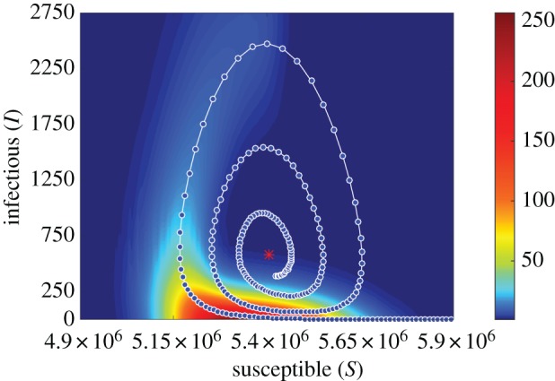
An optimal extinction path for a stochastic EVD system with κ = 0 and parameters given in table 2. The blue points represent the numerical approximation of the optimal path to extinction found by the IAMM. The path is overlaid on the probability density of extinction prehistories for 10 000 stochastic realizations for a population N = 10 000 000. Red indicates the highest frequencies.

Additional verification of the optimal path to extinction is achieved by projecting the 12-dimensional optimal path onto the lower-dimensional stochastic centre manifold shown in figure 5. Since the stochastic EVD model is an SEIR-type model, it is straightforward to compute the stochastic centre manifold from the mean-field equations using techniques developed in [29,30]. The stochastic centre manifold is the surface on which the long-term dynamics of the stochastic system will fall. Therefore, it follows that the approximation of the optimal path should lie on this hyperplane. The entire set of optimal path data and the centre manifold equation for the stochastic EVD model are provided in appendix E.

Figure 5.

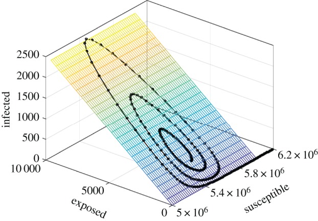
The projection of the numerically computed optimal path to extinction on the analytically determined stochastic centre manifold. Details for the computation are provided in the text. Parameter values are given in table 2, with κ = 0.

Knowledge of the optimal path is also useful, because it allows one to find the average time to travel from the endemic state to the extinct state. We call this time the mean time to disease extinction (MTE). Since the optimal path can be used to estimate the MTE it is useful for quantifying the efficacy of disease control such as vaccine and quarantine. In particular, an effective disease control programme will shift the optimal path in a way that decreases the MTE. Although this was not computed for the stochastic EVD model, it is straightforward both to track the extinction time during a simulation as well as to compute an expected mean value based on the optimal path. This will be a topic of future study.

For outbreak vulnerability parameters in between the two extremes, the system may exhibit a combination of quick and sustained outbreaks, sometimes using the optimal path to escape from the endemic state. The MTE may provide insight to the frequency of disease-free periods and may also provide a measure of intervention effectiveness.

3.3. Dynamic population size

Currently, we account for births and deaths in such a way that it is assumed that the stochastic EVD model retains a mean population size. While population growth rates in many African regions have declined steadily over time, the overall growth in Africa remains a net positive, with the population of many countries expected to double by the year 2050 [31,32]. When the birth rate is greater than the death rate, the total population will change in time. If we allow for a dynamic population size in the model, then both the endemic state and the basic reproduction rate become dynamic. Higher birth rates increase the flow of susceptible individuals into the population, which increases the probability of stochastic reintroduction and the force of infection. Consequently, the likelihood of stochastic fade-out decreases and the system is bound to transition to a dynamic endemic state. This implies that, even for the subcritical initial dynamic condition R₀ < 1, a transition to endemic disease circulation is likely. Moreover, it is dependent on various measures including both κ and birth rate. This condition, when realized, may limit the impact of intervention. We reserve the discussion of the linkage among these effects to another publication. By maintaining the natural death rate for all compartments at the value given in table 2, and increasing the birth rate to μ = 9.5 × 10⁻⁵, one can compute stochastic realizations of this dynamic process. Details regarding the numerical simulations can be found in appendix D. An example is shown in figure 6, where one can see that there is a fundamental change in behaviour. Initially, the population is relatively small and invasion events are infrequent, as shown by the red curve. Later in time, the inflow of susceptibles causes a shift to a persistent but increasing endemic state. Outbreak vulnerability has increased with population size, transitioning from infrequent to sustained outbreaks.

Figure 6.

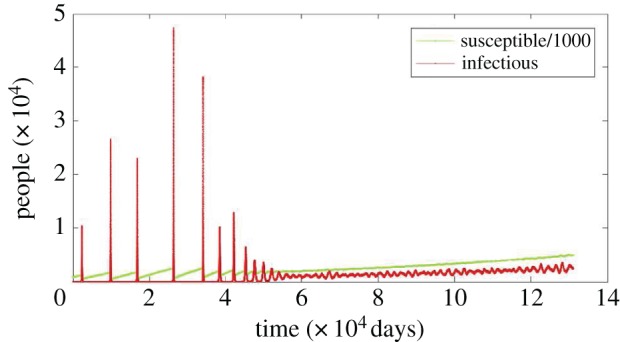
A growing population increases outbreak vulnerability and allows for sustained outbreaks. We show a sample time series with increasing population size (birth rate μ = 9.5 × 10⁻⁵ and κ = 1.8 × 10⁻⁹), and a starting population of N = 10⁶. The susceptible population has been scaled by a factor of 1000 so that both the infectious and susceptible time series can be clearly seen in the figure. Initially, the reservoir transmission triggers large outbreaks and results in fast extinction events. As the size of the population and the number of susceptible individuals increases, infectious individuals tend to a dynamic endemic state with sustained outbreaks. All other parameters are as in table 2.

4. Conclusion

The recent West African epidemic of EVD was a catastrophe that resulted in a devastating loss of life. With its frighteningly low survival rate, along with our apparent inability to predict the disease introduction and trajectory, EVD poses a continuing threat. For any such zoonosis disease, prevention prior to introduction is as important as disease control during an outbreak, and so the disease must be taken as seriously during its latent period as it is during an active period. In this paper, we contend that EVD should be considered in a stochastic framework and not as an entirely predictable deterministic process. The study of zoonotic diseases benefits particularly from the application of stochastic modelling methods because of the unpredictable nature of the human-to-reservoir interactions.

The optimal path to disease extinction is a minimal action trajectory between an endemic and extinct state. This path is the most likely route to disease extinction in the presence of noise. The optimal path can therefore be used to estimate the mean time to disease extinction, and as a result may be used to quantitatively assess disease control measures.

When a disease intervention strategy is adopted, it will affect the optimal path and the expected time to disease extinction. To determine an optimal intervention strategy, one must quantitatively compare different possible control methods. Control through an investigation of the optimal path has been successfully adopted in biochemical network dynamics [33]. The mean time to extinction, as determined through the optimal path, is the quantitative metric that should be used to determine the efficacy of a control method. In particular, studying the relationship between the optimal path and disease intervention may allow for the optimal allocation of resources prior to or during an epidemic. For example, Khasin et al. [34] identified the resonant effect of vaccination pulses in an SIR model and derived an optimal vaccination protocol that can speed up extinction when the vaccine is in short supply. Billings et al. [35] considered the effect of treatment for the SIS model, and showed an exponential decrease in disease extinction times.

In the case of the EVD model considered in this paper, the optimal path is a curve through 12-dimensional space, and is found by solving a 12-dimensional system of differential equations. Knowledge of the optimal path to extinction allows one to perturb our model to determine relative sensitivity to changes in human behaviour and to disease control strategies. With these tools, one could predict the relative effectiveness of disease control measures. Given appropriate cost functions for the implementation of the different control measures, one could minimize the mean time to extinction given a finite set of resources, thus developing an optimal strategy.

Once disease extinction has been achieved, then the Ebola virus will only be found in non-human populations and an understanding of the conditions for which invasion and outbreak are most likely can help us to identify at-risk populations. It can be seen using stochastic simulation techniques that there are populations where long-lived endemic states are very unlikely. This means that the disease may invade consistently, but is always driven down to extinction in a relatively short amount of time. Human behaviour as well as the attributes of the disease can affect the vulnerability of a population to outbreak. One way to quantify this risk is by using the basic reproduction number from the associated deterministic system. We have also observed that in a dynamic population size model, where the birth rate is larger than the death rate, the ability of the disease to invade into a population is dependent on the size of the population.

Figure 3 shows that the basic reproduction number from the deterministic system can be used as an indicator for stochastic outbreak vulnerability. This fact allows one to extend important conclusions from the investigation of deterministic systems to more realistic stochastic systems. We show the intuitive conclusion that increasing the burial rate and decreasing the contact rate will, ultimately, result in controlling the disease. The frequencies that are reported in figure 3 show how the presence of the reservoir impacts the probability of controlling the outbreak through standard intervention methods (self- or forced isolation and safe removal of infected bodies), while also affording information about which parameter may be more appropriate to modify in order to decrease the impact of the disease. It is worth noting that, in figure 3, the darker orange coloration in the region of medium contact rates and high burial rates is not a consequence of the model, but is rather due to the population size and number of stochastic realizations. An increase in either decreases the variance and results in a smoother, more even coloration.

Since the size of the endemic state scales proportionally with the size of the total population, larger populations tend to be more susceptible to a long-lived endemic state than smaller populations. Consider the number of infectious individuals at the endemic state as given in appendix B. As N increases, I increases proportionately. The deterministic system can never escape from the stable endemic state, regardless of how large or small the endemic state is. In the stochastic formulation, however, the endemic state becomes quasi-stable. This means that the natural variance of the stochastic system can force a transition between the endemic and extinct states. This favourable transition is less and less likely to happen as the population size increases. In fact, the mean time to stochastic extinction as a function of population size is known to be exponential. Therefore, larger populations are more likely to have a persistent disease after an invasion event than are smaller populations. Figure 6 shows that, as the population size increases over time, the risk for an endemic disease state increases as well. This suggests that the risk for disease invasion is particularly dynamic in developing areas. Population growth is expected to continue for decades in the developing world. The population of many African countries is predicted to double by 2050 [31,32]. Figure 6 shows that even a population with an endemic state small enough so that it will not be realized, but with a growing population, may overcome a threshold and suddenly display an endemic disease state after a long period of population growth. Although it is not explicitly investigated here, we hypothesize that a similar effect may be seen in an increasingly interconnected and globalized region. In theory, the phenomenon requires population growth, not necessarily from an imbalance between the birth and death rates. In the future, similar work should be done on a grid of interconnected populations, and in this way both spatial spread, which is not considered here, and increased interconnectedness among populations can be investigated.

Appendix A. Master equation and Hamiltonian

The six classes for the stochastic EVD model are represented by the following variables: S = susceptible, E = exposed, I = infectious, R = recovered, H = hospitalized and D = deceased. The general form of the master equation as described by the transitions in table 1 is

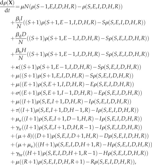A 1

where X =[S,E,I,D,H,R]^T.

We scale the variables by the average population size as follows: x_S = S/N, x_E = E/N, x_I = I/N, x_D = D/N, x_H = H/N, and x_R = R/N. The Hamiltonian for the stochastic EVD model using the WKB approximation is

A 2

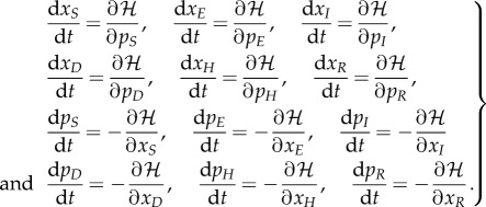
The associated Hamilton's equations are found by the relations:

A 3

The full equations for the EVD model are

A 4a

A 4b

A 4c

A 4d

A 4e

A 4f

A 4g

A 4h

A 4i

A 4j

A 4k

and

A 4l

Appendix B. Mean-field equations

To find the mean-field equations for the stochastic EVD model, one must evaluate the following partial derivatives of the Hamiltonian with the conjugate momentum variables set to zero (noted by p = 0):

B 1

The deterministic mean-field dynamics are given by the following equations:

B 2a

B 2b

B 2c

B 2d

B 2e

and

B 2f

Setting the deterministic mean-field equations to zero allows one to find the two steady states of the system in terms of the exposed variable. The exposed class value for the endemic state is

B 3

and the exposed class value for the invasion state is

B 4

Note that R₀ is the basic reproduction number whose definition and derivation is provided in appendix C. The values for the remaining variables of the steady states can be determined using the following relationships:

B 5

B 6

B 7

B 8

and

B 9

It is worth noting that if there is no transmission from the reservoir, or κ = 0, the form of the steady states for the exposed class simplifies to

B 10

We refer to the solution associated with x_E⁽ⁱ⁾ as the DFE:

B 11

Appendix C. Next-generation matrix and R₀

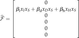
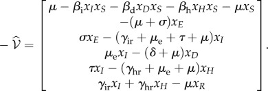
For deterministic systems, the basic reproduction number R₀ can be found explicitly using the next-generation matrix [25]. When κ > 0, the DFE does not exist so we proceed by assuming κ = 0. We rewrite the mean-field equations (equation (B 2)) using the vector , so that the new infections are separated from the other changes in the population using the form , with

C 1

and

C 2

We can reduce the system to the classes that have disease transmission using and defining , with

C 3

and

C 4

The vector represents all new infectives, and the vector is the negative of the remaining terms in the system.

We evaluate the Jacobian matrices of and at the DFE, called and , respectively. We then evaluate FV⁻¹, known as the next-generation matrix. Note that this expression captures the ratio between the inflow and an outflow from the infected classes in terms of matrix operations. The basic reproduction number is defined as the spectral radius (largest eigenvalue) of FV⁻¹:

C 5

Appendix D. Numerical simulations

Large collections of stochastic realizations, known as stochastic ensembles, were used to create figures 2–4. Each individual stochastic realization represents a possible disease trajectory and is produced using a type of Monte Carlo method [15]. The algorithm uses a random number generator to determine which event will occur as well as the time of occurrence. During each random time step exactly one event occurs. The probability of any particular event taking place is equal to its own transition rate divided by the sum of all transition rates. In the case of figure 6, the Spatiotemporal Epidemiological Modeler (STEM) was used. Different from all of the other simulations where the natural birth rate (μ) was equal to the natural death rate (μ), the creation of figure 6 involved setting the birth rate higher than the death rate so that μ_birth > μ_death. This is the mechanism that allows for an increasing population. Details of the numerical code can be found at http://wiki.eclipse.org/Ebola_Models.

The deterministic mean-field formulation of the EVD system given by equations (B 2) is solved using the Matlab Runge–Kutta solver ode45. Note that equations (B 2) are written in terms of the scaled variables . The scaled variables are the original variables (S,E,I,D,H,R) scaled by the average population size N. For the parameters given in table 2, the steady-state solutions are quite small. In particular, the endemic state of corresponds to for a population of N = 100 000 individuals. The reproductive number R₀ ≈ 1.84 agrees well with the value expected based on the literature, as was discussed in §2. Details of the numerical code can be found at https://www.eclipse.org/forums/index.php/t/1083337/.

Appendix E. Optimal extinction path

To analyse the dynamics of spontaneous escape from an endemic state, we numerically compute the optimal path, which is a zero-energy curve for the Hamiltonian that connects two steady-state saddle points. We use the IAMM [28], a numerical scheme based on Newton's method. The IAMM is useful in the general situation where a path connecting steady states C_a and C_b starts at C_a at and ends at C_b at . A time parameter t exists such that . For this method, we require a numerical approximation of the time needed to leave the region of C_a and arrive in the region of C_b. Therefore, we define a time such that . Additionally, and . In other words, the solution stays very near the equilibrium C_a for , has a transition region from , and then stays near C_b for . The interval is discretized into n segments using a uniform step size or a suitable non-uniform step size h_k. The corresponding time series is .

The derivative of the function value is approximated using central finite differences by the operator given as

E 1

Clearly, if a uniform step size is chosen, then equation (E 1) simplifies to the familiar form given as

E 2

Thus, one can develop the system of nonlinear algebraic equations

E 3

which is solved using a general Newton's method. We let

E 4

be an extended vector of 2nN components that contains the jth Newton iterate, where N is the number of populations. When j = 0, provides the initial ‘guess’ as to the location of the path that connects C_a and C_b. Given the jth Newton iterate q_j, the new q_j+1 iterate is found by solving the linear system

E 5

where F is the function defined by equation (E 3) acting on q_j, and J is the Jacobian. Equation (E 5) is solved using lower upper (LU) decomposition with partial pivoting.

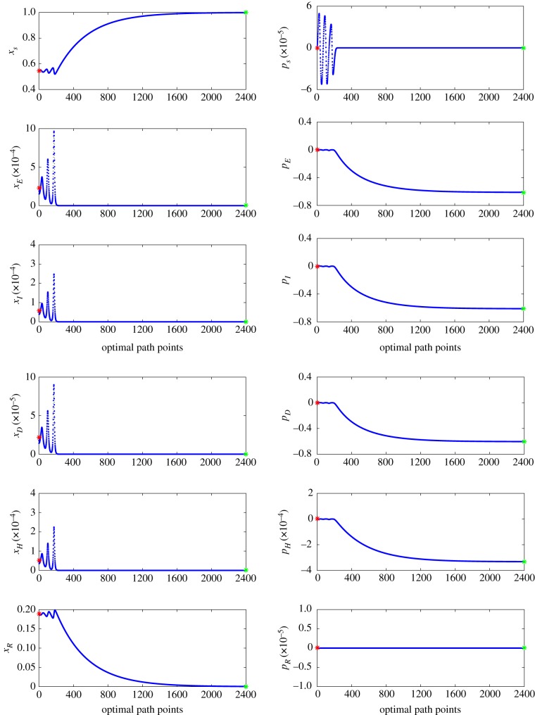
Because the endemic state of the mean field for the parameters in table 2 is a spiral sink, one must use a continuation method to find the optimal path. This is done by picking a large value of μ that results in an R₀ close to but larger than one, which decreases the frequency of the oscillations about the endemic state. Therefore, the optimal path can be found using an initial condition of a straight line connecting the endpoints. By slowly decreasing the value of μ and using the previous optimal path as the initial condition, one can repeat the process to find the optimal path at the desired parameter values. In figure 7, we present the entire set of data for the optimal extinction path for a stochastic EVD system shown in figure 4.

Figure 7.

The parameters are given in table 2, with the exception of κ = 0. Each set of 2400 blue points represent the numerical approximation of the optimal path to extinction found by the IAMM. The maximum error for this set is 2.4487 × 10⁻¹⁰. The red star represents the location of the endemic state (left starting point) and the green star represents the location of the extinct state (right-end point). (Online version in colour.)

Additional verification of our numerically computed optimal path is achieved by projecting the 12-dimensional optimal path onto the lower dimensional stochastic centre manifold shown in figure 5. Since the EVD model is an SEIR-type model, it is straightforward to compute the stochastic centre manifold using techniques developed in [29,30]. The stochastic centre manifold is characterized by the dimensionally reduced equation

E 6

Authors' contributions

G.T.N. and S.B. performed the initial development of the model. All authors performed the analysis and participated in writing the manuscript. All authors gave final approval for publication.

Competing interests

We declare we have no competing interests.

Funding

G.T.N., L.B. and E.F. gratefully acknowledge support from the National Science Foundation. G.T.N. and E.F. were supported by National Science Foundation award CMMI-1233397. In addition, G.T.N. thanks the IBM Almaden Research Center Intern Program for funding.

Disclaimer

Any opinion, findings, and conclusions or recommendations expressed in this material are those of the authors and do not necessarily reflect the views of the National Science Foundation.

References

- 1.Leroy EM. et al. 2005. Fruit bats as reservoirs of Ebola virus. Nature 438, 575–576. ( 10.1038/438575a) [DOI] [PubMed] [Google Scholar]
- 2.Pourrut X, Kumulungui B, Wittmann T, Moussavou G, Delicat A, Yaba P, Nkoghe D, Gonzalez J, Leroy EM. 2005. The natural history of Ebola virus in Africa. Microb. Infect. 7, 1005–1014. ( 10.1016/j.micinf.2005.04.006) [DOI] [PubMed] [Google Scholar]
- 3.Walsh PD, Biek R, Real LA. 2005. Wave-like spread of Ebola Zaire. PLoS Biol. 3, e371 ( 10.1371/journal.pbio.0030371) [DOI] [PMC free article] [PubMed] [Google Scholar]
- 4.Pigott DM. et al. 2014. Mapping the zoonotic niche of Ebola virus disease in Africa. eLife 3, e04395 ( 10.7554/eLife.04395.001) [DOI] [PMC free article] [PubMed] [Google Scholar]
- 5.Centers for Disease Control and Prevention. 2016. Outbreaks chronology: Ebola virus disease. Atlanta, GA, CDC. See http://stacks.cdc.gov/view/cdc/41088/cdc_41088_DS1.pdf.
- 6.World Health Organization. 2016. Ebola situation report - 30 March 2016. See http://apps.who.int/ebola/current-situation/ebola-situation-report-30-march-2016.
- 7.Anderson RM, May RM. 1991. Infectious diseases of humans. Oxford, UK: Oxford University Press. [Google Scholar]
- 8.Chowell G, Hengartner W, Castillo-Chavez C, Fenimore PW, Hyman JM. 2004. The basic reproductive number of Ebola and the effects of public health measures: the cases of Congo and Uganda. J. Theoret. Biol. 229, 119–126. ( 10.1016/j.jtbi.2004.03.006) [DOI] [PubMed] [Google Scholar]
- 9.Legrand J, Grais RF, Boelle PY, Valleron AJ, Flahault A. 2007. Understanding the dynamics of ebola epidemics. Epidemiol. Infect. 135, 610–621. ( 10.1017/S0950268806007217) [DOI] [PMC free article] [PubMed] [Google Scholar]
- 10.Hu K, Bianco S, Edlund S, Kaufman J. 2015. The impact of human behavioral changes in 2014 West Africa Ebola outbreak. In Social computing, behavioral-cultural modeling, and prediction, pp. 75–84. Berlin, Germany: Springer International Publishing.
- 11.D'Silva JP, Eisenberg MC. 2015 Modeling spatial transmission of Ebola in West Africa. (http://arxiv.org/abs/1507.08367. )
- 12.Yang W. et al. 2015. Transmission network of the 2014–2015 Ebola epidemic in Sierra Leone. J. R. Soc. Interface 12, 20150536 ( 10.1098/rsif.2015.0536) [DOI] [PMC free article] [PubMed] [Google Scholar]
- 13.van Kampen NG. 2007. Stochastic processes in physics and chemistry. Amsterdam, The Netherlands: Elsevier. [Google Scholar]
- 14.Gardiner CW. 2004. Handbook of stochastic methods for physics, chemistry and the natural sciences. Berlin, Germany: Springer-Verlag. [Google Scholar]
- 15.Gillespie D. 1976. A general method for numerically simulating the stochastic time evolution of coupled chemical reactions. J. Comp. Phys. 22, 403–434. ( 10.1016/0021-9991(76)90041-3) [DOI] [Google Scholar]
- 16.Althaus CL. 2014. Estimating the reproduction number of Ebola virus (EBOV) during the 2014 outbreak in West Africa. PLoS Curr. 6 ( 10.1371/currents.outbreaks.91afb5e0f279e7f29e7056095255b288) [DOI] [PMC free article] [PubMed] [Google Scholar]
- 17.Gang H. 1987. Stationary solution of master equations in the large-system-size limit. Phys. Rev. A 36, 5782–5790. ( 10.1103/PhysRevA.36.5782) [DOI] [PubMed] [Google Scholar]
- 18.Kubo R, Matsuo K, Kitahara K. 1973. Fluctuation and relaxation of macrovariables. J. Stat. Phys. 9, 51–96. ( 10.1007/BF01016797) [DOI] [Google Scholar]
- 19.Dykman MI, Mori E, Ross J, Hunt PM. 1994. Large fluctuations and optimal paths in chemical-kinetics. J. Chem. Phys. 100, 5735–5750. ( 10.1063/1.467139) [DOI] [Google Scholar]
- 20.Elgart V, Kamenev A. 2004. Rare event statistics in reaction-diffusion systems. Phys. Rev. E 70, 041106 ( 10.1103/PhysRevE.70.041106) [DOI] [PubMed] [Google Scholar]
- 21.Kessler DA, Shnerb NM. 2007. Extinction rates for fluctuation-induced metastabilities: a real space WKB approach. J. Stat. Phys. 127, 861–886. ( 10.1007/s10955-007-9312-2) [DOI] [Google Scholar]
- 22.Assaf M, Meerson B. 2010. Extinction of metastable stochastic populations. Phys. Rev. E 81, 021116 ( 10.1103/PhysRevE.81.021116) [DOI] [PubMed] [Google Scholar]
- 23.Schwartz I, Forgoston E, Bianco S, Shaw LB. 2011. Converging towards the optimal path to extinction. J. R. Soc. Interface 8, 1699–1707. ( 10.1098/rsif.2011.0159) [DOI] [PMC free article] [PubMed] [Google Scholar]
- 24.Forgoston E, Bianco S, Shaw LB, Schwartz IB. 2011. Maximal sensitive dependence and the optimal path to epidemic extinction. Bull. Math. Biol. 73, 495–514. ( 10.1007/s11538-010-9537-0) [DOI] [PMC free article] [PubMed] [Google Scholar]
- 25.van den Driessche P, Watmough J. 2002. Reproduction numbers and sub-threshold endemic equilibria for compartmental models of disease transmission. Math. Biosci. 180, 29–48. ( 10.1016/S0025-5564(02)00108-6) [DOI] [PubMed] [Google Scholar]
- 26.Freidlin MI, Wentzell AD. 1984. Random perturbations of dynamical systems. Berlin, Germany: Springer. [Google Scholar]
- 27.Graham R, Tél T. 1984. Existence of a potential for dissipative dynamical systems. Phys. Rev. Lett. 52, 9–12. ( 10.1103/PhysRevLett.52.9) [DOI] [Google Scholar]
- 28.Lindley BS, Schwartz IB. 2013. An iterative action minimizing method for computing optimal paths in stochastic dynamical systems. Physica D 255, 22–30. ( 10.1016/j.physd.2013.04.001) [DOI] [Google Scholar]
- 29.Forgoston E, Billings L, Schwartz IB. 2009. Accurate noise projection for reduced stochastic epidemic models. Chaos 19, 043110 ( 10.1063/1.3247350) [DOI] [PMC free article] [PubMed] [Google Scholar]
- 30.Forgoston E, Schwartz IB. 2013. Predicting unobserved exposures from seasonal epidemic data. Bull. Math. Biol. 75, 1450–1471. ( 10.1007/s11538-013-9855-0) [DOI] [PMC free article] [PubMed] [Google Scholar]
- 31.United Nation Population Division Department of Economic and Social Affairs. 2015. World population prospects: 2015 revision. See http://www.un.org/en/development/desa/population/.
- 32.Bongaarts J. 2013. Human population growth and the demographic transition. Phil. Trans. R. Soc. B 75, 2985–2990. ( 10.1098/rstb.2009.0137) [DOI] [PMC free article] [PubMed] [Google Scholar]
- 33.Wells DK, Kath WL, Motter AE. 2015. Control of stochastic and induced switching in biophysical networks. Phys. Rev. X 5, 031036 ( 10.1103/PhysRevX.5.031036) [DOI] [PMC free article] [PubMed] [Google Scholar]
- 34.Khasin M, Dykman M, Meerson B. 2010. Speeding up disease extinction with a limited amount of vaccine. Phys. Rev. E 81, 051925 ( 10.1103/PhysRevE.81.051925) [DOI] [PubMed] [Google Scholar]
- 35.Billings L, Mier-y Teran-Romero L, Lindley B, Schwartz IB. 2013. Intervention-based stochastic disease eradication. PLoS ONE 8, e70211 ( 10.1371/journal.pone.0070211) [DOI] [PMC free article] [PubMed] [Google Scholar]